Parallel Development of a Real-time Co-Simulation and MPC Control System for the Universal Water System

(1)

PERTH WESTERN AUSTRALIA

SCHOOL OF ENGINEERING AND INFORMATION TECHNOLOGY

Parallel Development of a Real-time

Co-Simulation and MPC Control

System for the Universal Water System

Submitted to the School of Engineering and Information Technology, Murdoch University in partial

fulfilment of the requirements for the ENG470 Engineering Thesis

Author: Joseph Allsopp

Supervisor: Professor Parisa Bahri

(2)

(This page was intentionally left blank)

(3)

Authors

Declaration

I declare that this thesis is my own account of my research and contains as its main content

work which has not previously been submitted for a degree at any tertiary education

institution.

_______________________________

(4)

(5)

Abstract

Model Predictive Control (MPC) has had great success within the process industry. With its

optimising capabilities and ability to handle complex interactions, MPC helps reduce

operating costs while increasing production rates. A comprehensive internal process model is

a prerequisite for MPC and consequently the process must be disturbed extensively with test

signals during development or following modifications. This project focuses on the

development of a cooperative simulation (co-simulation) to facilitate the end to end design of

an MPC control system to be ultimately used on its real-world counterpart.

Murdoch University’s Universal Water System (UWS) was used as the test case with

Honeywell’s Profit Suite selected as the MPC software platform. Following the derivation of

a process model from first principles and empirical data, offline and real-time simulations

were developed in Matrix Laboratory (MATLAB) and connected to Profit Suite using an

OLE for Process Control (OPC) server. The offline simulation was used to generate data for

controller model identification and the real-time version was used to virtually commission the

MPC controller and for operator training. Profit Stepper was used to recreate the controller’s

internal model by applying test signals directly to the real-world process. Analysis of

controller performance for both controller models and conventional feedback control

indicated that even with an imperfect controller model, MPC performance was superior to

Proportional and Integral control, particularly when control loop interaction and disturbances

were prominent. However, it was noted that MPC performance did improve with model

accuracy. The benefit of the simulated design approach is that the controller model can be

(6)

(7)

Acknowledgements

I must first thank my supervisor Professor Parisa Bahri for her support, expert guidance and,

perhaps too often, her patience. I would also like to thank Graham Malzer, Mark Burt, Will

Stirling and Drew Parsons for their invaluable help throughout this project. Thanks also to

my classmates who have taught me a lot over the years, and particularly to Jackson

Thompson who has been a true friend and always willing to lend a helping hand.

A sincere thanks to Gemma Calvezzi, who has been with me through the highs and lows and

never once suggested that control theory is boring.

Finally to Mum and Dad for their encouragement, for never losing faith and for dotting the Is

and crossing the Ts in what must have seemed an interminable number of rewrites of my final

report.

This thesis is dedicated to Iafeta “Jeff” Laava, a great friend with a heart of gold who will be

(8)

(9)

Table

of

Table

of

Figures

Figure 1:Co-simulated MPC-PI Cascaded Control System. Adapted from [25] ... 39

Figure 2: OPC Connection between a Process Simulation and Profit Controller. Adapted From [19] ... 39

Figure 3: Four Tank Configuration of the UWS ... 42

Figure 4: PU09 Flowrate Calibration Curve with Fitted Trend Line ... 45

Figure 5: Restriction Orifice Plate ... 47

Figure 6: Plot of LT01 vs Tank01 Outlet Flowrate for Different Restriction Orifice Diameters ... 48

Figure 7: Installed Height of Tank01, Tank02, Tank03 and Tank04 ... 49

Figure 8: Theoretical Relationship between Tank Level and Outflow of a Tank ... 50

Figure 9: Tank Outlet Flowrate Relationships for Different Sized Orifice Diameters with Extrapolated Trend Lines ... 51

Figure 10: Orifice Diameter Selection Chart for Tank01 and Tank02 ... 53

Figure 11: Orifice Diameter Selection Chart for Tank03 and Tank04 ... 53

Figure 12: Comparison of Steady State and Dynamic Model Scopes. Adapted from [33] ... 54

Figure 13: Flow Diagram of the PIS Offline MATLAB Simulation ... 58

Figure 14: Flow Diagram of the SSI Offline MATLAB Simulation ... 59

Figure 15: Flow Diagram of the Real-time MATLAB Simulation ... 60

Figure 16: Control Modules Executed by the UWS_Simulation SIMC300 Controller ... 62

Figure 17: PU09 PID Function Block Connections and Tag Names... 62

Figure 18: Model Predictive Control Concept [41] ... 64

(16)

Figure 21: Load and Go Model Identification Setup ... 68

Figure 22: Controlling the Real-time Simulation with a Profit Controller during Commissioning ... 71

Figure 23: Pre-existing UWS System Architecture. Adapted from [46] ... 72

Figure 24: UWS_Simulation Control Modules Copied to UWS_Real_Plant ... 73

Figure 25: Configuring an OPC Client I/O Server in LabVIEW ... 73

Figure 26: Transferring MVs and PVs between the UWS and Experion2 Servers ... 74

Figure 27: Communication Pathways for the Modified System Architecture ... 75

Figure 28: Eliminating the Connection between the Profibus Flowmeters and the UWS Server ... 77

Figure 29: Accessing the PROFIBUS FPGA Host.VI from the UWS Master Project ... 77

Figure 30: Range Change Sequence Applied for Controller Analysis ... 79

Figure 31: LT03 Open Loop Validation (Four Tank Configuration – Temporary Controller Model) ... 80

Figure 32: Updated Outlet Flowrate Plots for Tank01 and Tank02 ... 81

Figure 33: Updated Outlet Flowrate Plots for Tank03 and Tank04 ... 82

Figure 34: LT03 Open Loop Validation (Four Tank Configuration – Updated Controller Model) ... 83

Figure 35: IAE between the Simulated and Real Plants Open Loop Response (Four Tank Configuration) ... 84

Figure 36: Closed Loop Validation using Temporary Outlet Flowrate Equations ... 85

Figure 37: Closed Loop Validation using Updated Outlet Flowrate Equations ... 86

(17)

Figure 41: FCV04 Valve Position vs Tank05 Outlet Flowrate for Different Tank Levels ... 93

Figure 42: Three-dimensional Plot of the Tank05 Outlet Flowrate ... 95

Figure 43: Orifice Diameter Selection Chart for Tank04 ... 96

Figure 44: Estimating Orifice Diameter for Increased Flow out of Tank04 ... 97

Figure 45: Updated Orifice Sizing Relationship for the Outlet of Tank04 ... 98

Figure 46: LT03 Open Loop Validation (Five Tank Configuration) - PV Response ... 99

Figure 47: LT05 Open Loop Validation (Five Tank Configuration) – PV Response ... 99

Figure 48: Normalised IAE between the Simulated and Real Plants Response (Five Tank Configuration) ... 100

Figure 49: Profit Stepper’s Connection to a Profit Controller ... 101

Figure 50: Stepper Operation Tab ... 102

Figure 51: Auto Locking Profit Stepper Pop-up ... 103

Figure 52: Model Highlights Tab for the Model Matrix Identified using Profit Stepper ... 104

Figure 53: Plant Response during Profit Stepper Model Identification ... 105

Figure 54: Gain Delay Matrix in PSOS ... 106

Figure 55: Gain Delay Lock Data Item in URT Explorer ... 106

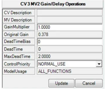
Figure 56: Gain/Delay Operations Popup ... 107

Figure 57: Gain Mapper Function Block in URT Explorer ... 108

Figure 58: Connections to the GM Panel on the Station HMI ... 109

Figure 59: OPC Connection to the Profit Controller’s GM Array... 110

Figure 60: OPC Connection to the Profit Controller’s Gain Delay Changed Data Item ... 110

Figure 61: GM Manipulation Script for PU01 ... 111

Figure 62: UWS Re-configuration with PU05 and PU01 Eliminated ... 112

Figure 63: Gain Delay Matrix for the UWS with PU05 and PU01 Eliminated ... 113

(18)

Figure 65: Range Change Sequence for LT01 Under PI Control (Direct Synthesis Tuning) 118

Figure 66: Range Change Sequence for LT02 Under PI Control (Direct Synthesis Tuning) 119

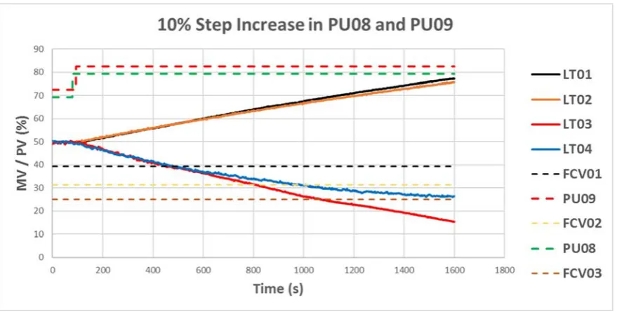
Figure 67: Tank Level Responses to a 10% Step Increase in PU08 and PU09 ... 120

Figure 68: Range Change Sequence for LT01 Under PI Control (Relay Feedback Tuning) 121 Figure 69: Range Change Sequence for LT01 Under Profit Control (Profit Stepper Model) ... 122

Figure 70: Range Change Sequence for LT01 Under Profit Control (Reduced Number of MVs) ... 123

Figure 71: IAE Controller Performance Analysis ... 124

Figure 72: Range Change Sequence for LT01 Under Profit Control (Simulated Model) ... 125

Figure 73: Shewart Control Chart for a Disturbance Introduced under PI Control (Relay Feedback Tuning) ... 127

Figure 74: Shewart Control Chart for a Disturbance Introduced under Profit Control (Profit Stepper Model)... 128

Figure 75: Tank Level Interaction Valves ... 131

Figure 76: Interaction Valve Positioners ... 132

Figure 77: Photograph of the UWS ... 138

Figure 78: PU01 Flowrate Calibration Curve ... 139

(19)

Figure 86: PIS Offline Simulation Input Type Selection... 144

Figure 87: Random Input Sequence for PU0 ... 145

Figure 88: User Prompt to Export the Random Input Step Test Plan to a Data File ... 145

Figure 89: Saving the Random Input Step Test Response to a Data File ... 146

Figure 90: Importing a Data File to the PIS Offline Simulation ... 146

Figure 91: Data File Format for the PIS Offline Simulation ... 146

Figure 92: Simulated Response to Imported Data ... 147

Figure 93: Response Validated by the PIS Offline Simulation ... 148

Figure 94: SSI Offline Simulation MV Selection Menu Box ... 149

Figure 95: Stepping PU01 using the SSI Offline Simulation ... 150

Figure 96: Command Window Snippet from the SSI Offline Simulation ... 151

Figure 97: Changing the Security Level to Manager in PSOS ... 156

Figure 98: Controller Model File In PSOS ... 157

Figure 99: Restarting the Profit Controller in PSOS ... 158

Figure 100: Student Program Read/Write Sub-VIs [30] ... 166

Figure 101: Front Panel of the LabVIEW to Experion Gateway ... 167

Figure 102: UWS Main Display ... 168

Figure 103: UWS Trends Display... 169

Figure 104: Profit Controller Popup ... 170

Figure 105: PID Controller Popup ... 170

Figure 106: Auto Step Popup ... 171

Figure 107: Connection Between the Hydro-electric System and UWS [62] ... 172

Figure 108: Separation of the Hydro-electric System and UWS ... 173

Figure 109: FIT02 Removable Mounting Bracket... 174

(20)

Figure 111:Analysing the Relay Feedback Response ... 178

Figure 112: Set Point Change Sequence under PI Control (Direct Synthesis Tuning) - PV

Response ... 180

Figure 113: Set Point Change Sequence under PI Control (Direct Synthesis Tuning) - MV

Response ... 181

Figure 114: Set Point Change Sequence under PI Control (Relay Feedback Tuning) - PV

Response ... 182

Figure 115: Set Point Change Sequence under PI Control (Relay Feedback Tuning) - MV

Response ... 183

Figure 116: Range Change Sequence under Profit Control (Simulated Model) - PV Response

... 184

Figure 117: Range Change Sequence under Profit Control (Simulated Model) - MV Response

... 185

Figure 118:Range Change Sequence under Profit Control (Profit Stepper Model) - PV

Response ... 186

Figure 119:Range Change Sequence under Profit Control (Profit Stepper Model) - MV

Response ... 187

Figure 120: Range Change Sequence under Profit Control (Reduced Number of MVs) - PV

Response ... 188

Figure 121: Range Change Sequence under Profit Control (Reduced Number of MVs) - MV

(21)

Table

of

Tables

Table 1: Calibration Range for PU01, PU03, PU08 and PU09 ... 46

Table 2: Calibration Range for Different Sized Orifice Diameters for the Outlet of Tank01 . 50 Table 3: Estimated Orifice Plate Calibration Range for the Outlet of Tank03 and Tank04 .... 52

Table 4: Calibration Range for PU05 ... 90

Table 5: Calibration Ranges for the Flow Control Valves ... 95

Table 6: Calibration Range for a 16mm Orifice Diameter ... 98

Table 7: Signal to Noise Ratio Quality Definitions [50] ... 103

Table 8: Gain Mapper Configuration Example ... 107

Table 9: Feedback Controller Parameters - Tuned using the Relay Feedback Test ... 115

Table 10: Feedback Controller Parameters - Tuned using Direct Synthesis ... 115

Table 11: Syntax of the Functions from MATLABs OPC Toolbox ... 153

Table 12:4x4 Model Matrix Developed From Simulated Plant Data ... 159

Table 13:9x5 Model Matrix Developed Using Simulated Plant Data (1/2) ... 160

Table 14:9x5 Model Matrix Developed Using Simulated Plant Data (2/2) ... 161

Table 15:9x5 Model Matrix Developed Using Profit Stepper (1/2) ... 162

Table 16:9x5 Model Matrix Developed Using Profit Stepper (2/2) ... 163

Table 17: Direct Synthesis Feedback Controller Tuning ... 176

(22)

(23)

Table

of

Equations

Equation 1: Stop Watch and Beaker Flowrate Equations ... 44

Equation 2: Temporary Outlet and Verified Pump Flowrate Relationships (Four Tank

Configuration) ... 55

Equation 3:Mass Balance and ODE Surrounding Tank01 ... 56

Equation 4: Discretising an ODE using Euler’s Derivative Approximation [4] ... 57

Equation 5: Updated Tank Outlet Flowrate Relationships (Four Tank Configuration) ... 82

Equation 6: Verified PU05 Flowrate Relationships (Five Tank Configuration) ... 90

Equation 7:Verified Flow Control Valve Flowrate Relationships (Five Tank Configuration)91

Equation 8: Tank 05 Outlet Flowrate Relationship (Five Tank Configuration) ... 94

Equation 9: Verified Outlet Flowrate Relationships for Tank04 (16mm orifice - Five Tank

Configuration) ... 98

Equation 10: Control Chart Limit Calculation [53] ... 126

Equation 11: Direct Synthesis Controller for a Pure Capacity System [4] ... 175

Equation 12: Direct Synthesis Controller for a First Order System [4] ... 175

Equation 13: Calculating the Ultimate Gain from the Relay Feedback Test [4] ... 179

(24)

(25)

Acronyms

and

Abbreviations

APC Advanced Process Control

APD Aspen Plus Dynamics

CEE Control Execution Environment

CGU Control Group Unit

CM Control Module

Co-simulation Cooperative Simulation

COM Component Object Model

cRIO Compact RIO

CV Controlled Variable

DCS Distributed Control System

DMC Dynamic Matrix Control

FCV0# Flow Control Valve 0#

FIT0# Flow Indicator Transmitter 0#

GD Gain Delay

GM Gain Multiplier

HAZOP Hazard and Operability Study

HMI Human Machine Interface

IAE Integral of the Absolute Error ISE Integral of the Square of the Error

L Litre

(26)

m metre

MATLAB Matrix Laboratory

min Minute

mm Millimetre

MPC Model Predictive Control

MV Manipulated Variable

ODE Ordinary Differential Equation

OLE Object Linking and Embedded

OP Operating Point

OPC OLE for Process Control

OTS Operator Training Simulator

PI Proportional and Integral

PID Proportional Integral and Derivative

PIS Predefined Input Sequence

PSES Profit Suite Engineering Studio PSOS Profit Suite Operator Station PSRS Profit Suite Runtime Studio

PU0# Pump 0#

PV Process Variable

RIO Remote Input/Output

RMPCT Robust Model Predictive Control Technology

s Second

(27)

URT Unified Real Time

UWS Universal Water System

VI Virtual Instrument

(28)

‐

Introduction

1.1 Background

Consumer demand is driving the need for increased production rates and lower operating

costs throughout the process industry. As technology advances to meet these demands,

process plants become more complex and operators need to be increasingly upskilled and

specialised. [1] It can take years for them to become entirely familiar with their plant and the

most valuable lessons may only be learned when something goes wrong. It is also a huge loss

when experts retire and valuable knowledge leaves with them. Process simulators have

become a vital tool for anticipating operational problems, capturing potentially lost expertise

and training newcomers. [2] With a virtual replica of the process running in parallel to the

real-world counterpart, undesirable scenarios can be explored in depth and procedures can be

repeated countless times with no damaging ramifications [3].

A review of case studies revealed that process simulations have been successfully used to

tune and commission both conventional feedback and Model Predictive Control (MPC)

systems. However, there were no documented studies surrounding the end-to-end

development of an MPC control system in a simulated environment to be ultimately used on

a real-world system. As MPC relies on a comprehensive process model, the empirical data

requirements are extensive [4]. Consequently, the process must be disturbed by test signals

(29)

1.2 Project Objectives

The objectives of this thesis are as follows:

 To create an offline simulation of a real-world process to supply data for MPC model

identification.

 To adapt the offline simulation to run in real time for the virtual commissioning of an

MPC control system and for operator training.

 To replicate the simulated MPC control system for its real-world counterpart and

assess controller performance.

The proposed approach is to develop a cooperative simulation (co-simulation) between

Matrix Laboratory (MATLAB) and Honeywell’s Advanced Process Control (APC) platform,

Profit Suite. It is hypothesised that, if the process is accurately modelled, a controller

designed using simulated data could be used in the real-world system and Honeywell’s

Robust Model Predictive Control Technology (RMPCT) would handle the model mismatch.

1.3 Report Structure

The following report begins in Chapter 2 with a literature review of relevant case studies. The

formal work of this thesis is separated into two sections. The chapters in each section begin

with a brief introduction followed by a discussion of the methods applied. Section One

(Chapter 3 to Chapter 6) details the development of a co-simulation and MPC control system

for a basic configuration of the Universal Water System (UWS). As a proof of concept, this

section deals primarily with software development. Chapter 3 explains the steps involved

with plant calibration which is used in Chapter 4 to establish a mathematical model. Chapter

5 introduces MPC and outlines the design of a Profit Controller, first for the simulation and

(30)

Section Two (Chapter 7 to Chapter 11) covers the upgrade of the control system and

co-simulation for a more complex configuration of the UWS and explores some advanced Profit

Suite functionality. Chapter 7 highlights the additional plant calibration required to expand

the mathematical model. Chapter 8 introduces Profit Suites step testing platform, Profit

Stepper, for online model identification. Chapter 9 explains how a Profit Controller’s internal

model can be modified dynamically with changing plant conditions. Controller performance

is analysed in Chapter 10 for the controller models identified in the earlier chapters and a

conventional feedback strategy. The report concludes in Chapter 11 with a presentation of the

(31)

‐

Literature

Review

Over the years simulations have become widely used across a number of different industries.

Although literature covers a wide range of applications, this review will focus primarily on

the use of simulations for operator training and control system design within the process

industry. The major themes that appeared throughout the reviewed literature included safety

studies, scenario replication, dynamic real-time operator training platforms, equipment

selection and sizing, offline optimisation and control system design. Issues were highlighted

surrounding the interoperability of software packages from different vendors, as well as the

associated expenses. Solutions to this were presented in various case studies and have been

reviewed accordingly. Although these themes have been studied in a number of contexts, this

chapter will concentrate predominantly on the development of APC solutions – specifically

MPC.

2.1 Simulation use within the Life‐Cycle of a Process Plant

With the increasing complexity of modern process plants, simulations are becoming a vital

tool for use during the design and operational phases of a plant’s life cycle. While it is

important that these plants maintain high production rates at the lowest cost, the primary

objective is for them to operate within safe limits. Many plants run for 24 hours a day, 7 days

a week, and this may continue for years with no downtime. [2] Even though plant operators

may try to maintain operating conditions, they rarely stay constant over time and periodic

optimisation is often required [6]. Bearing in mind the costs associated with a process upset,

operators and engineers cannot simply take an ad hoc approach when making changes.

Furthermore, it is widely accepted that design modifications can be made more easily and

(32)

simulators offer both an effective operator training platform and a means to predict the

outcome of modifications proposed during the design or operational phase. [2]

2.1.1. Plant Safety Design

It is critically important in process plant design that control and safety engineers identify

potentially hazardous events early. A Hazard and Operability Study (HAZOP) is a qualitative

technique used to systematically identify hazardous situations that may arise when a plant

deviates from its intended operation. Root cause analysis can then be applied to each scenario

to identify the initiating event. Finally, a quantitative risk assessment can be carried out to

identify the likelihood and severity of each situation. When a high risk event is identified, to

adhere to safety requirements engineers must alter the design by incorporating Independent

Protection Layers to reduce the risk level. [7]

A case study, presented in [7], investigated the effective use of a distributed dynamic

simulation to aid the safe design of a chemical processing plant. The distributed simulation

comprised a number of smaller sub-processes called Control Group Units (CGU). Each CGU

represented a different stage in a complex hydrodesulphurization chemical process. A

HAZOP was conducted around each CGU and the risk assessment was tightly integrated with

the simulation. Each of the identified hazardous situations was simulated and the results were

used to quantify the associated risk. The simulation was instrumental in identifying fault

propagation between CGUs and, in turn, the entire process. It was also found to significantly

reduce the time required to complete the safety assessment. [7]

(33)

reaction exceeds the rate of heat removal and it can result in fire, thermal degradation,

contamination or even a thermal explosion. A study by [8] investigated a runaway scenario

caused by a cooling system failure on an ethylene oxide plant using an Aspen Plus Dynamic

(APD) process simulation. By repeatedly simulating the scenario it was possible to identify

the early warning signs and devise an appropriate emergency response plan. [8]

2.1.2. Equipment Selection and Sizing

Crosstex and Bryan Research and Engineering [6], made use of a ProMax steady state

simulation to rate the performance of plant equipment and identify potential flaws. The

Gregory Gas Plant Facility, located in Southeast Texas, was the test case for this simulation.

The base process model was built from Process Flow Diagrams and Piping and

Instrumentation Diagrams from the real plant. The simulation was validated by matching the

rating and sizing of all equipment in the model with the real plant and then comparing the

results. It was found to accurately represent the plant’s operation in areas such as product

composition, flowrates, heat duties and horsepower requirements. The physical

characteristics of the various heat exchangers, columns and separators were entered into the

performance rating section of the simulator and the results were compared with those from

the equipment vendors. The simulation was found to be remarkably accurate and the

predicted performance ratings were within +10/-5 % of the vendor ratings. This provided

engineers with the flexibility to assess proposed equipment modifications offline without

disturbing the real process. Further testing presented a number of potential areas for concern,

such as calculated pressure drop through a heat exchanger, actual nozzle size versus

recommended nozzle size, and the approach to flooding within a tower. This information was

(34)

In a study carried out by [9], a phosphoric acid concentration unit was simulated using

Honeywell UniSim Design. The simulation was used to test and compare two different

control configurations in order to identify which would be most effective. It was found that

one of the control strategies was unable to control the evaporator pressure while the other did

so with ease. The simulation was also used to identify frequent mistakes made by process

engineers during operation. It was found that a low level interlock was repeatedly triggered

during the start-up procedure. This resulted in downtime as the pumps needed to be restarted

each time. The simulation was able to test and verify that a low level switch and alarm placed

above the low level interlock switch would help to avoid such situations. Again, this study

allowed engineers to draw conclusions about proposed changes without disturbing the real

process. [9]

2.1.3. Operator Training

During a process plant’s life cycle, decisions and adjustments are traditionally made by

experienced engineers and operators. Unfortunately, when these people retire or change jobs,

their knowledge is not necessarily passed on. [2] This can be detrimental to the efficiency and

safety of the plant. Studies have shown that human error is responsible for 50 % of

production losses in the US process industry and is a factor in 70-90 % of industrial accidents

across most industries. It is accepted that the majority of these human errors are due to

unsatisfactory operator knowledge and the inability to respond appropriately to changing

operating conditions. [9] Simulations can be used as low risk virtual experiments to capture

expert knowledge and use it to train inexperienced engineers and operators [2]. Recent

studies suggest that the most effective way to teach is by combining face-to-face learning

(35)

Simulations have the benefit of being independent of many real-world dynamic constraints.

For example, they can be configured to run much faster than the actual process to decrease

training time. It was found by [10] that, for most simulation work, engineering effectiveness

was maximised when the models could run up to 50 times faster than real time. It was found

that when the simulations ran so slowly that operators could take coffee breaks or start new

tasks while awaiting results, their concentration would lapse. This tended to interrupt the

learning process and significantly reduce efficiency. [10] Alternatively, simulations can be

slowed down to give trainees time to think about how to respond to more challenging

situations. [11]

2.1.4. Predetermined Scenario Handling

The number of operators required in modern control rooms is significantly reduced by the

high levels of automation made available by contemporary technology [12]. It was

highlighted in [1] that the mineral processing industry focuses heavily on developing

technical and hardware solutions. However, there is little effort put into maximising the gains

from emerging technology by training operators effectively. [1] Operators have to deal with

both normal and abnormal situations. Normal operations include factors such as product

quality, emission control, efficiency and profitability while abnormal situationsmight involve

aspects such as speed of recovery, damaged hardware and system failure. [12] It is imperative

that operators are suitably trained to cope with all types of situations. Simulations can be

extended to emulate a wide range of scenarios and provide operators with risk-free training to

prepare for the real-world counterpart. This is particularly relevant for high-risk applications.

[13]

A study presented in [3] used a biodiesel process simulation to investigate scenarios

(36)

bursting disks. The simulation was developed using APD along with the Aspen Operator

Training Simulator (OTS) Framework. The aforementioned scenarios were part of a portfolio

that could be loaded by an instructor at any given time to train new or existing operators. The

operators could then respond to the situations and naturally identify the optimal way to cope.

Repeating the procedure saw the operators become familiar with each situation and

confidently respond with corrective action. This provided them with the necessary skills to

respond when working with the actual process. Furthermore, the OTS could be linked to a

performance evaluation algorithm that would quantifiably verify the most effective way to

respond. [3]

2.1.5. Control System Design

It was suggested in [1] that operator performance can, at times, impose a constraint on control

system performance. Simulations can provide operators with the ability to practise control

system tuning techniques without upsetting the real process. In [3], [14], [15] and [16],

operator training platforms were developed to test different Proportional Integral and

Derivative (PID) controller configurations, parameters, modes and set points. In a simulated

environment, operators have the ability to drive the process unstable with aggressive tuning

without detrimental repercussions. This type of training has been found to build operator

skills and instil confidence prior to entering the control room. [3]

Given its ability to handle multivariable loop interactions and actuator constraints, MPC has

become a preferred strategy in the chemical and petrochemical industries. [17] However, it

was highlighted in [18] that MPC and dynamic operator training simulation software usually

(37)

platform. In [18], blending and distillation process simulations were developed in SimSuite

Pro and connected to the MPC software through a Distributed Control System (DCS). This

enabled operators to experiment with MPC on a high fidelity simulated process, tune the

controllers and examine the connection to the DCS. [18]Both studies were exclusively used

for training purposes and no physical systems were involved.

2.2 Co‐simulation and Connectivity

There is a range of dynamic simulators available in today’s market. Generally, each

simulation platform is best suited to a specific production process. [20] Furthermore, modern

plants tend to have several plant-wide operations which may fall into separate classifications.

Similarly, there are a several MPC software packages to choose from. Despite this, many oil

refining and petrochemical plants will adopt one and use it in a routine way for decades. This

will see plant personnel become proficient with that particular technology but can lead to

complications when companies merge or processes are combined. It can be beneficial to

establish seamless and synchronised communication between different simulation platforms

and MPC systems in order to exploit individual strengths and make use of existing software

licences. This is known as co-simulation. [20]

2.2.1. ActiveX

Object Linking and Embedded (OLE) Automation (later renamed Automation) is a Microsoft

Windows programming application. Automation makes it possible for different applications

to manipulate objects within one another. An Automation server can reveal its functionality

to an Automation client via its Component Object Model (COM) interface. This allows the

client to utilise the services provided by any object exposed by the server. An ActiveX

(38)

Automation client of that control. This client server relationship can be used to transfer data

between software packages from different vendors. [21]

In [22], ActiveX was used to build a co-simulation between APD, MATLAB and Laboratory

Virtual Instrument Engineering (LabVIEW) to develop an MPC strategy for a simulated

distillation process. With an extensive database of chemical properties and applications, APD

is one of the most widely used simulation packages in the chemical industry. However, while

it is useful for analysing dynamic plant behaviour and PID control schemes, it does not

support MPC. The DMCPlus software add-on can be purchased separately from AspenTech

to extend the capabilities of APD. This includes an MPC algorithm known as Dynamic

Matrix Control (DMC). To avoid the additional costs associated with DMCPlus, in [22],

ActiveX servers were developed in MATLAB, LabVIEW and APD to extend the original

APD software functionality. The MPC toolboxes in both LabVIEW and MATLAB were

explored and MPC controller performance was compared to Proportional and Integral (PI).

One of the initial aims was to develop an operator training platform in LabVIEW for students

to experiment with MPC on the simulation in real time. This was not achieved due to a lack

of documentation surrounding the object tree structure and was instead left as a future

recommendation. [22]

2.2.2. OLE for Process Control

One disadvantage of using ActiveX controls is that they are intended to be embedded inside

another application. This means that they are not capable of running standalone. On the other

hand, OLE for Process Control (OPC) Servers can run standalone and are specifically

(39)

from different vendors to communicate seamlessly using a client server approach. An OPC

server can communicate with a device using a vendor specific protocol and then make the

information available to clients via its interface. Once configured, an OPC client can request

the information from the server and use it freely. An application that consumes and supplies

data can be both a client and a server. [24] As of 2009, the OPC market included over 2,500

vendors offering over 15,000 OPC-enabled products. [24]

In [20], a crude oil furnace was co-simulated using two rigorous dynamic simulation

platforms - Apros 6 and NAPCON. Apros 6 can be used for a wide range of processes,

however its primary application areas are power plants (nuclear, combustion and solar) and

pulp and paper mills. NAPCON, on the other hand, has an extensive chemical component

library with built in thermodynamics. To combine their strengths, the two simulators were

interfaced at the heat transfer surface between the coils and crude oil in the furnace. OPC

communication was used for scheduling and data exchange between the two simulation

platforms and a NAPCON MPC controller. [20]

In [25], OPC was used to connect well known simulation and research tools MATLAB and

LabVIEW in a co-simulated environment. This was done to support the study of Advanced

APC and Network Control Systems. The major focus of this study was the development of an

MPC-PID cascaded control system for a simulated non-linear boiler system as seen in Figure

1. The closed loop plant model was deployed as a periodic OPC server on LabVIEW. A

series of step inputs were applied to the system and the data was collected via OPC

connectivity for closed loop model identification. This was achieved using MATLAB’s

Identification Toolbox. Finally, the identified model was used to create the MPC interface in

(40)

simulation environment, Simulink, using functions of the OPC Toolbox. Once tested, it was

connected to the closed loop simulation in LabVIEW. [25]

Figure 1:Co‐simulated MPC‐PI Cascaded Control System. Adapted from [25]

In [19], a real-time vacuum crystalliser process simulation was developed in Simulink.

Variables were passed back and forward between the simulation and a Honeywell Profit

Controller (see section 5.1) using MATLAB’s OPC Read and Write toolboxes, as seen in

Figure 2. The simulation framework was designed as a proof of concept. It was proposed that

a similar setup could be used to test and pre-tune advanced controllers in order to reduce the

amount of onsite time required for commissioning. Further to this, it could be used to train

engineers and operators in the use of APC software. It was suggested that this was the first

(41)

2.3 Summary

There is a wide range of simulation and APC software vendors who understandably

safeguard their products – so interoperability can be a significant hurdle [26]. While some

APC vendors do provide simulation packages that are compatible with their other software,

these generally come with a hefty price tag [27]. However, it is possible to reduce costs by

making use of existing software licenses and bridging the gap between different vendors

using co-simulation [20]. This is an attractive option as it can be challenging to find effective

MPC training tools [18]. OPC has been used in a number of cases to connect simulation and

control applications from different vendors. One particular study presented the first, and what

would appear to be the only, documented integration of Honeywell’s industrially used Profit

Suite software with MATLAB’s simulation environment, Simulink [19]. Other co-simulation

platforms were developed using both OPC and ActiveX controls to study different MPC

software packages [24], [20], [25], [22]. However, while the simulated control systems did

provide some insight into controller development, all of the documented test cases were

based entirely on simulations and there was no real-world result validation.

A major challenge that comes with the implementation of APC is the complexity of the

associated software [5]. A class of APC known as MPC has had notable success with highly

interacting processes as it uses an internal process model to calculate the optimal control

action. [17] Consequently, extensive testing is often required to gather enough data that

sufficiently captures the process dynamics [5]. This not only takes up valuable time but also

means that the process has to be deliberately disturbed for extended periods [5]. Simulations

have been successfully used to train engineers and operators with MPC software prior to

(42)

been done on the use of process simulators to develop the internal model for an MPC

controller to be used on a real process.

(43)

Section

One

Simulation

and

Control

System

Development

Chapter 3 to Chapter 6 in Section One deal with the development of an MPC control system

for the UWS, configured as shown in Figure 3. This section describes the parallel

development of a co-simulated and real-world MPC control system. Chapter 3 discusses plant

calibration and how mathematical estimations can be used to predict unmeasurable process

data. Chapter 4covers the development of offline and real-time process simulations using the

mathematical models developed in the preceding chapter. Chapter 5introduces Profit Suite

and discusses Profit Controller development - first for the real-time simulation and then for

the real-world plant. The open and closed loop simulated responses are analysed in Chapter 6

and the areas of model inaccuracy are highlighted. With the plant under control, the

estimations made in Chapter 3 were refined and the consequential improvements in

simulation fidelity quantified.

(44)

‐

Calibration

Calibration is defined by The Automation, Systems and Instrumentation Dictionary as “a test

during which known values of measurand are applied to the transducer and corresponding

output readings are recorded under specified conditions” [28]. A transducer can measure

variations in a physical quantity but without a known reference point they are meaningless.

An instrument can be calibrated by taking measurements at several points throughout the

calibration range with another instrument of higher accuracy [28]. The calibration range can

be defined as “the region between the limits within which a quantity is measured, received or

transmitted, expressed by stating the lower and upper range values” [28]. The physical

quantities of interest in this study are tank level and volumetric flowrate. The primary

calibration objective of the chapter is to ensure that all level and flow transmitters (LT and

FIT respectively) are outputting the correct values. The secondary objective is to develop a

mathematical model of each flowrate within the system.

3.1 Level Transmitters

All level transmitters (LT) in the plant were calibrated in early 2018 by Murdoch University

engineering students [29]. A guide outlining the calibration procedure is given in [29]. All

four level transmitters (LT01, LT02, LT03 and LT04) were checked by filling each tank from

0% to 100% capacity and confirming that the correct values were output to the instruments

digital display.

3.2 Experimental Flowrate Measurement

The volumetric flowrate of a fluid can be quantified by measuring the volume passing

(45)

measurements, the volumetric flowrate can be calculated as per Equation 1. This technique

will be referred to as the stopwatch and beaker method.

60 ∗ " "

1000 ∗ " "

60000

Equation 1: Stop Watch and Beaker Flowrate Equations

Although this method eliminates the need for costly apparatus, the results are typically

influenced by human error. The largest source of error in this experiment arises from the

measurer’s coordination and reaction time. For the results to be accurate, the beaker must be

moved under the fluid stream precisely as the stopwatch is started and removed exactly as it

is stopped. To reduce such errors, the same individual was employed to take all

measurements during plant calibration, all measurements were repeated and the resulting

flowrates were averaged.

3.3 Pumps with VSD Speed Control

Of the five Variable Speed Drive (VSD)-controlled pumps in the plant, four were required to

control the system in the four-tank configuration (see Figure 3). These include Pump01

(PU01), PU03, PU08 and PU09 - all of which have a flow transmitter installed downstream.

When the plant was commissioned, the pumps were configured to operate between 800 and

1500 RPM as recommended by the manufacturer to avoid low RPM - which can damage the

pump’s electric motor. [30] Consequently, the pumps will only ever run between 53% and

100% of their maximum speed. To calibrate the inline flowmeters, each of the pumps was

(46)

experimental stopwatch and beaker measurements were recorded at each point. The resulting

flowrate data for each pump was plotted against the pump speed percentage for comparison

(see Figure 4).

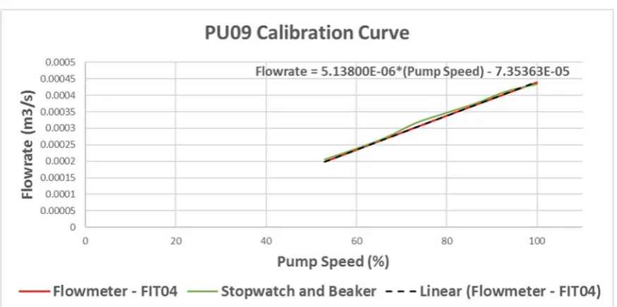
Figure 4: PU09 Flowrate Calibration Curve with Fitted Trend Line

Figure 4 shows that the experimental measurements match closely with the flowmeter

readings. Both sets of data follow the same gradient and the minor positive offset was

considered due to human error. This was the case for all four pumps (see Appendix 2.1) and

it was therefore concluded that the flowmeters were calibrated correctly. Microsoft Excel was

used to fit trend lines to the flowmeter data and ascertain the mathematical relationship

(47)

Table 1: Calibration Range for PU01, PU03, PU08 and PU09 Pump Minimum Flowrate (L/min) Maximum Flowrate (L/min)

PU01 14.88 29.98

PU03 13.97 28.34

PU08 12.16 27.08

PU09 11.89 26.36

3.4 Restriction Orifice Plates

Orifice plates are most frequently used for flow measurement. They are typically constructed

from a machined metal plate containing one or more orificesthrough which fluid will flow.

The plate is clamped between two flanges and mounted in line with a straight section of

piping to create a flow-dependant pressure drop. A differential pressure sensor can be used to

measure the pressure drop and in turn calculate flowrate. Alternatively, a restriction orifice

plate uses the same design principle but aims to maintain a constant pressure loss by

restricting the flowrate. [31]

Initially, the outlet flowrates from each tank were restricted by manually actuated gate valves.

These are not recommended for throttling flow and are rather designed for on/off

applications. If used for flow control, the high velocity fluid impinging against the partially

open disc can cause excessive vibration and damage the seating surfaces. This type of wear

will eventually prevent the valve from shutting off completely. [32] Testing showed that,

with the valves fully open, the inlet flowrates from the pumps could not be raised high

(48)

plates constructed from Polyvinyl Chloride end caps as seen in Figure 5. The gate valves

would then be opened to 100 % and the flow would be throttled by the downstream orifice.

Figure 5: Restriction Orifice Plate

Flowrate through the outlet depends on the surface area of the orifice and the upstream

pressure [31], therefore calibrating the flow through the orifice involved measuring the outlet

flowrate at several tank levels and repeating this for a number of different orifice diameters.

As Tank01 had a downstream flowmeter (FIT07) installed, it was selected as the initial

testing platform. LT01 was maintained at steady state by manually adjusting the speed of

PU01. The flowrate measurements were taken using FIT07 at several steady state tank levels

between 10% and 90%. This was repeated for five different orifice diameters ranging from

(49)

FIT07 gave a reading of 2.7 litre /minute (L/min) during zero flow conditions and the

difference between the reading from FIT01 and FIT07, at each steady state, was also 2.7

L/min. This confirmed a constant offset throughout FIT07’s working range and also indicated

that the variation in the flowrate measurements was consistent with FIT01 - which had been

previously calibrated. In view of this, 2.7 L/min was subtracted from all FIT07 flowrate

readings. A plot of flowrate against tank level, for the range of orifice diameters, can be seen

in Figure 6. As expected, the flowrate increased with orifice diameter as well as tank level.

Figure 6: Plot of LT01 vs Tank01 Outlet Flowrate for Different Restriction Orifice Diameters

The relationship between the tank level and outlet flowrate, for each orifice diameter, was

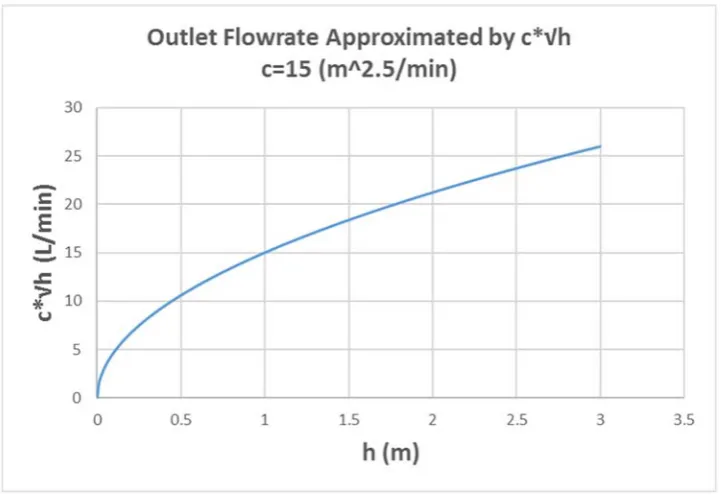
linear. This did not align with the theoretical supposition that the outlet flowrate of a

self-regulatory tank can be approximated by a constant multiplied by the square root of the tank

(50)

Figure 7: Installed Height of Tank01, Tank02, Tank03 and Tank04

As shown in Figure 7, the tanks can only vary by a maximum of 0.87m. However, the

distance between the tank outlet and the orifice plate is 1.68m. It is proposed that the

theorised nonlinearities were negligible due to the head upstream of the orifice only being

able to vary between 1.77m and 2.46m. A plot of the theoretical relationship (see Figure 8)

indicates that as the tank level deviates from 0 m, the relationship becomes increasingly

(51)

Figure 8: Theoretical Relationship between Tank Level and Outflow of a Tank

The calibration range for each orifice diameter, tested on the outlet of Tank01, can be seen in

Table 2.

Table 2: Calibration Range for Different Sized Orifice Diameters for the Outlet of Tank01

Orifice Diameter (mm)

Maximum Flowrate (L/min)

8.1 10.91 13.11

9.9 16.16 19.91

10.5 18.40 22.09

11.5 22.05 30.91

12.9 27.26 33.00

3.4.1. Outlet Flowrate Estimation

It was predicted that the outlet flowrate characteristics for Tank01 and Tank02 would be

(52)

tank bottom were the same in each case (see Figure 7). However for Tank03 and Tank04,

although the tank dimensions were the same, the distance between the tank bottom and

orifice plate was one meter higher. Consequently, the plots shown in Figure 6 were

extrapolated to account for the additional upstream pressure (see Figure 9).

Figure 9: Tank Outlet Flowrate Relationships for Different Sized Orifice Diameters with Extrapolated Trend Lines

By extrapolating the plots, it was assumed that the relationship between tank level and outlet

flowrate would remain linear throughout the extended range. In practice this may not be the

case and it was therefore expected that the mathematical models fitted to the data would hold

some degree of error. The flowrate measurements would be refined at a later stage using the

stopwatch and beaker method once level control had been implemented. This would enable

(53)

models would be sufficiently accurate to simulate the process dynamics at a rudimentary

level.

The estimated calibration range for each orifice diameter attached to Tank03 and Tank04 can

be seen in Table 3.

Table 3: Estimated Orifice Plate Calibration Range for the Outlet of Tank03 and Tank04

Orifice Diameter (mm) Maximum Flowrate (L/min) Maximum Flowrate (L/min)

8.1 15.49 13.29

9.9 20.21 23.96

10.5 22.39 26.09

11.5 31.39 37.24

12.9 33.48 39.22

3.4.2. Orifice Diameter selection

For the plant to be controllable, the outlet flowrate of each tank had to fall within a range

such that the inlet pump would increase the tank level when operating towards its upper limit

and decrease it when operating towards its lower limit. This could be achieved by selecting

the orifice diameter so that its calibration range would fall within the inlet pump’s calibration

range. Orifice plate sizing charts were created by overlaying the pump and orifice diameter

calibration plots, as seen in Figure 10 and Figure 11. Using the charts, a 10.5mm orifice

diameter was selected for Tank01 and Tank02 (see Figure 10) and a 9.9mm diameter was

(54)

Figure 10: Orifice Diameter Selection Chart for Tank01 and Tank02

(55)

‐

Process

Simulation

A process simulation is defined by [33] as the application of mathematics and first principles

(i.e. conservation laws, thermodynamics, transport phenomena and reaction kinetics) to

describe and accurately represent the behaviour of a process. Mathematical models can be

developed to describe either the steady state or dynamic nature of a system. The scope of

each is shown inFigure 12. [33]

Figure 12: Comparison of Steady State and Dynamic Model Scopes. Adapted from [33]

A steady state simulation assumes that all variables are constant with respect to time so, for

the overall mass and energy balances, input will be equal to output and there is no

accumulation within the system. Consequently, a steady state simulation only provides

information about the ultimate state of the process at a particular operating point (i.e. when

all state variables are constant). Conversely, a dynamic simulation takes into account the

accumulation of mass and energy so it is possible to determine the amount of time taken for a

(56)

Simulations can be further classified as either real-time or offline. A discrete-time offline

simulation can be configured to execute with a longer or shorter time-step than the

mathematical model. Offline simulations are typically used to gather data at a faster rate,

whereas real-time simulations are intended to run at the same speed as their physical

counterpart. Real-time simulations are only compatible with a fixed time-step, the duration of

which is vital for effective operation. The time-step must be selected so that the simulator has

time to complete all calculations and then lie idle until the start of the next interval. [34]

4.1 Mathematical Modelling

Flowrate relationships, recovered during plant calibration, are shown in Equation 2. Pump

flowrate equations were verified during calibration and are therefore final. The estimated tank

outlet flowrates, shown in red, would be used temporarily until they were refined and verified

at a later stage.

Verified Pump Flowrate Equations

01 5.02 ∗ 10 01 1.80 ∗ 10

03 5.15 ∗ 10 03 4.17 ∗ 10

08 5.28 ∗ 10 08 7.39 ∗ 10

09 5.14 ∗ 10 09 7.35 ∗ 10

Temporary Tank Outlet Flowrate Equations

01 10.5 6.16 ∗ 10 01 3.07 ∗ 10

02 10.5 6.16 ∗ 10 02 3.07 ∗ 10

(57)

Mass balances were carried out around each tank to develop a system of Ordinary

Differential Equations (ODE) that describe the UWS. The simulation needed to be dynamic

and therefore accumulation within the system had to be considered. The conservation of mass

law stipulates that the rate of mass accumulation within the confines of a system is equal to

the difference between rate of mass entering and leaving the system [4]. As the outlet

flowrate of each tank depends on the tank level, the systems are all classified as

self-regulatory. This means that when a step change is applied to the input, the system will move

to a new steady state rather than increasing or decreasing indefinitely [35]. A mass balance,

and resulting ODE, for a self-regulatory tank level process can be seen Equation 3.

Assuming fluid density remains constant:

Where:

A= Tank Surface Area

5.02 ∗ 10 . 01 1.80 ∗ 10

6.16 ∗ 10 . 100

0.87 3.07 ∗ 10

(58)

Each ODE was discretised so it could be solved iteratively using MATLAB. This was done

using Euler’s derivative approximation (see Equation 4) [4]. The proposed MATLAB script

will store the values from the current time-step and use them to calculate the ODE solution in

the next. Using this technique, the program will be able to update all state variables at each

sampling instance (every ∆ seconds).

∆

∴ ∆ ∆ ∗

And shifted back by ∆ seconds:

∆ ∆ . ∆ ∆

Equation 4: Discretising an ODE using Euler’s Derivative Approximation [4]

4.2 Offline Simulation Development

For the purpose of this project, the offline simulation was designed to rapidly generate

process data. This was achieved by numerically solving the previously introduced

mathematical model in MATLAB. The desired functionality of the program was to enable the

user to specify an input sequence and recover the process response for analysis. Two different

versions of the offline simulation were developed, including the Predefined Input Sequence

(PIS) and the Step by Step Input sequence (SSI).

4.2.1. PIS Offline Simulation

The flow diagram of the PIS offline MATLAB script can be seen in Figure 13. The program

can either generate a random input sequence at discrete points in time or the user can choose

(59)

solve the system of ODEs and, when complete, provides an option to export the results to a

new spreadsheet. If the user chooses to import process data, an option is offered to validate

the simulated response against the imported response on completion. Further details can be

found in Appendix 3.1.

Figure 13: Flow Diagram of the PIS Offline MATLAB Simulation

4.2.2. SSI Offline Simulation

The SSI offline simulation repeatedly prompts the user to select which MV to step, the step

magnitude and step duration. A flow diagram of the MATLAB script is given in Figure 14.

After each step the resulting data plot will update and the user will be prompted to select the

next move. The options include performing another step, erasing a section of data or exiting

the program. The SSI simulation enables dynamic alteration of the input sequence between

(60)

to carry out a precise step test plan while making modifications on the run. When sufficient

data is gathered, the user can opt to end the program and export the results to a spreadsheet.

Further details can be found in Appendix 3.2.

Figure 14: Flow Diagram of the SSI Offline MATLAB Simulation

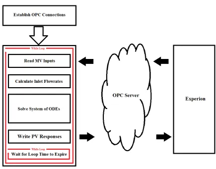
4.3 Real‐time Simulation Development

The real-time simulation was designed to authentically replicate the real-world system in a

virtual environment. This includes the process dynamics and the connection to the DCS. The

objective was to make it feel as realistic as possible so that it could be used as an operator

training tool when later experimenting with MPC. Also, a high fidelity simulation provides a

way to commission a controller in a risk-free environment before transferring it onto the real

plant.

The real-time simulation was built on the foundations of its offline counterpart. However,

rather than running for a finite number of time steps (For Loop), the program continues to run

until it is externally triggered to stop (While Loop). The exit condition on the main loop is

(61)

response speed as desired. The flow diagram of the real-time MATLAB script is given in

Figure 15.

Figure 15: Flow Diagram of the Real‐time MATLAB Simulation

As previously mentioned, to operate in real time, the simulation must be able to complete all

calculations and then lie idle until the start of the next time interval. This was achieved using

MATLAB’s built-in ‘tic’ and ‘toc’ functions. The tic function starts a stopwatch timer and is

called prior to entering the main loop. Once all calculations are complete, the toc function is

called to read the elapsed time from the stopwatch. The program is then forced into a

secondary loop that runs until the toc value reaches the loop time. When this exit condition is

met, the tic function is called again to restart the stopwatch timer. A timestamp is read from

(62)

A number of functions from MALAB’s OPC Toolbox were used to establish a seamless

connection to the OPC server. The functions required to build the real-time simulation are

defined in Appendix 4.

4.3.1. Honeywell Experion Configuration

Experion is Honeywell’s control and safety system that was designed to expand the role of

distributed control and provide seamless plant-wide connectivity [36]. At Murdoch

University, the Experion2 server is host to an instantiation of Experion that can be used by

students to experiment with the software. A guide to the configuration of Experion and its

associated applications can be found in [37]. The following definitions clarify the

Experion-specific terminology used in the following chapter:

 Asset: An asset is defined by Honeywell as a database entity that represents a

particular item within an enterprise. Assets are named such that engineers and

operators can easily isolate and identify plant equipment without having to remember

a vast array of obscure tag names. [37]

 Simulated C300 Controller (SIMC300): Not to be confused with the process

simulation, a SIMC300 controller is a virtual process controller used to execute

control functions through Control Modules (CM) in the Control Execution

Environment (CEE). [38]

 CM: A CM is simply a container for its respective function blocks which can be soft

wired together to deliver their specific function. A PID controller is an example of a

(63)

Figure 16: Control Modules Executed by the UWS_Simulation SIMC300 Controller

A single CM was created for each area of the plant and all were assigned to the UWS_SIM

parent asset. Every MV within the CM was connected to the Operating Point (OP) output of a

PID controller, as seen in Figure 17. In manual mode the controller writes the OP input

directly to the output whereas in automatic mode it reads the set point and calculates the OP

output using a PID algorithm. Numeric function blocks were created to hold pump,

flowmeter and tank level readings while digital values such as pump and solenoid states were

held using boolean flags.

Parallel Development of a Real-time Co-Simulation and MPC Control System for the Universal Water System