Development of a low cost robot system for autonomous measuring of spatial ﬁeld distributions

(1)

Adv. Radio Sci., 10, 1–5, 2012 www.adv-radio-sci.net/10/1/2012/ doi:10.5194/ars-10-1-2012

Advances in

Radio Science

Development of a low cost robot system for autonomous measuring

of spatial field distributions

B. Schetelig1_{, S. Parr}1_{, S. Potthast}2_{, and S. Dickmann}1

1_{Faculty of Electrical Engineering, Helmut-Schmidt-University/University of the Federal Armed Forces Hamburg, Germany} 2_{Bundeswehr Research Institute for Protective Technologies and NBC Protection (WIS) Munster, Germany}

Correspondence to: B. Schetelig ([email protected])

Abstract. A new kind of a modular multi-purpose robot sys-tem is developed to measure the spatial field distributions of very large as well as of small and crowded areas. The probe is automatically placed at a number of pre-defined positions where measurements are carried out. The advantages of this system are its very low influence on the measured field as well as its wide area of possible applications. In addition, the initial costs are quite low. In this paper the theory underly-ing the measurement principle is explained. The accuracy is analyzed and sample measurements are presented.

1 Introduction

In the context of electromagnetic compatibility, the knowl-edge of the electromagnetic field distribution in a certain plane or volume is often required. This information can be used to verify the efficiency of shielding measures or to calibrate field simulators, for example. During such mea-surement campaigns, usually a large amount of data is col-lected for a lot of positions in the test area. Taking these measurements manually can be very time-consuming. To speed-up the process, the field probe can be placed at the designated positions by a robot. There are several special-ized automated measurement systems, designed for special applications (e.g. Haake, 2010). Most of these systems cover a given maximum volume depending on its skeleton size. The probe manipulation is usually done with rectangularly arranged wooden or plastic arms.

The disadvantage of these systems is that due to their fixed-size arms and skeleton they are limited to applications matching their size. If the volume under test is too small, the robot cannot be placed inside. If it is much larger than the scanning area of the robot, the total measurement has to be divided into several parts. In addition, such systems often are too big to speak of an easily movable measuring device.

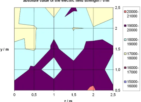
To overcome these disadvantages, the system presented in this paper uses a different approach. To achieve mobility and to cover measurement sites of very different sizes, the mea-surement probe is positioned at the meamea-surement points us-ing two belts (Fig. 1). By manipulatus-ing the lengths of these two belts, it is possible to move the probe to any requested position. By using belts with adequate lengths, it is possible to vary the size of the covered area very easily. In spite of this variability, the total system mainly consists of two actu-ator boxes and two belts. In the presented setup, rubber belts are used which are armed with fibreglass to ensure both ten-sile strength and a very small influence of the measurement system on the field to be measured.

2 Theory

The field probe is placed at the requested position(xm,ym) in the measurement plane by pulling and releasing the belts. The necessary lengths of the belts for a placement can be calculated by

li= q

(xm−xi)2+(ym−yi)2, (1)

with: li: length of the uncoiled parts of the belts, (xi,yi): positions of the actuator boxes.

To enhance the precision, one has to take into account that the belts are not ideal strings. The belts get stretched a little bit when attaching heavy sensors. This influence can usually be ignored if using belts that are oversized with re-spect to the expected loads. Another influence comes from the weight of the belts itself. The belts do not connect their fixing points in straight ways but are sagging the more the sensor weight is getting smaller in relation to the weight of the belts. From the balance of forces at every positionx of

(2)

2 B. Schetelig et al.: A low cost robot system for autonomous measuring of spatial field distributions Manuscript prepared for J. Name

with version 3.2 of the LA_{TEX class copernicus.cls.} Date: 20 March 2012

Development of a low cost robot system for autonomous measuring

of spatial field distributions

B. Schetelig1_{, S. Parr}1_{, S. Potthast}2_{, and S. Dickmann}1

1_{Faculty of Electrical Engineering, Helmut-Schmidt-University / University of the Federal Armed Forces Hamburg, Germany} 2_{Bundeswehr Research Institute for Protective Technologies and NBC Protection (WIS) Munster, Germany}

Abstract.A new kind of a modular multi-purpose robot sys-tem is developed to measure the spatial field distributions of very large as well as of small and crowded areas. The probe is automatically placed at a number of pre-defined positions where measurements are carried out. The advantages of this system are its very low influence on the measured field as well as its wide area of possible applications. In addition, the initial costs are quite low. In this paper the theory underlying the measurement principle is explained. The accuracy is an-alyzed and sample measurements are presented.

1 Introduction

In the context of electromagnetic compatibility, the knowl-edge of the electromagnetic field distribution in a certain plane or volume is often required. This information can be used to verify the efficiency of shielding measures or to cal-ibrate field simulators, for example. During such measure-ment campaigns, usually a large amount of data is collected for a lot of positions in the test area. Taking these measure-ments manually can be very time-consuming. To speed-up the process, the field probe can be placed at the designated positions by a robot. There are several specialized auto-mated measurement systems, designed for special applica-tions (e.g. (Haake, 2010)). Most of these systems cover a given maximum volume depending on its skeleton size. The probe manipulation is usually done with rectangularly arranged wooden or plastic arms.

The disadvantage of these systems is that due to their fixed-size arms and skeleton they are limited to applications matching their size. If the volume under test is too small, the robot cannot be placed inside. If it is much larger than the scanning area of the robot, the total measurement has to be

Correspondence to:B. Schetelig [email protected]

m·g·dl

φ2(x+dx)

(x1,y1) (x2,y2)

actuators

probe

(xm,ym)

F2(x) F2(x+dx)

dl belt 2 y x belt 1 dy dx

Fig. 1.Positioning a measurement probe in an electromagnetic field using belts

divided into several parts. In addition, such systems often are too big to speak of an easily movable measuring device.

To overcome these disadvantages, the system presented in this paper uses a different approach. To achieve mobility and to cover measurement sites of very different sizes, the mea-surement probe is positioned at the meamea-surement points us-ing two belts (Fig. 1). By manipulatus-ing the lengths of these two belts, it is possible to move the probe to any requested position. By using belts with adequate lengths, it is possible to vary the size of the covered area very easily. In spite of this variability, the total system mainly consists of two actu-ator boxes and two belts. In the presented setup, rubber belts are used which are armed with fibreglass to ensure both ten-sile strength and a very small influence of the measurement system on the field to be measured.

2 Theory

The field probe is placed at the requested position(xm,ym) in the measurement plane by pulling and releasing the belts. The necessary lengths of the belts for a placement can be Fig. 1. Positioning a measurement probe in an electromagnetic field

using belts.

each belt (Fig. 1), a non-linear secondary order differential equation can be derived (Hagedorn, 2006):

d2y dx2=

m·g Fx · s 1+ _d_y dx 2 , (2)

with:m: weight of the belts per element dl,g: gravity accel-eration.Fx=F·cos(φ)is the horizontal force at each belt.

The solution of this differential equation is the so-called catenary equation:

y(x,x0,y0,k)= 1

kcosh(k(x−x0))− 1

k+y0, (3)

with:(x0,y0): shift of the catenary and: k:=m·g

Fx

. (4)

Equation (3) must be applied separately to the left and the right belt, as they usually have different shapes (Fig. 1). The balance of forces at the positions of the actuators (x1,y1), (x2,y2)and of the probe (xm,ym)allow to derive a set of equations which can be used to calculate the shift-parameters x0,y0for both belts (x10,y10,x20,y20).

The requested lengths of both belts can be calculated as

l1,2= ± Z xm

x1,2

dl= ± Z xm

x1,2 s 1+ _d_y dx 2 dx = ± Z xm

x1,2

1 k

d2y

dx2 dx= ± 1 k· dy dx xm x1,2 , (5)

whereas the derivation of Eq. (3) is used: l1=

sinh(k·(xm−x10))−sinh(k·(x1−x10))

k ,

l2=

sinh(k·(x2−x20))−sinh(k·(xm−x20))

k . (6)

The quantitykcan be calculated according to Eq. (4). As the horizontal forceFxis not exactly known a priori, a first estimation value has to be calculated assuming that the per

2 Schetelig et al.: Development of a low cost robot system for autonomous measuring of spatial field distributions

Fig. 2. Measurement setup in the DIES EMP simulator Munster. The actuators are mounted on a mobile wooden frame.

calculated by

li= p

(xm−xi)2+ (ym−yi)2, (1)

with: li: length of the uncoiled parts of the belts, (xi,yi): positions of the actuator boxes.

To enhance the precision, one has to take into account that the belts are not ideal strings. The belts get stretched a little bit when attaching heavy sensors. This influence can usually be ignored if using belts that are oversized with respect to the expected loads. Another influence comes from the weight of the belts itself. The belts do not connect their fixing points in straight ways but are sagging the more the sensor weight is getting smaller in relation to the weight of the belts. From the balance of forces at every positionxof each belt (Fig. 1), a non-linear secondary order differential equation can be derived (Hagedorn, 2006):

d2y dx2=

m·g Fx · s 1 + dy dx 2 , (2)

with:m: weight of the belts per elementdl,g: gravity accel-eration.Fx=F·cos(φ)is the horizontal force at each belt.

The solution of this differential equation is the so-called catenary equation:

y(x,x0,y0,k) =

1

kcosh(k(x−x0))− 1

k+y0, (3)

with:(x0,y0): shift of the catenary and:

k:=m·g Fx

. (4)

Eq. 3 must be applied separately to the left and the right belt, as they usually have different shapes (Fig. 1). The

balance of forces at the positions of the actuators(x1,y1),

(x2,y2)and of the probe (xm,ym)allow to derive a set of

equations which can be used to calculate the shift-parameters x0,y0for both belts (x10,y10,x20,y20).

The requested lengths of both belts can be calculated as

l1,2=±

Z xm

x1,2

dl=± Z xm

x1,2

s 1 + dy dx 2 dx =± Z xm

x1,2

1 k

d2y

dx2 dx=±

1 k· dy dx xm

x1,2

, (5)

whereas the derivation of eq. 3 is used:

l1=

sinh(k·(xm−x10))−sinh(k·(x1−x10))

k , (6)

l2=

sinh(k·(x2−x20))−sinh(k·(xm−x20))

k . (7)

The quantitykcan be calculated according to eq. 4. As the horizontal forceFxis not exactly known a priori, a first

estimation value has to be calculated assuming that the per unit weight of the belts is zero. In this borderline case,Fx

can be calculated from the geometry as:

Fx=

cos(φ1)·cos(φ2)

sin(φ2−φ1)

·M·g , (8)

with: M: weight of the sensor and φ1,2: angles between

horizon and the belts.

The final value ofkis determined by an iterative approach by:

knew= [sinh(k·(xm−x20))−sinh(k·(xm−x10))]·

m M .

(9)

The precision of placing the probe depends on its absolute position in the scanning area. Horizontally in the middle be-tween the actuators at the bottom of the scanning area, the positioning precision is the highest with a given pulling pre-cision of the stepping motor. Moving the probe up towards its highest possible position, the accuracy is decreasing. The same way, the forceFi to be applied on the belts is getting larger and larger. It can be derived as

F1,2=

M·g·cos(φ2,1)

cos(φ1)·sin(φ2)−sin(φ1)·cos(φ2)

, (10)

if the weight of the belts is neglected for simplification.

3 Applied Mechanics

Previous work (Haake and ter Haseborg, 2008) has shown that the type of rope or belt chosen is critical for the precision of the system. A rope is not adequate for precise positioning. The main problem is that it is not possible to measure the Fig. 2. Measurement setup in the DIES EMP simulator Munster.

The actuators are mounted on a mobile wooden frame.

unit weight of the belts is zero. In this borderline case,Fx can be calculated from the geometry as:

Fx=

cos(φ1)·cos(φ2) sin(φ2−φ1)

·M·g , (7)

with: M: weight of the sensor and φ1,2: angles between horizon and the belts.

The final value of k is determined by an iterative approach by:

knew=[sinh(k·(xm−x20))−sinh(k·(xm−x10))]· m M . (8) The precision of placing the probe depends on its absolute position in the scanning area. Horizontally in the middle be-tween the actuators at the bottom of the scanning area, the positioning precision is the highest with a given pulling pre-cision of the stepping motor. Moving the probe up towards its highest possible position, the accuracy is decreasing. The same way, the forceFi to be applied on the belts is getting larger and larger. It can be derived as

F1,2=

M·g·cos(φ2,1)

cos(φ1)·sin(φ2)−sin(φ1)·cos(φ2)

, (9)

if the weight of the belts is neglected for simplification.

3 Applied mechanics

Previous work (Haake and ter Haseborg, 2008) has shown that the type of rope or belt chosen is critical for the precision of the system. A rope is not adequate for precise positioning. The main problem is that it is not possible to measure the length of the uncoiled rope in a sufficient precise and reliable way. One reason is that the rope is always slipping a bit at the cylinder, which is counting the length of the uncoiled rope. In addition, even high-performance Dyneema ropes stretch too

(3)

B. Schetelig et al.: A low cost robot system for autonomous measuring of spatial field distributionsSchetelig et al.: Development of a low cost robot system for autonomous measuring of spatial field distributions 33

Fig. 3.CAD drawing of one of the actuator boxes

length of the uncoiled rope in a sufficient precise and reliable way. One reason is that the rope is always slipping a bit at the cylinder, which is counting the length of the uncoiled rope. In addition, even high-performance Dyneema ropes stretch too much, depending on the position of the sensor, its weight and even the actual kind of coiling operation: The rope usually runs over some deflection rollers. In this area, the lengthen-ing of the rope depends on whether the motor winds the rope up (more stretching) or unwinds it (less stretching).

These difficulties can be overcome by using a cam belt. It cannot slip and in combination with a toothed wheel it is perfect for a precise calculation of the actual length. In ad-dition, there are several fibreglass-armed cam belts available that have almost no lengthening when loaded with the sensor weight.

The mechanical setup is simplified, too. Stepping motors have a fourth state (besides “off”, “right”, “left”): It can act as a brake and fix the sensor at the desired positions. So, no additional elements are needed. In Fig. 3, the inside of one of the actuator boxes is presented. The belt can be seen on the left, moved by the motor on the inside. Below, you find the PCB controlling the motor. It consists of a power electronics area and a section realizing the communication with the personal computer, which controls the measurement devices. Data enters the box via a full duplex optical data link. The small box on the upper right is the appropriate

converter.

The entire system is designed to work with a drag force Fiof up to44Nat each cam belt. The maximum weight of the sensor depends on this limit and the size of the respec-tive measurement area. The conveying velocity of the belt is 21,4mm_s .

4 Control electronics and software

In each of the actuator boxes, identical PCBs can be found. They are equipped with Atmel ATMega32 microcontrollers for communication with the personal computer and to con-trol the power electronics sections. This section of the PCB mainly consists of the STMicroelectronics devices L297, L298N and the belonging external circuit elements. These devices are used to easily drive the stepping motor using the microcontroller. The microcontrollers communicate with the personal computer via a full duplex RS-485 interface (MAX488, MAX489). This kind of bus system was chosen as its differential wires help to withstand the influence of ex-ternal electromagnetic field. The bus cables are connected to a PC interface which translates the RS-485 signals to USB. The interface is detected by the computer as a virtual COM port.

To reduce the vulnerability even more, the RS-485 copper wires connecting the actuator boxes with the interface can be replaced by fibre optical wires. Additional converters in the boxes and the interface execute a code-transparent transla-tion.

To ensure the electromagnetic compatibility, the electron-ics and the motor are encapsulated in a metal box that is sealed by a tight row of screws. All feed-throughs are manu-factured very carefully. The data connection is realized with a fibre optical link. Power supply uses shielded cables and connectors. In addition, filters are applied at the ports of the PCB and the power supply. These measures allow operation up to an electric field strength of at least32 kV

m.

The entire system is controlled by a Matlab-based com-puter programme. Nevertheless, the open documentation of all available instructions, which can be sent to the actuator box microcontrollers, allow to connect the hardware to any other programming environment that is able to communicate via a serial computer port.

5 Precision of positioning

The precision of sensor positioning depends on the accuracy of the rotational movement of the motor and the modelling accuracy of the belt catenaries. It is also quite important to set up the measurement site properly. That means that the positioning can only work sufficient, if the vertical and hor-izontal distances between the actuator boxes are known ex-actly and this data is fed into the control software.

Fig. 3. CAD drawing of one of the actuator boxes.

Fig. 4.Positioning deviations in the horizontal direction

Fig. 5.Positioning deviations in the vertical direction

In the presented setup, a step of the motor equals 0.45 de-grees at the gear shaft. One degree at the shaft results in a belt drive of0.2mm. This allows to coil up and uncoil the belt very precisely. From this follows that the positioning faults mainly result from a poor measurement of the distance between the boxes and inaccurate modelling of the shape of the belts.

In Fig. 4 and Fig. 5 the positioning accuracy is measured in a typical measurement setup for horizontal as well as verti-cal movement. The boxes were mounted on a wooden frame

Fig. 6. Measurement setups in the EMP simulator. Left pictures: transversal measurement, right pictures: length-wise measurement

horizontal precision is best in the middle between the boxes and decreases quite symmetrically towards the left and the right end. To enhance the area of high precision in the mid-dle, the distance between the mounting positions of the boxes can be increased. The deviations in the vertical direction are limited to6mmin this setup.

The precision of positioning of the field probe is sufficient for the intended use of measuring the spatial field distribution of an EMP simulator.

6 Field measurements in the EMP simulator

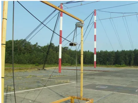
Test measurements were carried out at the DIES sim-ulator (“Deutsches Impulserzeugendes System zur EMP-Simulation”) in Munster in two measurement planes. Their orientations are sketched in Fig. 6. The electromagnetic pulse is generated at the left end (side view) with a Marx generator and propagates along the expanding transmission line. At the right end, the line ends in a termination network.

Fig. 7 shows the spatial distribution of the electric field with a maximum field strength of20 kV_m in the transversal plane. The larger field strength in the lower area can be traced back to the fact that only the vertical component is measured by the sensor. In the upper area, the field lines are slightly bent and are not longer totally vertical as they have to be rectangular to the septum.

The length-wise measurement plane is shown in Fig. 8. The generator is placed at the left end. As expected, the field strength decreases with growing x-values. This can be ex-plained with the increasing distance between generator and Fig. 4. Positioning deviations in the horizontal direction.

much, depending on the position of the sensor, its weight and even the actual kind of coiling operation: The rope usually runs over some deflection rollers. In this area, the lengthen-ing of the rope depends on whether the motor winds the rope up (more stretching) or unwinds it (less stretching).

In the presented setup, a step of the motor equals 0.45 de-grees at the gear shaft. One degree at the shaft results in a

belt drive of0.2mm. This allows to coil up and uncoil the

belt very precisely. From this follows that the positioning faults mainly result from a poor measurement of the distance between the boxes and inaccurate modelling of the shape of the belts.

(cf. Fig. 2). The deviations are measured in a range of2.4m

(horizontally) and1.95m(vertically). Fig. 4 shows that the

horizontal precision is best in the middle between the boxes and decreases quite symmetrically towards the left and the right end. To enhance the area of high precision in the mid-dle, the distance between the mounting positions of the boxes can be increased. The deviations in the vertical direction are

limited to6mmin this setup.

Fig. 7 shows the spatial distribution of the electric field

with a maximum field strength of 20 kV_m in the transversal

plane. The larger field strength in the lower area can be traced back to the fact that only the vertical component is measured by the sensor. In the upper area, the field lines are slightly bent and are not longer totally vertical as they have to be rectangular to the septum.

The length-wise measurement plane is shown in Fig. 8. The generator is placed at the left end. As expected, the field strength decreases with growing x-values. This can be ex-plained with the increasing distance between generator and measurement point and with the growing distance between floor and septum.

Fig. 5. Positioning deviations in the vertical direction.

In the presented setup, a step of the motor equals 0.45 de-grees at the gear shaft. One degree at the shaft results in a

belt drive of0.2mm. This allows to coil up and uncoil the

belt very precisely. From this follows that the positioning faults mainly result from a poor measurement of the distance between the boxes and inaccurate modelling of the shape of the belts.

(cf. Fig. 2). The deviations are measured in a range of2.4m

(horizontally) and1.95m(vertically). Fig. 4 shows that the

horizontal precision is best in the middle between the boxes and decreases quite symmetrically towards the left and the right end. To enhance the area of high precision in the mid-dle, the distance between the mounting positions of the boxes can be increased. The deviations in the vertical direction are

limited to6mmin this setup.

Fig. 7 shows the spatial distribution of the electric field

with a maximum field strength of20 kV_m in the transversal

plane. The larger field strength in the lower area can be traced back to the fact that only the vertical component is measured by the sensor. In the upper area, the field lines are slightly bent and are not longer totally vertical as they have to be rectangular to the septum.

The length-wise measurement plane is shown in Fig. 8. The generator is placed at the left end. As expected, the field strength decreases with growing x-values. This can be ex-plained with the increasing distance between generator and measurement point and with the growing distance between floor and septum.

Fig. 6. Measurement setups in the EMP simulator. Left pic-tures: transversal measurement, right picpic-tures: length-wise mea-surement.

These difficulties can be overcome by using a cam belt. It cannot slip and in combination with a toothed wheel it is perfect for a precise calculation of the actual length. In addition, there are several fibreglass-armed cam belts avail-able that have almost no lengthening when loaded with the sensor weight.

The mechanical setup is simplified, too. Stepping motors have a fourth state (besides “off”, “right”, “left”): it can act as a brake and fix the sensor at the desired positions. So, no additional elements are needed. In Fig. 3, the inside of one of the actuator boxes is presented. The belt can be seen on the left, moved by the motor on the inside. Below, you find the PCB controlling the motor. It consists of a power electron-ics area and a section realizing the communication with the personal computer, which controls the measurement devices.

(4)

4 B. Schetelig et al.: A low cost robot system for autonomous measuring of spatial field distributions

Schetelig et al.: Development of a low cost robot system for autonomous measuring of spatial field distributions 5

Fig. 7. Vertical component of the spatial field distribution in the DIES EMP simulator (transversal plane)

Fig. 8. Vertical component of the spatial field distribution in the DIES EMP simulator (length-wise plane)

7 Conclusions

In this paper we presented a multi-purpose robot system for autonomous field measurements. Its concept allows the ap-plication in very large as well as in very narrow and crowded environments. Due to its modularity, it can be easily moved to other test sites. To minimize the distortion of the measured field caused by the system, fibreglass-armed belts are used to position the sensor. Summarized, it is a very easy to handle, reliable and yet economic system.

References

Haake, K.: Automatisierte Messsysteme für elektromagnetische Felder komplexer Strahlungsquellen, Ph.D. thesis, Technische Universität Hamburg-Harburg, 2010.

Haake, K. and ter Haseborg, J. L.: Development of a modular low cost robot for scanning the electromagnetic field within very

large arbitrary areas or volumes, Serbian Journal of Electrical Engineering, 5, 49–56, 2008.

Hagedorn, P.: Technische Mechanik, Band 1 - Statik, Harri Deutsch Verlag, 2006.

Fig. 7. Vertical component of the spatial field distribution in the

DIES EMP simulator (transversal plane).

Data enters the box via a full duplex optical data link. The small box on the upper right is the appropriate converter.

The entire system is designed to work with a drag force Fi of up to 44 N at each cam belt. The maximum weight of the sensor depends on this limit and the size of the respec-tive measurement area. The conveying velocity of the belt is 21.4 mm s−1.

4 Control electronics and software

In each of the actuator boxes, identical PCBs can be found. They are equipped with Atmel ATMega32 microcontrollers for communication with the personal computer and to con-trol the power electronics sections. This section of the PCB mainly consists of the STMicroelectronics devices L297, L298N and the belonging external circuit elements. These devices are used to easily drive the stepping motor using the microcontroller. The microcontrollers communicate with the personal computer via a full duplex RS-485 interface (MAX488, MAX489). This kind of bus system was cho-sen as its differential wires help to withstand the influence of external electromagnetic field. The bus cables are con-nected to a PC interface which translates the RS-485 signals to USB. The interface is detected by the computer as a virtual COM port.

To reduce the vulnerability even more, the RS-485 cop-per wires connecting the actuator boxes with the interface can be replaced by fibre optical wires. Additional convert-ers in the boxes and the interface execute a code-transparent translation.

To ensure the electromagnetic compatibility, the electron-ics and the motor are encapsulated in a metal box that is sealed by a tight row of screws. All feed-throughs are manu-factured very carefully. The data connection is realized with a fibre optical link. Power supply uses shielded cables and

Schetelig et al.: Development of a low cost robot system for autonomous measuring of spatial field distributions 5

Fig. 7. Vertical component of the spatial field distribution in the DIES EMP simulator (transversal plane)

Fig. 8. Vertical component of the spatial field distribution in the DIES EMP simulator (length-wise plane)

7 Conclusions

References

Haake, K.: Automatisierte Messsysteme für elektromagnetische Felder komplexer Strahlungsquellen, Ph.D. thesis, Technische Universität Hamburg-Harburg, 2010.

Haake, K. and ter Haseborg, J. L.: Development of a modular low cost robot for scanning the electromagnetic field within very

large arbitrary areas or volumes, Serbian Journal of Electrical Engineering, 5, 49–56, 2008.

Hagedorn, P.: Technische Mechanik, Band 1 - Statik, Harri Deutsch Verlag, 2006.

Fig. 8. Vertical component of the spatial field distribution in the

DIES EMP simulator (length-wise plane).

connectors. In addition, filters are applied at the ports of the PCB and the power supply. These measures allow operation up to an electric field strength of at least 32 kV m−1.

The entire system is controlled by a Matlab-based com-puter programme. Nevertheless, the open documentation of all available instructions, which can be sent to the actuator box microcontrollers, allow to connect the hardware to any other programming environment that is able to communicate via a serial computer port.

5 Precision of positioning

The precision of sensor positioning depends on the accuracy of the rotational movement of the motor and the modelling accuracy of the belt catenaries. It is also quite important to set up the measurement site properly. That means that the positioning can only work sufficient, if the vertical and horizontal distances between the actuator boxes are known exactly and this data is fed into the control software.

In the presented setup, a step of the motor equals 0.45 de-grees at the gear shaft. One degree at the shaft results in a belt drive of 0.2 mm. This allows to coil up and uncoil the belt very precisely. From this follows that the positioning faults mainly result from a poor measurement of the distance between the boxes and inaccurate modelling of the shape of the belts.

In Figs. 4 and 5 the positioning accuracy is measured in a typical measurement setup for horizontal as well as ver-tical movement. The boxes were mounted on a wooden frame (cf. Fig. 2). The deviations are measured in a range of 2.4 m (horizontally) and 1.95 m (vertically). Figure 4 shows that the horizontal precision is best in the middle between the boxes and decreases quite symmetrically towards the left and the right end. To enhance the area of high precision in the middle, the distance between the mounting positions of the boxes can be increased. The deviations in the vertical direction are limited to 6 mm in this setup.

(5)

B. Schetelig et al.: A low cost robot system for autonomous measuring of spatial field distributions 5

6 Field measurements in the EMP simulator

Test measurements were carried out at the DIES sim-ulator (“Deutsches Impulserzeugendes System zur EMP-Simulation”) in Munster in two measurement planes. Their orientations are sketched in Fig. 6. The electromagnetic pulse is generated at the left end (side view) with a Marx generator and propagates along the expanding transmission line. At the right end, the line ends in a termination network. Figure 7 shows the spatial distribution of the electric field with a maximum field strength of 20 kV m−1in the transver-sal plane. The larger field strength in the lower area can be traced back to the fact that only the vertical component is measured by the sensor. In the upper area, the field lines are slightly bent and are not longer totally vertical as they have to be rectangular to the septum.

The length-wise measurement plane is shown in Fig. 8. The generator is placed at the left end. As expected, the field strength decreases with growingx-values. This can be ex-plained with the increasing distance between generator and measurement point and with the growing distance between floor and septum.

7 Conclusions

References

Haake, K.: Automatisierte Messsysteme f¨ur elektromagnetische Felder komplexer Strahlungsquellen, Ph.D. Thesis, Technische Universit¨at Hamburg-Harburg, 2010.

Haake, K. and ter Haseborg, J. L.: Development of a modular low cost robot for scanning the electromagnetic field within very large arbitrary areas or volumes, Serbian Journal of Electrical Engineering, 5, 49–56, 2008.

Hagedorn, P.: Technische Mechanik, Band 1 – Statik, Harri Deutsch Verlag, 2006.