Biomimetic spectro-temporal features for music instrument recognition in isolated notes and solo phrases

R E S E A R C H

Open Access

Biomimetic spectro-temporal features for

music instrument recognition in isolated notes

and solo phrases

Kailash Patil and Mounya Elhilali

Abstract

The identity of musical instruments is reflected in the acoustic attributes of musical notes played with them. Recently, it has been argued that these characteristics of musical identity (or timbre) can be best captured through an analysis that encompasses both time and frequency domains; with a focus on the modulations or changes in the signal in the spectrotemporal space. This representation mimics the spectrotemporal receptive field (STRF) analysis believed to underlie processing in the central mammalian auditory system, particularly at the level of primary auditory cortex. How well does this STRF representation capture timbral identity of musical instruments in continuous solo recordings remains unclear. The current work investigates the applicability of the STRF feature space for instrument recognition in solo musical phrases and explores best approaches to leveraging knowledge from isolated musical notes for instrument recognition in solo recordings. The study presents an approach for parsing solo performances into their individual note constituents and adapting back-end classifiers using support vector machines to achieve a generalization of instrument recognition to off-the-shelf, commercially available solo music.

1 Introduction

Research into the nature of musical timbre often focuses on the role of physical attributes of each musical instru-ment and how it colors the sound produced to give it its unique identity. The literature often enumerates spec-tral and temporal identifiers of musical timbre. Specspec-tral information is historically the most studied dimension for musical instrument identification. It spans the magnitude spectrum envelope or relative amplitude of harmonic par-tials [1–3], number of harmonics [4], spectral centroid [5–7], spectral energy distribution [7, 8] and spectral irregularity [9]. Temporal characteristics of musical notes are equally important in shaping sound identity; includ-ing onset information [10], temporal envelope profile [11], energy buildup or attack over time [3, 12], vibrato [13, 14] as well as spectral flux over time [9]. Indeed, most studies have converged on the fact that ajoinedspace of spectral and temporal information is necessary to fully describe the space of musical timbre and capture the phys-ical attributes that are perceptually relevant for describing

*Correspondence: [email protected]

Department of Electrical and Computer Engineering, Center for Speech and Language Processing, Johns Hopkins University, Baltimore, MD, USA

each musical instrument. Research based on perceptual judgments of natural or manipulated notes as well as space modeling using multidimensional scaling (MDS) [15] sup-port a contribution of both spectral and temporal cues [3, 7, 16]. In a recent study, we have in fact corroborated such observation and argued that the spectrotemporal coding of sensory features in the mammalian auditory system, particularly at the level of auditory cortex, provides a neural basis for the representation of both spectral and temporal acoustic attributes relevant for timbre perception. A neuro-computational model based on spectro-temporal receptive fields, mimicking cortical tuning properties, is able to correctly identify each instru-ment from a database of isolated notes of 13 instruinstru-ments over a wide range of pitches with an accuracy as high as 98.7 % [17].

That being said, the physical characteristics of a musical instrument are greatly shaped by the context of a musi-cal phrase. Just like phonemes in speech are shaped by coarticulation, prosody and phonological structure of the syllable, word or utterance in order to convey a linguis-tic message; musical notes are also markedly affected by the melodic language of a musical piece. The acoustic

manifestation of musical notes is greatly shaped by the melodic line, rhythmic structure, tempo as well as play-ing style and musical genre. This effect is more prominent in the temporal properties of notes, which affect the presence, absence, and duration of the attack, sustained portion of the note, dynamics within each note as well as transition between notes [14, 18, 19]. Modulation of the dynamic nature of notes is accompanied by changes to the spectral profile of the note causing variability in the expected shape and details of the spectrum relative to an isolated note. The recording or playing environment will also affect the acoustic characteristics of the waveform; though that is not exclusive to a musical piece and can also manifest itself with isolated notes.

This variability clearly complicates the problem of automated musical instrument identification. Generally, machine systems aim to extract informative features from the acoustic signal to obtain a good description of the mul-tidimensional space of musical timbre. Attributes based on spectral envelope, temporal envelope, Mel-Frequency Cepstral Coefficients (MFCC), Linear Predictive Coding (LPC), statistical moments along time and frequency are commonly used for tasks of instrument identification, categorization, and indexing [20–23]. These features are typically combined into a vectorized representation of the timbre space that is either analyzed as a function of time or contains summary statistics for a short-time window or a given musical note. The applicability of this vector-ized representation for isolated notes and musical phrases varies widely across studies [24–29], particularly because the acoustic manifestation of each instrument from iso-lated note to full melodies may or may not be well cap-tured by the chosen spectrotemporal features extracted from the signal itself.

The current work explores the relevance of the intri-cate spectrotemporal receptive field (STRF) feature space believed to capture neural underpinnings of musical tim-bre representation [17] for instrument identification in solo performances. The original model was developed and tested using a rich database of isolated notes with an aver-age of 1980 notes per instrument (RWC database [30]). The advantage of exploring the physical space of musi-cal notes using a database like RWC is that it provides a rich, diverse, and comprehensive scan of musical instru-ments playing their full range of pitches, with different playing styles and various physical instruments under a controlled recording environment one pitch at a time. One can then capitalize on this wealth of organized musical information to provide a complete mapping of the spec-tral, temporal, and joint spectrotemporal characteristics of each instrument. The timbre space learned from this database needs to then be carefully tapped into in order to explore the overlap between the space based on isolated notes and a corresponding space capturing notes in the

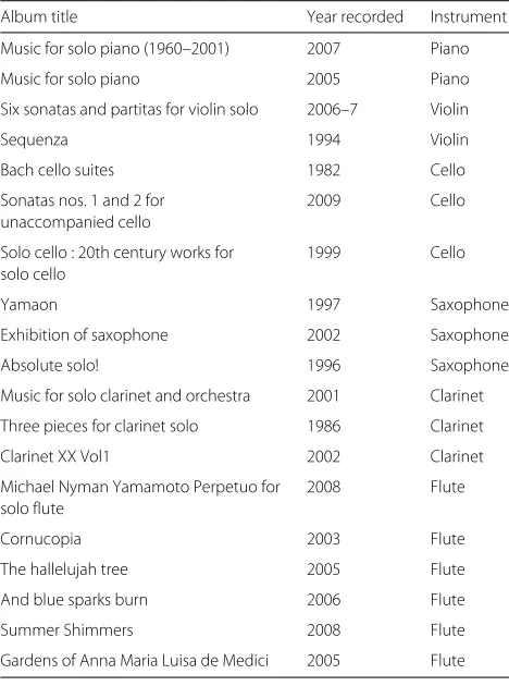
context of a solo performance. Here, we explore the short-term analysis of solo pieces and their correspondence to the musical timbre space, as well as a careful sampling of the musical phrase to best track the evolution of the musical phrase across notes and benefit from the learned knowledge based on isolated notes. We also investigate adaptive clustering techniques to map from one space to the other. In choosing solo musical performances, we focus on musical content from real world solo recordings obtained from commercial Compact Discs (CD) with no a priori screening.

Section 2 provides details about materials and methods used to setup our recognition system. These include the datasets used (subsection 2.1), approaches to parsing continuous solo recordings (subsection 2.2), method-ology for analyzing acoustic signals using STRF fea-tures (subsection 2.3) as well as the setup of training and testing our classifier (2.4). The evaluation section 3 details the outcome of instrument-recognition experi-ments using isolated notes, musical phrases in a mixed training/testing setup using both STRF features and com-parative approaches. A number of follow-up analyses follow in subsection 3.4 to investigate tests using artifi-cial datasets and various feature sets that shed light on the nature of the discrepancy in musical timbre charac-teristics between isolated notes and continuous phrases. Subsection 3.5 directly estimates the degree of mismatch between these two datasets using information theoretic measures. Finally, subsection 3.6 proposes a potential resolution to the issue of mismatch by using adaptive classification techniques that circumvent the divergence in statistical characteristics between the two datasets. A discussion (section 4) summarizes the main findings of the study and remarks on the empirical findings regarding cross training from isolated to continuous notes.

2 Materials and methods

2.1 Datasets

2.2 Parsing solo recordings

In dealing with continuous solo recordings, the musical phrase needs to be properly segmented. Here, we explore two possible techniques: (1) a uniform windowing technique where each audio is segmented into non-overlapping regions of durationτw; (2) a note extraction procedure that identifies the possible transitions between notes in the musical phrase. Both approaches are detailed next.

2.2.1 Windowing segmentation

The windowing approach is the least computationally costly technique to process a continuous recording. It involves segmenting the signal into non-overlapping win-dows of duration τw, which are subsequently analyzed through the cortical model to yield a spectrotemporal rep-resentation of the signal, averaged over its duration τw. This method ignores the occurrences of notes or chords and treats each segment equally. The window duration, τw, is a parameter that controls the time span of the fea-tures extracted from the signal, and can therefore play a crucial role in matching the features from solo perfor-mances relative to features extracted from isolated notes. The final choice of window durationτwused in the cur-rent work is found empirically by choosing the duration that yields that best recognition performance across our solo and RWC datasets (see section 3).

2.2.2 Harmonicity-based segmentation

The alternative way to a uniform sampling of the solo per-formances is to extract the individual notes in the phrase itself. Traditionally, the task of note extraction is often morphed into a task of onset detection, where a note is defined as the region between two onsets. Onsets are caused by a break in the steady state nature of a note, and onset detection involves evaluating a given audio signal using an onset detection function and applying certain selection criteria to decide the onset times. Phase devia-tion features have been widely used to detect departure from steady state behavior of a note, and hence, suc-cessfully applied to onset detection [31, 32]. However, onset-based techniques are quite sensitive to signal level characteristics which are easily affected by changing con-ditions like recording instruments and environments. They also require tedious tuning of parameters and thresholds for detecting transitions that vary greatly across databases [31]. Applying this approach in the current work is indeed challenging given the uncon-trolled nature of the commercial CD recordings used here requiring different tunings of thresholding criteria on a per recording basis.

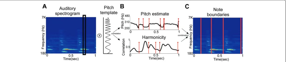
Instead, we opt for a harmonicity-based parsing method. Each note is typically characterized by a region of relatively steady pitch and significant harmonicity level.

Here, we use this steady-state information to identify regions of stable pitch frequency and high harmonicity. The analysis starts by a pitch estimation using a template matching approach as proposed by Goldstein et al. [33]. The spectrum (or spectral slice of the spectrogram) at any given time frame is compared to an array of pitch tem-plates. These templates represent the auditory spectrum of a generic note at a particular fundamental frequency. Here, we generate pitch templates T(f;fp) as a cosine function modulated by a Gaussian envelope repeated at the integer multiples of a fundamental frequency fp as given by Eq. 1.

T(f;fp) =

n 2e−

_f−

nfp αθ(n)

2

cos(2πθ(n)

β (f −nfp)) (1)

where θ(n) = 1 + 0.7∗n is a shrinkage factor, α = 18.28 andβ = 26 are constants. We use 128 pitch tem-plates spanning 5.3 octaves; which gives a resolution of one template every half semitone. The spectral slice of the spectrogram at every given timey(t0,f)is compared

against the template at each pitch frequencyfpgenerating a range of correlation valuesρ(t0;fp). The template with the maximum match is chosen as the corresponding pitch value for the spectrum at timet0and the degree of match

captured by the harmonicity variableH(t)(see Eq. 2).

ρ(t;fp) = corr(y(t,f),T(f;fp))

P(t) = argmax fp

ρ(t;fp) (2)

H(t) = max fp

ρ(t;fp)

where y(t,f) is the spectrogram derived in Eq. 5 and corris Pearson’s correlation coefficient. The harmonicity H(t)indicates the degree of match to the template at the selected pitch valueP(t). Based on this metric, we define a transition between notes as the region with change of pitch over time, accompanied with a reduced harmonicity value (due to possible overlap between notes at the bound-ary or percussive components in the onsets of the notes such as the hammer in the piano or bow in the violin). We define note boundaries using both pitch and harmonicity functions by setting selection criteria.

Note boundaries are selected based on the pitch func-tionP(t)when the following condition is met:

|P(t)−mode{P(t−w),P(t−w+1) . . .P(t)}| ≥ τ1

(3)

where τ1 = 0.2 and w = 30ms. Note boundaries can

(which is normalized to be 0 mean and unit variance) when the following three criteria are satisfied:

H(t) ≤ H(k) , ∀k:t−w≤k≤t+w

H(t) ≤

n+w

k=n−mwH(k)

mw+w+1 −τ2 (4)

H(t) ≤ gμ(t−1)

wherem = w = 30ms,τ2 = 0.3,mu = 0.1, andgμ(t) = min(H(t),μgμ(t−1)+(1−μ)H(t)).

Finally, the actual segmentation boundaries are selected as those times where the potential boundaries based on both the pitch P(t) and harmonicity H(t) agree (with a tolerance of 40 ms) (Fig. 1).

The note segmentation method described above is not error proof. One of the main sources of erroneous pars-ing of the solo recordpars-ings in the presence of simulta-neous notes (i.e., chords). Chords cause the harmonicity estimate to yield a large number of shorter segments with relatively stable pitches. To deal with this potential source of error, we confine our analysis to notes extracted that are longer in duration than a minimum threshold τn, defined empirically based on classification accuracy (see section 3). We also contrast the harmonicity-based segmentation described here to an onset-based method commonly used in the literature. Here, we test the “Rec-tified Complex Domain” (RCD) approach proposed by Dixon [31]. This onset-detection method is implemented as described in the publication with a 2048 hamming win-dow and shift of 441 sample (corresponding to 46 ms at a sampling rate of 44100 Hz). The Short Term Fourier Transform uses a shift of 10 ms. The onsets from the RCD function are calculated using the parameters suggested in the paper (ω=3,m=3,δ=0.5 andα=0, see [31]).

It is important to note that the harmonicity-based method described here is not a complete note segmen-tation approach in its own right. The technique simply relies on the steady-state behavior of pitch information that is typical in each musical note, and detects changes in this steady-state character in order to delimit poten-tial transitions to a new note. It does not carefully track

onsets and offsets of each note nor is it able to prop-erly parse irregular patterns such as instruments with long attack times (e.g., flute). It is likely that harmonicity does complement a number of signal-based techniques (using envelope or phase information) to provide a more robust acoustic-based partitioning of a solo musical phrase.

2.3 The STRF feature space

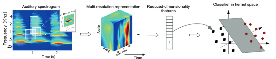
All signals are analyzed using a model developed to explore the neural underpinnings of musical timbre [17]. The model performs a decomposition of the spectro-temporal modulations of the acoustic signal. Modulations reflect the “changes" or variations in the spectral profile (e.g., peaks, troughs, center of gravity, smoothness of the spectrum) as well as “changes” or variations in the tempo-ral structure (e.g., rise and fall of the tempotempo-ral envelope, onsets, periodicity patterns). This level of detail results in a intricate analysis of the signal characteristics in a multi-resolution mapping, believed to mimic the filtering properties reflected by neurons in primary auditory cor-tex. Here, we review the key transformations in the model and point readers to [17, 34] for further details. Figure 2 depicts a schematic of the key stages in the model.

The initial stage of the model maps the one-dimensional acoustic waveform x(t) onto a two-dimensional time-frequency representation y(t,f). This transformation starts by convolving x(t) with a bank of 128, highly asymmetric, constant-Q filtersh(t,f)organized on a log-arithmic axis spanning 5.3 octaves. This stage models spectral filtering at the level of the cochlea and is fol-lowed by additional spectral sharpening modeled as a derivative along the frequency axis, and subsequently by a half wave rectification. Finally, the loss of phase lock-ing at the midbrain level is modeled as a low pass filter L(t,τ) = e−(τt)u(t), whereu(t) is the step function and τ = 4ms is a time constant. These transformations yield a two-dimensional auditory spectrogram that is fur-ther enhanced using a cubic root compression to boost low amplitude events and transitions (Eq. 5). This spec-trographic representation of sound tracks the spectral

Fig. 2Schematic of the STRF-based instrument classification. Schematic of the processing stages involved in the STRF-based model of instrument classification. A time-frequency spectrogram is derived for each acoustic signal, then further mapped onto a higher dimensional space using an STRF-based model. The STRF space is then reduced in dimensionality and mapped via a kernel function to a new space to define boundaries between different musical instruments

profile of the signal as well as the temporal “envelope modulations” due to interactions between spectral com-ponents that fall within the bandwidth of each filter. The frequencies of these modulations are naturally limited by the maximum bandwidth of the cochlear filters. The resultant auditory spectrogram can be easily replaced by other time-frequency representations (e.g., Short-Term Fourier Transform, Slaney’s Gammatone toolbox spectro-gram [35], etc). The biologically-inspired representation chosen in the current study (Eq. 5) has been shown to exhibit interesting properties such as self-normalization and robustness [36].

y(t,f)=max(∂fx(t)⊗th(t,f), 0)⊗tL(t,τ) 1

3 ₍₅₎

The next stage further decomposes components of the spectrogram through a bank of modulation-tuned filters G, selective to specific ranges of modulation in time (rates rin Hz) and in frequency (scalessin cycles/octave), called STRFs (spectro-temporal receptive fields). The STRF fil-ters are defined by:

G+(t,f;r,s) = A∗(hr(t;r))A(hs(f;s)) (6)

G−(t,f;r,s) = A(hr(t;r))A(hs(f;s))

whereA(.)indicates an analytic function,(.)∗is complex conjugate, and+/−indicates upward or downward ori-entation selectivity in time-frequency space (i.e., detecting upward or downward frequencies sweeping over time). The use of the analytic and complex conjugate pairing ensures that the receptive field are complex functions that share quadrant-separability properties observed in physi-ological data. In other words, these wavelet functions are not a simple separable product of a spectral and a tem-poral function (see [34] for further discussion). The seed functionshr(t)andhs(f)are shaped as Gamma and Gabor functions respectively, as given in Eq. 7.

hr(t)=t3e−4tcos(2πt) , hs(f)=f2e1−f2 (7)

and their scaled versions are given byhr(t;r) = rhr(rt) andhs(f;s)=shs(sf).

The final output of this STRF-based analysis is then a four-dimensional complex-valued representation along timet, frequencyf, temporal modulationsrand spectral modulationss; given by:

Z(t,f;r,s)=y(t,f)⊗t_,f G(t,f;r,s) (8)

In the current study, we use 11 temporal rates equally spaced on a logarithmic axis from 4 to 125 Hz in both upward and downward directions, and 11 spectral scales equally spaced on a logarithmic axis from 0.25 to 8 cycles/octave. We also average the magnitude of the mod-ulation representation Z along time over the duration of the signal (i.e., entire musical note in case of RWC databaset) or analysis window (see discussion of choice of time window below), and further reduce the dimension-ality of the 22x11x128 STRF tensor to a 420 dimensional vectorXiusing tensor singular value decomposition [37] preserving 99.9 % of the variance along each dimension. It is important to note that instead of analyzing the signal over short-time windows and maintaining a time series representation over all windows, the current approach averages across the entire duration of the signal being ana-lyzed and maintains only average statistics. While time is not explicitly represented, it is implicitly captured via the temporal modulation axis (r) which captures how the signal changes over time, hence effectively encoding information about the temporal envelope of each spectral component in the acoustic waveform.

2.4 Recognition setup

Finally, the reduced-dimensionality feature vector Xi ∈

R420_{is combined with its instrument labelY}

i ∈(+1,−1) to form a training datasetD420= {(Xi,Yi)}Ni=1for a

J(X): R420 → {+1,−1}

J(Xi) = wTφ(Xi) (9)

Here,φ(.)is the radial basis kernel chosen for this study, and w is a linear decision boundary derived by optimizing the following function:

min

w 1

2||w||2+C

N

i=1ξi (10)

such that ξi≥0, YiwTφ(Xi)≥1−ξi, ∀(Xi,Yi)∈D420

C is a scalar cost factor and N_i=1ξi measures the total classification error. Essentially, the classifier identi-fies boundaries between classes of instruments. We train pairwise classifiers for every pair of instruments, and use the winner as the selected class across all pairwise com-parisons. In the current work, the training and testing data are extracted from one of three possible sets: (1) matched setting: both training and testing data are from the same database (either RWC or solo recordings parsed in a spe-cific manner); (2) cross-domain setting relative to RWC: the training data for the classifier is defined from RWC notes while the testing data is extracted from a parsing of the solo recordings; (3) cross-domain setting relative to solo: the training data is compiled from a parsing of the solo recordings while the testing is performed on the RWC notes. In the matched setting, we use different data subsets for training and testing. In all cases, we per-form a grid search to tune the optimal choice of classifier and kernel parameters, and use a ten-fold cross-validation to evaluate the performance of the system. Accuracy is defined as the sum of correctly classified examples from all instruments divided by total number of examples from all instruments. Examples refer to solo notes, windows or isolated notes, depending on the specific experiment. All instruments were given equal weight in this computation.

3 Evaluation

3.1 Uniform windowing of solo recordings

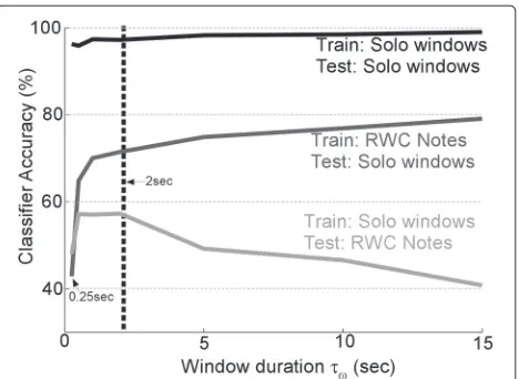
In order to determine the optimal choice of uniform window lengthτwfor parsing the solo recordings, we per-formed three sets of recognition experiments based on a matched setting (train on solo, test on solo) and cross-domain setting (train on solo, test on RWC or train on RWC, test on solo). The RWC notes are analyzed one note at a time (averaged over the entire duration of the note), while the solo recordings are parsed into segments of length τw then analyzed through the receptive field model. Figure 3 shows the tradeoff between short and long-term spans of the analysis windowτw, as a function of accuracy of our recognition model. The best perfor-mance is achieved in a matched context where training and testing is done on a uniform set of segmented solo windows. In this case, the classifier quickly saturates as τw grows from as low as 250 msec to few seconds and

Fig. 3Recognition accuracy using uniform windowing of solo performances. Accuracy for uniform windowing experiments in matched and cross-domain train/test settings of continuous solo phrases as a function of window sizeτw

seems to depend very little of the value ofτw. In contrast, training and testing with a mismatched dataset is greatly affected by the window duration. Training on RWC notes and testing on solo segments quickly improves for short segments and hovers between 70–80 % accuracy with a monotonic increase. In the opposite setting, training on solo segments with very short windows (e.g., 250 msec) or too long windows seems to greatly affect the performance. Shorter segments likely capture too much variability in the instrument’s time profile hence producing inconsis-tencies in the features learnt from each class, for instance confounding the transient and steady-state nature of the signal. Longer windows excessively average the temporal profile of each instrument making it harder to distin-guish from instruments with comparable spectral profiles. A balance between short-term and long-term averaging appears to peak around 2 s. In the current study, we choose τw = 2 s as our optimal choice for all future experiments. Clearly, this choice can be optimized for dif-ferent applications, and is likely affected by the diversity in the solo database used. It may also be slightly biased by the comparison with the RWC database, whose notes are on average 2.7 s in duration, though they varied between 0.1–18 s.

3.2 Harmonicity parsing of solo recordings

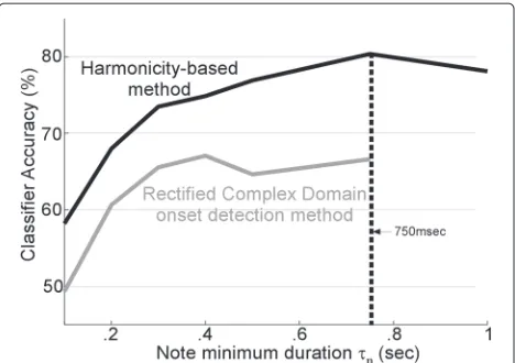
Fig. 4Harmonicity-based note extraction accuracy. The plot depicts the accuracy of the classifier on isolated notes extracted using a harmonicity-method, as a function of minimum note durationτn. This

method is contrasted with an onset-based method (the rectified complex domain, by Dixon [31]) for note extraction from musical phrases

around 750 msec before it starts dropping again. The opti-mal choice of 750 msec is not necessarily reflective of a fundamental tempo or window size in the data. Rather, it is constrained by the total amount of data we have available for our solo recordings database. Constraining the note to be of a certain duration limits the num-ber of notes we have available in the database. Based on the performance of the note extraction shown in Fig. 4, we choose 750 ms as the value ofτnfor all future experiments. Overall, the harmonicity-parsing algorithm suggests that our selection of solo CDs include an aver-age of 7569 notes per instrument with mean duration of 0.44 s and median of 0.26 s per note (ranging from 0.1 to 4.85 s).

We also contrast the harmonicity-based method with other note extraction techniques from the literature based on onset-detection. Figure 4 overlays the perfor-mance of the same support vector classifier optimized for notes extracted based on onset-detection following the Rectified Complex Domain approach proposed by Dixon [31]. As is evident from the classification results, the pitch-harmonicity measure allows for more accurate identification of musical instruments for all values ofτn, irrespective of pruning based on acceptable note size.

3.3 Instrument recognition results

To fully explore the relevance of the modulation feature space in capturing informative characteristics of musical timbre, we use the model with the chosen solo parsing parameters (for uniform windowing and harmonicity-parsing) to test classification accuracy in a matched and domain setting. Table 1 shows a ten-fold cross-validation contrasting three classifiers, each trained on

Table 1Results of cross-testing instrument recognition using STRF feature space

Train\test RWC Notes Windows

RWC 98.5±0.2 % 78±2.1 % 71±1 %

Notes 44.7_±0.9 % 97.7_±0.6 % 93.4_±0.5 %

Windows 58.5_±1.5 % 97.3_±0.5 % 96.9_±0.4 %

one of the three sets (RWC, harmonicity-parsing notes and uniform windows). All three sets yield a high per-formance above 97 % in a matched training-testing. The performance drops when a mismatched set is used for training and testing.

Taking a close look at the results from Table 1, we note that the mixed training/testing on solo recordings using uniform windows or segmented notes reveal a high degree of agreement across both methods. The higher accuracy for the harmonicity-parsing technique as compared to the uniform windowing technique when tested against a clas-sifier trained on RWC notes indicates that note extraction based on harmonicity was better at reducing the differ-ence between the datasets. This result is not surprising since the RWC dataset also has isolated notes. Finally, the low classification accuracy for the classifiers trained on the feature sets derived from solo music database when tested on RWC database indicates that RWC database is a more generalized database with much more vari-ance in the data as compared to the solo music database collected for the current study. This outcome could poten-tially be improved with inclusion of a larger dataset of solo recordings.

Table 2Results of cross-testing instrument recognition using MPEG7-based spectral features

Train\test RWC Notes Windows

RWC 62.2±1.0 % 51.0±1.4 % 43.1±1.0 %

Notes 41.3_±1.3 % 79.3_±1.4 % 70.3_±0.7 %

Windows 38.6_±1.8 % 81.4_±1.3 % 78.4_±0.9 %

these MPEG7-based features. While this drop in perfor-mance is not a definitive statement of the superiority of the STRF approach, it reflects that these two methods capture different levels of granularity in the signal, which provide different sets of informative features to a back-end classifier.

In a separate experiment, we investigate how the classification system with solo recordings behaves with “unseen” data. We extract note segments from all but one CD (selected at random for each instrument) using the harmonicity-based parsing approach. This data is then divided into a 90 % training set and 10 % testing set (homo-geneous test). The same classifier trained on 90 % of the data is tested again with data from the left out CD (het-erogeneous test). Table 3 summarizes the classification results using both STRF and MPEG7 features. Using both feature sets, the performance does drop, though in a more dramatic fashion in the case of MPEG7 features. Note that the CD selection was not pre-screened in any way, and the selection included a wide range of recording settings and playing styles that are difficult to capture when train-ing on a small number of CDs (as little as 1 CD in case of piano for example). Nevertheless, the accuracy remains at a high level that could certainly be strengthened with enough diversity in the training set.

Finally, we perform an additional experiment to explore the contribution of different acoustic features. Our earlier study [17] explored the contribution of both spectral and temporal dimensions; and has indeed confirmed that the use of joint spectro-temporal modulation fea-tures is key to fully accounting for the multidimensional nature of musical timbre in isolated notes, in agreement with earlier findings in the literature [20]. To comple-ment these previous observations, we compute the per-formance of our classifier on RWC notes as well as isolated solo notes using the harmonicity-based parsing approach with varying combinations of acoustic features

Table 3Classification results using homogeneous training/ testing or heterogeneous (leave one CD out) conditions

Features Homogeneous test Heterogeneous test

STRF features 97.7±0.6 % 88.1±0.5 %

MPEG7 features 80.0_±2.4 % 66.1_±0.6 %

(frequency, scale, and rate). Table 4 shows the classifier accuracy for different feature combinations. The results confirm a number of observations: (1) frequency is an important dimension in defining instrumental timbre; (2) augmenting the frequency axis with rate or scale dimensions provides improvement to the classifier accu-racy; (3) including all three dimensions of rate, scale, and frequency further improves the accuracy results on solo notes.

3.4 Follow-up analyses

We run follow-up tests to better understand the corre-spondence between isolated notes and notes in contin-uous solo performances. These follow-up analyses use artificial datasets recreated from the datasets used in the main study. First, we create a new dataset by concate-nating notes along time from RWC database in order to simulate the succession of notes in a solo musical phrase. To determine the number of notes to be concatenated, we compute a histogram of the number of notes that are extracted from 2-s segments. The histogram yields the values [58, 32, 8.5, 1, and 0.5 %] where the first num-ber indicates the ratio of single notes, the second indicates the number of times two notes were extracted and so on. An artificial dataset with 2000 samples per instrument class is then created by concatenating the required num-ber of notes, randomly selected, to match this histogram. We then train a classifier on this artificial set and test on uniform windows from solo music dataset. This experi-ment yields an accuracy of 71.76 %. The lack of significant improvement, when compared to the model trained on RWC notes (71.42 %), suggests that artificial concatena-tion of isolated notes does not recreate the transiconcatena-tion characteristics between notes in a musical performance, and hence provides no further improvement in matching uniform solo segments with isolated notes from RWC.

Table 4Classification results with matched training/testing using different acoustic features

Rates (22dim) Scales (11dim) Freq (128dim) RateScale (242dim) ScaleFreq (420dim) RateFreq (420dim) RateScaleFreq (420dim)

RWC 73.3±1.2 % 57.5±0.9 % 93.5±0.7 % 93.8±0.8 % 97.7±0.4 % 97.5±0.5 % 98.5±0.2 %

Notes 69.6_±1.9 % 67.0_±1.9 % 93.0_±0.9 % 90.0_±0.6 % 96.0_±0.8 % 96.1_±1.1 % 97.7_±0.5 %

the existence of few chords in the parsing of solo phrases is likely a negligible factor in explaining the mismatch between the two datasets. Indeed, the solo CDs used in our current analysis contain very few instances of chords. An informal listening test indicates that less than 5 % of the notes are chords. A more careful analysis using anno-tated musical performances will be needed to formally assess the effect of chords on instrument recognition in isolated vs. solo phrases. In the datasets used in the cur-rent study, chords appear to be an insignificant factor in explaining the mismatch between isolated and continuous notes.

Finally, to further investigate the mismatch between isolated notes and musical phrases in the temporal domain, we leave out temporal information in the STRF feature space by averaging the temporal modulation axisr) and only maintaining the scale-frequency dimen-sions z(f;r,s). These spectral-only features are then used to test a recognition system trained on notes extracted from solo recordings (using the harmonicity approach) and tested on isolated notes. This experiment yields an accuracy of 43.3 % (compared to 44.7 % when trained with full STRF features—see Table 2). Discarding tempo-ral information does not seem to have a notable impact on the classification accuracy. This minimal change in accu-racy score suggests that the mismatch (or lack thereof ) of temporal characteristics between solos and isolated notes does not explain the accuracy of 44.7 % when testing on isolated notes. This low accuracy may be due to other factors (e.g., inaccuracy in parsing notes from solo sig-nals, differences in transient or steady-state behavior of

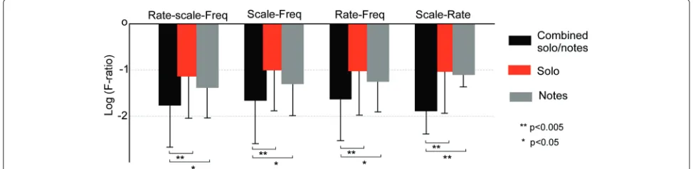
notes in a phrase which alters their spectral character-istics, or complete mismatch in temporal characteristics which causes no difference whether a temporal axis is included in the feature set or not). We confirm this obser-vation by analyzing the homogeneity of different instru-ment classes using different acoustic attributes. To do so, we use the F-ratio (an extension of Fisher’s discrim-inant [41]) to assess discriminability across instrument classes [42]. Fisher’s discriminant classically operates on a two-class problem and measures the difference between the means or centroids of two classes relative to their variances. The F-ratio extends this definition to a multi-class problem. It is defined as the variance of means (between class) / mean of variances (within class). We combine a dataset using (randomly chosen equal por-tions of ) solo windows and isolated notes and compute the F-ratio using rate-scale-frequency vs. scale-frequency features. The results highlight that combining the two datasets increases instrument mislabeling, hence signifi-cantly reducing class discriminability which is indicative of higher heterogeneity across the two datasets (Fig. 5). Moreover, in agreement with the classification outcome, the mean log F-ratio (we take the log value to highlight lower F-ratios) using rate-scale-frequency is −1.8± 0.7 while that using scale-frequency is −1.7 ±0.7. Clearly, dropping the rate information does not significantly affect the separability across instruments when comparing a combined dataset of solo and isolated notes. In con-trast, the same feature set (rate-scale-freq) appears to be more discriminative (higher average F-ratio) for more homogeneous datasets using solo or isolated notes by

themselves (Fig. 5). Overall, an analysis of discriminability of rate, scale, and frequency features over individual datasets (solo, RWC) shows a higher separability of instru-ment classes within each dataset. In order to shed light on the heterogeneity of the feature space across solo and isolated notes, one has to take into account the sources of variability in the combined dataset, as analyzed next.

3.5 Discrepancy between datasets

In an attempt to directly estimate the differences between the isolated notes and solo recordings datasets, we compute the balanced Kullback-Leibler (KL) diver-gence [43] on distribution of features z(f;r,s) for each instrument extracted from the two databases. The KL metric is a comparison of two probability distri-butions of a given instrument from both databases; defined as:

KL(p1,p2)=

x

p1(x)log p1(x) p2(x)+

p2(x)log p2(x) p1(x)

(11)

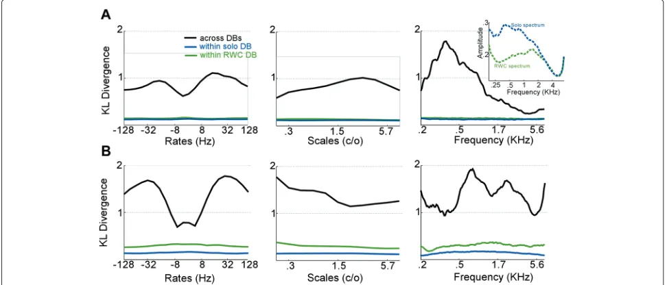
This comparison gives us a better insight into the the main areas of mismatch between isolated notes in RWC dataset and notes extracted from the continuous recordings. We analyze this distance metric for each point along the three-dimensional space of rate-scale-frequency. Figure 6 shows the KL divergence averaged along each of the three dimensions for piano notes (Fig. 6a) and flute notes (Fig. 6b). For completeness, we compute KL divergence within pairs of signals from each

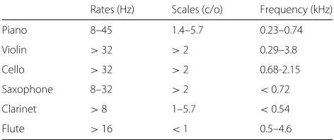
database (RWC or solo performances) as well as compar-ing the two databases. As expected, the within database KL values are much lower and consistent across datasets suggesting a higher degree of consistency within the data from each set. In contrast, the RWC and solo notes show high degrees of disagreement at specific parts of the space depending on the instrument. For instance, the piano RWC and solo notes show greater discrepancy at lower frequency (< 1KHz). Examining the average spec-trum from each database (inset in rightmost panel in Fig. 6a) confirms a different spectrum roll-off between the two datasets; which could be explained by a num-ber of “music”-related factors such as resonance emphasis or “non-music”-related factors such as recording environ-ment and channel distortions. Note that both datasets were pre-emphasized using a highpass filter with param-eters [ 1,−0.97]). In contrast, the flute reveals a higher mismatch in the mid-high frequency range as shown in Fig. 6b, rightmost panel. Table 5 summarizes the regions of high divergence between the two datasets for all the instruments. This result highlights that discrepan-cies between the two datasets are not due to a systematic mismatch; but is rather instrument dependent. Teasing apart the causes of mismatch is not a straightforward endeavor. It could be due to many factors, including differ-ences in recording instruments, room acoustics, channel noise, signal postprocessing and filtering emphasis, etc. A number of musical reasons could also contribute to this mismatch; notably due to the expressivity or transi-tions between notes in real recordings in contrast with

Table 5Regions of high mismatch between the RWC and solo datasets

Rates (Hz) Scales (c/o) Frequency (kHz)

Piano 8–45 1.4–5.7 0.23–0.74

Violin _>32 _>2 0.29–3.8

Cello _>32 _>2 0.68-2.15

Saxophone 8–32 _>2 _<0.72

Clarinet >8 1–5.7 <0.54

Flute >16 <1 0.5–4.6

isolated notes. Next, we explore a method to overcome the difference in distributions across instruments.

3.6 Adaptive cross-domain classifier

It is clear from the control and statistical analysis that the average profile distributions of segments from the solo and RWC databases play an important role in justifying the classification mismatch between the two datasets. In order to circumvent this divergence in signal properties, we investigate the use of an adaptation technique to adjust the support vector machine boundaries between instru-ments based on a first database to the new statistical profiles of a second different database using an adaptive SVM technique. When using RWC as our baseline train-ing set, the current classifier learns a decision function JRWC_{(X)based on the profile of dataXfrom the RWC} notes (Eq. 9). In order to conform better to the statis-tical structure of the solo dataset, we use an improved cross-domain classifier, called an adaptive support vector machine. Essentially, a new decision function is learned, defined as:Jsolo(x)= JRWC(x)+J(x)where the new decision function follows a similar minimization proce-dure as a typical support vector machine classifier (Eq. 10) but with an added constrain to minimize the update term J(x). This ensures that the decision boundary is kept as a close as possible to the original RWC-trained classi-fier. Details of the adaptation follow the exact procedure outlined in [44], using software provided by the authors of this work. By leveraging the knowledge from the available RWC database, this method makes small adjustment to the decision weight in feature space to accommodate the different distribution in the solo music. This procedure requires using small training data from the solo dataset. Without any adaptation, the support vector machine clas-sifier trained on RWC and tested on solo recordings parsed using the harmonicity method yields an accuracy of 78 % (Table 2). We use 200 randomly selected notes from the solo music dataset per instrument as the adap-tation set to adjust the decision boundary and retest the classifier with a separate set of solo segments (i.e., about 3–5 min of solo data). The performance of the model

after adaptation is found to be 86.6 % indicating that we can successfully adapt a model trained on one dataset to another condition under limited data constraints. For this adaptation, we set the value of the cost parameter (C) to be 1 which was found to maximized the average performance across both solo music dataset and RWC notes.

4 Discussion and conclusions

The current work pursues the goal of musical instrument identification in continuous recordings. This problem combines the issue of both musical timbre recognition as well as dealing with the potential mismatch between readily available single music note data and continuous recordings. As is common in most systems of automated sound recognition, these issues translate to: (1) choos-ing appropriate signal characteristics and sound features that are most informative about the instrument class; (2) determining the relevant temporal context (e.g., choice of windowed analysis of the signal); and (3) adopting the proper statistical representation for correctly classifying the data.

While the applicability of such STRF features for contin-uous solo performances is remarkably accurate, the cross-domain transition from single notes to musical phrases (even for solos) is not a trivial one. As our analysis shows, the classic windowing approach to parse musical phrases is suboptimal [23, 26, 28, 53]. It coarsely bins the time signal into segments of equal length; but with no con-sideration to the underlying structure. A more effective way is to provide a better match to the composition of the musical phrase; by attempting a pitch-based parsing of individual notes. Ultimately, the recognition of musi-cal instruments in continuous recordings is a delicate balance of acoustic, musical, and environmental factors. On the one hand, the physical attributes of each musical instrument color its sound with unique spectro-temporal features. These are best extracted by a rich enough fea-ture set. On the other hand, the constrains of the musical genre, the melodic rhythm as well as the non-musical constrains (e.g., recording environment, choice of physi-cal instrument, playing style, signal preprocessing) greatly shape the characteristics of the signal and ultimately the true match of the instrument’s identity. An analysis of KL-divergence between the RWC single notes database and the off-the–shelf solo CDs used in the current study highlights that differences are not feature specific (time vs. frequency) or instrument specific (Table 5). In addition, our follow-up analyses show that discrepancies in train-ing/testing across datasets cannot be simply explained by issues with the parsing method such as note sequence structure or presence of chords. In order to best miti-gate the divergence in statistical characteristics between the two datasets, the current work proposes the use of adaptive classification methods that maintain the struc-ture of a model trained on isolated notes but regulate their decision boundary to capture diverging proper-ties from continuous musical phrases. The use of this adaptive approach provides an improvement in recogni-tion accuracy of about 6 % with very minimal training data using less than 5 min of additional data from the solo dataset.

Overall, while a true instrument identification system would have to carefully account for cross-referencing a variety of datasets [54], the current study sheds some light on the applicability of a rich STRF feature space and adaptive machine learning techniques. The exploration of different levels of abstraction could be greatly infor-mative in addressing the mapping from single notes to continuous recordings. Considering the temporal place-ment of notes in the context of the entire musical phrase as well as para-timbral information could greatly inform the identification of the musical instrument; though it would take the system from a purely acoustic-driven analysis to a more data mining and information retrieval approach.

Appendix

Table 6List of sources in the solo music database

Album title Year recorded Instrument

Music for solo piano (1960–2001) 2007 Piano

Music for solo piano 2005 Piano

Six sonatas and partitas for violin solo 2006–7 Violin

Sequenza 1994 Violin

Bach cello suites 1982 Cello

Sonatas nos. 1 and 2 for 2009 Cello

unaccompanied cello

Solo cello : 20th century works for 1999 Cello solo cello

Yamaon 1997 Saxophone

Exhibition of saxophone 2002 Saxophone

Absolute solo! 1996 Saxophone

Music for solo clarinet and orchestra 2001 Clarinet

Three pieces for clarinet solo 1986 Clarinet

Clarinet XX Vol1 2002 Clarinet

Michael Nyman Yamamoto Perpetuo for 2008 Flute solo flute

Cornucopia 2003 Flute

The hallelujah tree 2005 Flute

And blue sparks burn 2006 Flute

Summer Shimmers 2008 Flute

Gardens of Anna Maria Luisa de Medici 2005 Flute

Competing interests

The authors declare that they have no competing interests.

Acknowledgements

This work is supported by grants from the NSF grant IIS-0846112, NIH grant 1R01AG036424, ONR grants N00014-12-1-0740, and N000141010278.

Received: 29 January 2014 Accepted: 2 September 2015

References

1. HV Helmholtz,On the sensations of tone, second edition. (Dover Publications, 1954)

2. A Preis, An attempt to describe the parameters determining the timbre of steady-state harmonic complex tones. Acustica.55(1), 1–113 (1984) 3. S McAdams, S Winsberg, S Donnadieu, GD Soete, J Krimphoff, Perceptual

scaling of synthesized musical timbres: common dimensions, specificities, and latent subject classes. Psychological Research.58(3), 177–192 (1995) 4. S Samson, RJ Zatorre, JO Ramsay, Multidimensional scaling of synthetic

musical timbre: perception of spectral and temporal characteristics.51(4), 307–315 (1997)

5. WH Lichte, Attributes of complex tones. J. Exp. Psychol.28, 455–481 (1941) 6. G von Bismarck, Sharpness as an attribute of the timbre of steady sounds.

Acustica.30, 159–159172 (1974)

7. JM Grey, Multidimensional perceptual scaling of musical timbres.61(5), 1270–1277 (1977)

8. JM Grey, An Exploration of Musical Timbre, Ph.D. dissertation,Department of Psychology, Stanford University (1975)

10. J Risset, D Wessel, inExploration of timbre by analysis and synthesis, ed. by D Deutsch. The psychology of music (Academic Press, New York, 1982), pp. 25–2558

11. W Strong, M Clark, Synthesis of wind instrument tones. J. Acoust. Soc. Am.

41(1), 39–52 (1967)

12. D Luce, Physical correlates of nonpercussive musical instrument tones, Ph.D. dissertation,Department of Physics, Massachusetts Institute of Technology (1963)

13. E Saldanha, J Corso, Timbre cues and the identification of musical instruments. J. Acoust. Soc. Am.36(11), 2021–2026 (1964) 14. S McAdams, inThinking in sound: The cognitive psychology of human

audition, ed. by S McAdams, E Bigand. Recognition of sound sources and events (Oxford University Press Oxford, 1993), pp. 146–198

15. I Borg, P Groenen,Modern multidimensional scaling: theory and applications, Second edition. (Springer, 2005)

16. J Krimphoff, S McAdams, S Winsberg, Caracterisation du timbre des sons complexes. ii : Analyses acoustiques et quantification psychophysique. J. Physiol.4(C5), 625–628 (1994)

17. K Patil, D Pressnitzer, S Shamma, M Elhilali, Music in our ears: the biological bases of musical timbre perception. PLoS Comput. Biol.8(11), 1002759 (2012)

18. JM Grey, Timbre discrimination in musical patterns. J. Acoust. Soc. Am.

64(2), 467–472 (1978)

19. RA Kendall, The role of acoustic-signal partitions in listener categorization of musical phrases. Music. Percept.4(2), 185–213 (1986)

20. P Herrera-Boyer, G Peeters, S Dubnov, Automatic classification of musical instrument sounds. J. New Music Res.32(1), 3–21 (2003)

21. JC Brown, Computer identification of musical instruments using pattern recognition with cepstral coefficients as features. J. Acoust. Soc. Am.

105(3), 1933–1941 (1999)

22. A Eronen, A Klapuri, inproceedings of the IEEE International Conference on Acoustics, Speech, and Signal Processing. Musical instrument recognition using cepstral coefficients and temporal features, vol. 2, (2000), pp. 753–756. doi: 10.1109/ICASSP.2000.859069

23. A Eronen, inproccedings of the IEEE Workshop on Applications of Signal Processing to Audio and Acoustics. Comparison of features for musical instrument recognition, (2001), pp. 19–22. doi:

10.1109/ASPAA.2001.969532

24. JC Brown, O Houix, S McAdams, Feature dependence in the automatic identification of musical woodwind instruments. J. Acoust. Soc. Am.

109(3), 1064–1072 (2001)

25. S Essid, G Richard, B David, Instrument recognition in polyphonic music based on automatic taxonomies. IEEE Trans. Audio, Speech, and Lang. Process.14(1), 68–80 (2006)

26. A Azarloo, F Farokhi, inProceedings of the Fourth International Conference On Computational Intelligence, Communication Systems and Networks (CICSyN). Automatic musical instrument recognition using k-NN and MLP neural networks, (2012), pp. 289–294. doi: 10.1109/CICSyN.2012.61 27. DG Bhalke, CBR Rao, DS Bormane. Dynamic time warping technique for

musical instrument recognition for isolated notes, in proceedings of the International Conference On Emerging Trends in Electrical and Computer Technology (ICETECT), (2011), pp. 768–771. doi:

10.1109/ICETECT.2011.5760221

28. S Essid, G Richard, B David, Musical instrument recognition by pairwise classification strategies. IEEE Trans. Audio, Speech, and Lang. Process.

14(4), 1401–1412 (2006)

29. GE Hall, H Hassan, M Bahoura, inproceedings of the 11th International Conference On Information Science, Signal Processing and Their Applications (ISSPA). Hierarchical parametrisation and classification for musical instrument recognition, (2012), pp. 1039–1044. doi:

10.1109/ISSPA.2012.6310442

30. M Goto, H Hashiguchi, T Nishimura, R Oka, Rwc music database: Music genre database and musical instrument sound database. Proc. Int. Symp. Inf. Retr, 229–230 (2003)

31. S Dixon, inProceedings of the 9th International Conference on Digital Audio Effects. Onset detection revisited, (2006), pp. 133–137

32. JP Bello, L Daudet, S Abdallah, C Duxbury, M Davies, MB Sandler, A tutorial on onset detection in music signals. IEEE Trans. Speech and Audio Process.13(5), 1035–1047 (2005)

33. JL Goldstein, An optimum processor theory for the central formation of the pitch of complex tones.54, 1496–1516 (1973)

34. T Chi, P Ru, SA Shamma, Multiresolution spectrotemporal analysis of complex sounds. J. Acoust. Soc. Am.118(2), 887–906 (2005)

35. M Slaney,Auditory toolbox. Technical Report, Report 45. (Interval Research Corporation, Palo Alto, CA, 1994)

36. K Wang, SA Shamma, Self-normalization and noise-robustness in early auditory representations. IEEE Trans. Speech and Audio Process.2, 421–435 (1994)

37. LD Lathauwer, BD Moor, J Vandewalle, A multilinear singular value decomposition, SIAM Journal on Matrix Analysis and Applications.21, 1253–1278 (2000)

38. N Cristianini, J Shawe-Taylor,Introduction to support vector machines and other Kernel-based learning methods. (Cambridge University Press, Cambridge, UK, 2000)

39. E Benetos, M Kotti, C Kotropoulos, inProceedings of the IEEE International Symposium On Circuits and Systems (ISCAS). Musical instrument classification using non-negative matrix factorization algorithms, (2006), p. 4. doi: 10.1109/ICASSP.2006.1661252

40. H-G Kim, N Moreau, T Sikora, Audio classification based on mpeg-7 spectral basis representations. Circ. Sys. Video Tech. IEEE Trans.14(5), 716–725 (2004)

41. RO Duda, PE Hart, DG Stork,Pattern Classification. (Wiley, New York, NY, 2000)

42. K Cios, W Pedrycz, R Swiniarski, L Kurgan,Data mining: a knowledge discovery approach. (Springer, New York, NY, 2007)

43. T Cover, J Thomas,Elements of information theory. (Wiley-Interscience, New York, 2006)

44. J Yang, R Yan, A Hauptmann, inProceedings of the 15th International Conference on Multimedia. Cross-domain video concept detection using adaptive SVMs, (2007), pp. 188–197. doi: 10.1145/1291233.1291276 45. SM J A Burgoyne, inProceedings of the Computer MusicModeling and

Retrieval. A meta-analysis of timbre perception using nonlinear extensions to CLASCAL (Springer-Verlag Heidelburg, 2007), pp. 181–202. doi: 10.1007/978-3-540-85035-9_12

46. S Donnadieu, inAnalysis, Synthesis, and Perception of Musical Sounds, ed. by J Beauchamp. Mental representation of the timbre of complex sounds (Springer New York, 2007), pp. 272–319

47. M McKinney, J Breebaart, inInternational symposium on music information retrieval (ISMIR). Features for audio and music classification, (2003), pp. 151–158

48. A Lerch,An introduction to audio content analysis: applications in signal processing and music informatics. (Wiley-IEEE Press, Hoboken, NJ, 2012) 49. AM Leaver, JP Rauschecker, Cortical representation of natural complex

sounds: effects of acoustic features and auditory object category. J. Neurosci.30(22), 7604–7612 (2010)

50. K Siedenburg, P Depalle, inProceedings of the IEEE Workshop On Applications of Signal Processing to Audio and Acoustics (WASPAA). Modulation filtering for structured time-frequency estimation of audio signals, (2013), pp. 1–4. doi: 10.1109/WASPAA.2013.6701863 51. JJ Burred, From sparse models to timbre learning: new methods for

musical source separation, doctoral dissertation, University of Berlin (2009) 52. E Hall, H Ezzaidi, M Bahoura,Advanced Machine Learning Technologies and

Applications, vol. 322. (A Hassanien, A Salem, R Ramadan, T Kim, eds.) (Springer, Berlin Heidelberg, 2012), pp. 152–152161

53. AG Krishna, TV Sreenivas, inProceedings of the IEEE International Conference on Acoustics, Speech, and Signal Processing (ICASSP). Music instrument recognition: from isolated notes to solo phrases, vol. 4, (2004), pp. 265–268. doi: 10.1109/ICASSP.2004.1326814