ORIGINAL ARTICLE
Vibration Performance Analysis
of a Mining Vehicle with Bounce and Pitch
Tuned Hydraulically Interconnected Suspension
Jie Zhang
1, Yuanwang Deng
1*, Nong Zhang
2, Bangji Zhang
1, Hengmin Qi
1and Minyi Zheng
3Abstract
The current investigations primarily focus on using advanced suspensions to overcome the tradeoff design of ride comfort and handling performance for mining vehicles. It is generally realized by adjusting spring stiffness or damp-ing parameters through active control methods. However, some drawbacks regarddamp-ing control complexity and uncertain reliability are inevitable for these advanced suspensions. Herein, a novel passive hydraulically intercon-nected suspension (HIS) system is proposed to achieve an improved ride-handling compromise of mining vehicles. A lumped-mass vehicle model involved with a mechanical–hydraulic coupled system is developed by applying the free-body diagram method. The transfer matrix method is used to derive the impedance of the hydraulic system, and the impedance is integrated to form the equation of motions for a mechanical–hydraulic coupled system. The modal analysis method is employed to obtain the free vibration transmissibilities and force vibration responses under different road excitations. A series of frequency characteristic analyses are presented to evaluate the isolation vibra-tion performance between the mining vehicles with the proposed HIS and the convenvibra-tional suspension. The analysis results prove that the proposed HIS system can effectively suppress the pitch motion of sprung mass to guarantee the handling performance, and favorably provide soft bounce stiffness to improve the ride comfort. The distribution of dynamic forces between the front and rear wheels is more reasonable, and the vibration decay rate of sprung mass is increased effectively. This research proposes a new suspension design method that can achieve the enhanced cooperative control of bounce and pitch motion modes to improve the ride comfort and handling performance of mining vehicles as an effective passive suspension system.
Keywords: Hydraulically interconnected suspension, Transfer matrix method, Modal vibration analysis, Ride comfort, Handling performance, Mining vehicle
© The Author(s) 2019. This article is distributed under the terms of the Creative Commons Attribution 4.0 International License (http://creat iveco mmons .org/licen ses/by/4.0/), which permits unrestricted use, distribution, and reproduction in any medium, provided you give appropriate credit to the original author(s) and the source, provide a link to the Creative Commons license, and indicate if changes were made.
1 Introduction
Mining vehicles are an important underground device for the transportation of minerals and staff. Recently, higher requirements on their isolation vibration performance have been demanded. However, the vehicle body often experiences continuous and excessive vibrations owing to harsh working conditions. This can lead to discomfort and seriously affect the physical and mental health of staff [1]. Moreover, the long longitudinal distance between the
axles and large load change in mining vehicles can aggra-vate the vehicle body pitch motion under continuous upslope and downslope roads in the mines. The severe pitch motion is the primary source of the longitudinal vibration to be experienced at points above the center of gravity (CG) of the vehicle body. Simultaneously, it inten-sifies the load transfer between the front and rear wheels, resulting in a safety accident. To improve the carrying capacity and reduce the maintenance cost, leaf spring suspension has been used as the typical suspension sys-tem for mining vehicles, but it cannot effectively suppress the vehicle body vibration.
It is known that the vehicle suspension system deter-mines the full vehicle performances, such as ride comfort
Open Access
*Correspondence: [email protected]
1 State Key Laboratory of Advanced Design and Manufacturing for Vehicle
Body, College of Mechanical and Vehicle Engineering, Hunan University, Changsha 410082, China
and handling safety [2]. Its properties can be described by using the combination of four suspension modes: bounce, pitch, roll, and warp [3]. For mining vehicles, the dynamic performance primarily depends on the coupled motion between the bounce and pitch modes. Thus, the reduction in vehicle body bounce and pitch motions is crucial to improve the ride comfort and stability of min-ing vehicles. However, the conventional suspension (CS) cannot well coordinate the bounce and pitch modes of the vehicle body. It is difficult to simultaneously obtain better ride comfort and handling performance by adjust-ing the suspension modal properties. To solve these prob-lems, the remarkable advantages of active suspension (AS) have attracted the attention of researchers. Many control methods have been proposed to achieve the pref-erable vehicle performances, such as fuzzy logic control [4], optimal control [5], backstepping control [6], pre-dictive control [7], and adaptive control [8]. Wu et al. [9] designed the active front steering (AFS) system by using the sliding mode control method to effectively improve vehicle handling and stability. Cheng et al. [10] proposed a human–machine cooperative-driving controller with a hierarchical structure to enhance vehicle dynamic sta-bility effectively to ensure the driver’s intention. Li et al. [11] combined the adaptive square-root cubature Kalman filter with the integral correction fusion to acquire the slide-slip angle information for vehicle active safety con-trol. Wong et al. [12] presented a novel integrated con-troller to coordinate the interactions among the AS, AFS, and direct yaw moment control (DYC), and it could effectively improve the lateral and vertical dynamics of the vehicle. Although these advanced control techniques can preferably solve the contradiction of vehicle perfor-mances, some drawbacks regarding control complexity, uncertain reliability, and high cost are inevitable.
To overcome these drawbacks of the CS and AS, a pas-sive interconnected suspension (IS) system can be used alternatively owing to its simplicity, reliability, and zero energy consumption. The IS system between the individ-ual wheel stations is typically realized through mechani-cal [13], hydraulic [14], and pneumatic [15] methods. The movement of any one of the wheels can generate the forces at other wheel stations. Its remarkable advantage is the passive decoupling of four suspension modes. In other words, this suspension can own the soft stiffness in the bounce and warp modes, and the stiff stiffness in the pitch and roll modes, simultaneously. In recent decades, many research efforts have been focused upon using interconnected suspension systems [16, 17]. Behave [18] developed a parametric study of the influence of pneumatic pitch-plane interconnection arrangements on vehicle ride performance. Yao et al. [19] designed a novel dual-mode interconnected suspension to optimize
conflicting vehicle performance requirements by switch-ing different modes. Guo et al. [20] devised a hydro– pneumatic interconnected suspension to enhance vehicle ride, traction ability, and trafficability. Zhang et al. [21] presented the research on the multibody system dynam-ics of vehicles fitted with HIS systems, and derived the impedance matrix of hydraulic subsystems for a roll-plane HIS system with linear parameters. Cao et al. [17] proposed interconnected hydro–pneumatic suspensions in roll planes and analyzed the dynamic characteristics of the HIS system at the full car level. Ding et al. [22] inves-tigated the roll dynamics of a tri-axle truck model with the HIS system based on the established dynamic equa-tions of motion for the coupled system. Zhu et al. [23] developed an investigation into the road-holding ability of a vehicle equipped with a hydraulically interconnected roll-plane suspension system. Zhou et al. [24] provided the parameter sensitivities of a half-car fitted with the HIS system using a global sensitivity analysis method. Wang et al. [25] proposed a new hydraulically intercon-nected inertia-spring-damper suspension to coordinate ride comfort and handling stability. The HIS used in the studies above has been proven capable of achieving good dynamic performances compared with the CS.
The vibration property of mining vehicles is easily subject to both the vertical bounce and pitch motions. Therefore, a suppression that can reduce bounce and pitch motions is essential for the suspension design of mining vehicles. A novel HIS system is proposed herein to effectively control the bounce and pitch motions to improve the ride comfort and handling performance. The remainder of the paper is organized as follows. Section 2 presents the description of a HIS-equipped vehicle. The modeling methodology is developed for deriving the dynamic equations of the HIS-equipped vehicle in Sec-tion 3. The modal analytical methods of vibration trans-missibility and frequency response under stochastic road irregularity inputs are described in Section 4. Section 5 presents the comparative analyses of mining vehicles with the CS and HIS systems. Meanwhile, the sensitivity analysis of loss coefficient for damper valves is also given. Finally, the conclusions are drawn in Section 6.
2 Description of HIS‑equipped Vehicles
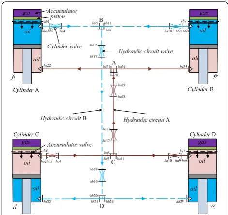
The full mining vehicle studied herein contains two axles that are connected to the vehicle body through leaf spring suspension. A seven-degree-of-freedom (seven-DOF) car model comprising the lumped sprung mass and unsprung mass is used to describe the full mining vehicle. The schematic diagram of a two-axle vehicle with the HIS system is shown in Figure 1. Herein, the sprung mass ms is assumed to be a rigid body with three
directions (zs, θ, and φ). Each unsprung mass mui (i=fr, fl, rr, rl) has a one degree-of-motion freedom in the verti-cal direction (zui). The CG of the vehicle is assumed to be
located on a fixed distance (a and b) from the y-axis and a fixed distance (tf and tr) from the x-axis. The stiffness of
the suspensions is assumed to be equal to ksi, and those
of the tires are assumed to be equal to kti, respectively. zgi
is the excitation of the road surface exerted on the tire. The pitch inertia Iy, and the roll inertia Ix are obtained
about the CG. The subscripts (fr, fl, rr, and rl) are used to denote the front-right, front-left, rear-right, and rear-left, respectively.
Herein, the HIS-equipped vehicle model is a mechani-cal and hydraulic coupled system. The layout for the hydraulic subsystem used in the HIS-equipped vehicle model is shown in Figure 2. The shock absorbers of the CS are replaced by the double acting actuators of the HIS that can directly provide the forces on the vehicle body and wheel assemblies. In the hydraulic subsystem, the hydraulic actuator has a cylinder and a piston, and the cylinder can be divided into a top and a bottom chamber. Furthermore, all the accumulators are integrated into the top chambers. The top chambers include some pin holes, namely accumulator valves, to permit the flow commu-nication between the accumulators and top chambers. These valves can cause the differential pressure in the corresponding chambers. This structure is defined as a pneumatic–hydraulic actuator, which can rapidly allevi-ate the vibration from road excitations. The chambers of actuator assemblies are interconnected by the hydraulic circuits to enable the flow movement among the cham-bers, accumulators, and damper valves.
The wheel assemblies are coupled to each other by the HIS system. In the body bounce motion shown in
Figure 1, the top and bottom chambers are compressed and extended, respectively. Owing to the asymmetry of the hydraulic cylinders, every hydraulic circuit contains a small amount of fluid flowing into the accumulators. This leads to a small pressure change in the two hydrau-lic circuits. Thus, the actuators could generate an addi-tional hydraulic force to restrict the bounce motion of the sprung mass relative to the unsprung mass. In the body pitch motion, all the front and rear suspensions are com-pressed and extended, respectively. The front and rear cylinder bodies move downward and upward relative to the piston rod, respectively. It reduces the volume of the front top and rear bottom chambers, and simultane-ously increases the volume of the front bottom and rear top chambers. Thus, the fluid in circuit B flows into the corresponding accumulator B, and the fluid in the cor-responding accumulator A flows into circuit A. Conse-quently, the pressures in circuits A and B are increased and decreased, respectively. It in return generates the large pitch restoring moment to prevent the vehicle body pitch motion relative to the unsprung mass.
3 Model Development of Vehicles with HIS
Based on the free body diagram method [22] and by regarding the hydraulic forces as external forces, the equations of motion for the integrated mechanical– hydraulic system can be derived as
where M, C, and K are the mass, damping, and stiffness matrices for the mechanical system, respectively. y =
(1)
My¨+Cy˙+Ky=FH +fe,
Figure 1 Schematics of a seven-DOF two-axle vehicle model with HIS system
Hydraulic circuit B Hydraulic circuit A
Cylinder valve
Cylinder A CylinderB
CylinderC Cylinder D
hb2hb3 hb4
hb5 hb11
hb6 hb10hb9hb8
hb12
hb13
hb18
hb19
hb20
hb21
hb22 hb24 hb25
ha2ha3ha4 ha5 ha11
ha6
ha10ha9ha8
ha12
ha13
ha18
ha19
ha20
ha21
ha22 ha24 ha25
fl fr
Accumulator
rl rr
oil gas
gas
oil
oil
oil
oil gas
gas
oil
oil piston
Hydraulic circuit valve
Accumulator valve oil
hb1 hb7
ha1 ha7
B
D A
C
[zsθ φ zufl zufrzurlzurr]T is the displacement vector, fe is
the external force vector. The hydraulic force matrix FH
is defined as FH= D1AcP. The pressure vector P related
to the pressures piT and piB (i= fr, fl, rr, rl) in the
cor-responding cylinder chambers is given as P = [pflT pflB pfrTpfrBprlTprlBprrTprrB]T, the subscript symbols T and B denote the top and bottom chambers, respectively. Ac
= [AflTAflBAfrTAfrBArlTArlBArrTArrB]T is the area matrix
corresponding to the top chamber area AiT and the bot-tom chamber area AiB, respectively. D1 is the linear coef-ficient matrix.
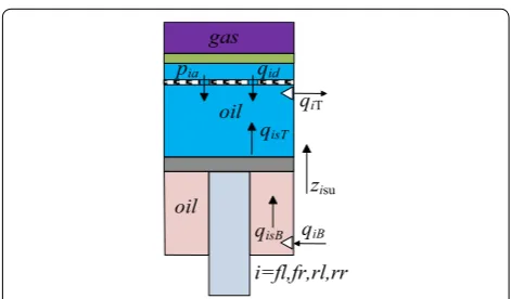
For a double-acting hydraulic actuator, the relative veloc-ity between the cylinder body and the piston rod results in a boundary fluid flow towards the mechanical–fluid interface. The relationship between the relative velocity and fluid flow forms the primary component of the bound-ary flow. Owing to small-amplitude oscillations under low pressure, the compression of the fluid and the cross-line leakage in the cylinder chambers can be ignored. Figure 3 shows the boundary flow conditions for the hydraulic actu-ator model.
In the HIS system, the boundary flow conditions for the double-acting actuators are written as follows:
(2) qflT =qflsT+qfld, qflB=qflsB,
qfrT =qfrsT +qfrd, qfrB=qfrsB,
qrlT=qrlsT+qrld, qrlB=qrlsB,
qrrT =qrrsT+qrrd, qrrB =qrrsB,
where qiT and qiB are the out-flow and in-flow in the cor-responding chambers, respectively. qisT=AiTżisu and qisB
= AiBżisu are volumetric flows generated by the relative
velocity żisu and piston area AiT/AiB in the corresponding
chambers. The pinhole flow qid is assumed to be
propor-tional to the pressure difference between the accumula-tors and top chambers, given by qid= (pia−piT)/ Riav. The
pressure in the corresponding accumulators is defined as pia. The loss coefficient Riav of the accumulator valve
is written as Riav= 128μl0/πdav2 in Ref. [26], where l0 and dav represent the length and diameter of the accumulator
valve, respectively.
As shown, the velocity vector żs-u= [żflsużfrsużrlsużrrsu]T
is relative to the velocity vector ẏ of the lumped sprung mass and unsprung mass, given by żs-u= D2ẏ, where D2 is the linear coefficient matrix. Applying these relation-ships to the four actuator cylinders yields
where the flow vector is Q = [qflTqflBqfrTqfrBqrlTqrlBqrrT qrrB]T, and the accumulator pressure vector Pa = [pfla pfraprla prra]T . Dv1 and Dv2 are the resistance coefficient matrices of the cylinder pressure and accumulator pres-sure, respectively.
To obtain the motion properties of the mechani-cal–fluid coupled system in Eq. (1), the relationship between flow Q and pressure P of the fluid system must be derived. In this study, the transfer impedance matrix method is employed to describe the relationship between the flow rate Q and pressure P, given as Q = TP, where T is the impedance matrix of the hydraulic subsystem determined by the impedance matrices of the fluid com-ponents. As shown in Figure 2, the fluid components primarily include five types of components, namely hydraulic actuators, piston accumulators, three-way junctions, damper valves, and fluid pipelines. For the HIS system, the connection sections of different fluid compo-nents are marked by hai (i= 1, 2,…, 25) and hbi, respec-tively. The state vector composed of the pressure and flow rate (p and q) at the section hji (j=a, b) is defined as xij= [p q]hijT. The transmission matrix Nk is employed
to describe the relationship between state vectors xij and xij+1 of the two terminal sections for the kth component, given as xji+1= Nkxji (k= P,V), where the details of the
transfer matrix Nk for these fluid components can be
found in Ref. [21].
The connectivity matrix N can be obtained by a sequence of multiplications of the involved component impedance matrices according to the theory of transfer matrix. In the hydraulic circuit B of the HIS system, the connectivity matrix N can be written as
(3)
Q=AcD2y˙+Dv1P+Dv2Pa,
oil gas
qiT
qisT
qisB zisu
qiB i=fl,fr,rl,rr oil
qid pia
where the rear subscripts in the matrices above repre-sent the inflow and outflow sections of the correspond-ing components, respectively. The front subscripts P and V refer to the components of fluid pipes and valves, respectively. Accordingly, the relationships between the state vectors at all sections mentioned in Eqs. (4)–(7) are described as
(4)
N11 N12 N21 N22
Nhb2→hb5
=NPhb4→hb5NVhb3→hb4NPhb2→hb3,
(5)
N11 N12 N21 N22
Nhb8→hb11
=NPhb10→hb11NVhb9→hb10NPhb8→hb9,
(6)
N11 N12
N21 N22
Nhb21→hb22
=NPhb21→hb22,
N11 N12
N21 N22
Nhb24→hb25
=NPhb24→hb25,
(7)
N11 N12 N21 N22
Nhb6→hb20
=NPhb19→hb20NVhb18→hb19NPhb13→hb18NVhb12→hb13NPhb6→hb12,
(8)
phb5
qhb5
� �� � xhb5
=Nhb2→hb5
phb2
qhb2
� �� � xhb2
phb11
qhb11
� �� � xhb11
=Nhb8→hb11
phb8
qhb8
� �� � xhb8
phb22
qhb22
� �� � xhb22
=Nhb21→hb22
phb21
qhb21
� �� � xhb21
phb25
qhb25
� �� � xhb25
=Nhb24→hb25
phb24
qhb24
� �� � xhb24
phb20
qhb20
� �� � xhb20
=Nhb6→hb20
phb6
qhb6
� �� � xhb6
The relationships of pressures and flows for the three-way junctions B and D, through applying the continuity equation and assuming no pressure loss, can be defined as follows:
Combining Eqs. (4)–(9), the impedance matrix Tb is
obtained by solving the symbolic equations and given as (9)
qhb5+qhb11=qhb6, phb5=phb6=phb11,
Similarly, the impedance matrix TA of the hydraulic
cir-cuit A can also be obtained. Thus, the impedance matri-ces TA and Tb can be combined and expressed as
where T is the impedance matrix of the HIS system. As shown, the impedance matrix T is determined by the connectivity matrices and related to the precise arrange-ment of the component elearrange-ments in hydraulic circuits.
(10)
qhb2
qhb8
qhb22
qhb25 =
Tb11 Tb12 Tb13 Tb14
Tb21 Tb22 Tb23 Tb24
Tb31 Tb32 Tb33 Tb34
Tb41 Tb42 Tb43 Tb44 � �� � Tb
phb2
phb8
phb22
phb25 . (11) Q=
Tb11 0 Tb12 0 0 Tb13 0 Tb14
0 Ta31 0 Ta32 Ta33 0 Ta34 0 Tb21 0 Tb22 0 0 Tb23 0 Tb24
0 Ta41 0 Ta42 Ta43 0 Ta34 0
0 Ta11 0 Ta12 Ta13 0 Ta14 0
Tb31 0 Tb32 0 0 Tb33 0 Tb34
0 Ta21 0 Ta22 Ta23 0 Ta24 0
Tb41 0 Tb42 0 0 Tb43 0 Tb44
� �� � T P,
Furthermore, Nac is defined as the impedance of the
accumulator. Thus, the accumulator pressure vector can be written as
where qd is the accumulator fluid vector, given as qd=
[qfldqfrdqrldqrrd]T. Owing to the different pressures inside
the accumulators and top chambers generated by the accumulator valves, the fluid-flows qfld, qfrd, qrld, and qrrd
at sections hb1, ha1, hb7, and ha7 are derived as
According to Eq. (13), the relationships between accu-mulator fluid vector qd and pressure vector P can be
rewritten as qd = DvP. Dv is the resistance coefficient
matrix related to the impedance Nac and the loss
coef-ficient Riav. Based on the Laplace transform of Eq. (11)
with zero initial conditions, substituting it into Eq. (3) yields
Combining Eqs. (1) and (14), the equation for the cou-pled system is expressed in the state-space form as
where the system state vector is z = [y ẏ]T and Z(s) is the Laplace transformation of z, F(s) is the Laplace trans-formation of the external force vector fe, A(s) is the
sys-tem characteristic matrix, and B is the input coefficient matrix. They are described in the following form:
(12) Pa= [Nac Nac Nac Nac]TqTd,
(13) qfld=(Nacqfld−phb2)/Rflav, qfrd=(Nacqfrd−phb8)/Rfrav,
qrld=(Nacqrld−pha2)/Rrlav, qrrd=(Nacqrrd−pha8)/Rrrav.
(14) P=s(T−Dv)−1AcD2Y(s).
(15)
sZ(s)=A(s)Z(s)+BF(s),
Frequency dynamic model of a coupled system ( ) ( ) ( ) ( ) s sZ =A Zs s +ΒF s
The identified eigenvalues and eigenvectors
( )
0i s i i i for s
λ= AV =λV J =
Frequency response function matrix H
Power spectral density matrix
T wr
( ) ( )
Xout f = ∗ f
S H S H
Road input vector w
Road spectral matrix Swr
Motion-mode energy method
Free vibration transmissibility and
forced vibration
response analysis Output evaluation indexes
In Eq. (16), Ĉ = C + Ch is the complex damping matrix. Ch = D1Ac(T − Dv)−1AcD2 is the damping contribution from hydraulic subsystem.
4 Vehicle Vibration Characteristics Analysis
The modal analysis process is summarized briefly in the block diagram, as shown in Figure 4. Eq. (15) represents the general equation of motions for the completely cou-pled system in the frequency domain. The frequency response function (FRF) and power spectral density (PSD) response can be derived by the frequency dynamic model of the coupled system to evaluate the vehicle per-formances. Meanwhile, the eigenvalues and eigenvectors are identified to obtain the natural frequency and mode shape of the coupled system. The motion-mode energy method [27] derived by the identified eigenvalues and eigenvectors is employed to analyze the vehicle dynamic characteristics in the frequency domain.
As shown, the system modal characteristic matrix A(s) in Eq. (15) is frequency dependent and this matrix changes with the input frequency s. Based on the defini-tion of the eigenvalue, soludefini-tions of the equadefini-tion |det(A(s) −sI)| = 0 are the eigenvalues of A(s). Owing to the large numerical values of some of the parameters, the exact eigenvalues of A(s) are difficult to obtain by numerical means. Thus, the approximate roots are acceptable if the function J(s) = |det(A(s) −sI)| is approaching a local minimum value in the vicinity of s. To obtain the modal parameters, the Matlab optimization library function fminsearh was used to identify the real eigenvalues and eigenvectors according to the local minimum values.
Using the optimization method, the complex eigenval-ues λi and eigenvectors Vi resulting from the solutions of
the equation |det(A(s) −sI)| = 0 are given as
where the first seven terms of Vi (i= 1, 2,…, 7)
repre-sent the mode shape of the displacement vector. For (16) A(s)=
O I
−M−1K −M−1C(s)ˆ
, B=
O
M−1
.
(17) i=s, AVi =iVi, for J(s)=0,
each complex root λi = ai + jbi, the natural frequency fi and damping ratio ξi for each mode are given as fi=sqrt(a2i+b2i)/2π and ξi=ai/sqrt(ai2+bi2).
The modal transition matrix can be determined by the eigenvalue matrix and eigenvector matrix, and it can be defined as
where ψ = diag[λ1 λ2 λ3 λ4 λ5 λ6 λ7] is the eigenvalue matrix and Λ = [V1 V2 V3 V4 V5 V6 V7] is the eigenvector matrix.
The system state vector Z can be described as a super-position of the motion-modes through modal transfor-mation as
where u = [u1u2 u3u4 u5u6u7]T is a modal amplitude vector. As shown, the modal amplitude ui is a complex
number that contains both a scalar quantity and the phase information of this mode in the frequency domain.
As L is a known matrix determined by the coupled mechanical–hydraulic system, the modal amplitude vec-tor u(f) can be obtained by applying the least-squares method, and the form of u is written as
Subsequently, the modal amplitude vector u must be transferred into a physical coordinate as [di ḋi], where di = real(uiVi), ḋi = real(uiViλi), and di can be written
as di = [dmi dui] referring to the displacement vector y
defined in Eq. (1). In this study, dmi and dui are used to
describe the body and wheel motions, respectively. The vector [di ḋi] is the corresponding state vector
compo-nent in the form of the displacement and velocity, and represents the ith motion-mode’s contribution to the vehicle’s body and wheel motions. The energy in one motion-mode does not exchange with the others accord-ing to the orthogonal property of modal transformation, and its energy is continuously converted between the potential energy and kinetic energy, and decays owing to the damping effect. The kinetic energy eki, potential
energy epi, and the sum of mechanical energy ei for each
motion-mode stored in the ith mode can be given as (18)
L= [� ΛΨ]T14×7,
(19) Z =Lu(f),
(20)
u(f)=(LTL)−1LTZ.
(21) eki= 1
2
˙
dTiMd˙i, epi=
1
2
D3dmi−dui
dui−dgi
T
Dk
D3dmi−dui
dui−dgi
,
where Dk= diag[ksflksfrksrlksrr]T and dgi is the projection
of the road input in the same coordinate frame with the vehicle motion-mode, which can be determined by the same principle of modal transformation. D3 is the coef-ficient matrix related to the physical parameters of the vehicle model.
In this study, the FRF is employed to analyze the vibra-tion characteristics of the suspension system in the fre-quency domain. The suspension vibration performances can be evaluated using the displacement response ampli-tude transmissibility between the displacement vector y and road input vector w = [0 0 0 zgflzgfrzgrlzgrl]T.
Com-bining Eqs. (1) and (20), the FRF matrix Hdis from the
road input vector w to the displacement output vector y is described as
where s = j2πf and W(s) is the Laplace transformation of the road input vector w, and β(s) is a 7 × 7 input coef-ficient matrix, given as β(s) = diag[0 0 0 ktflktfrktrlktrr].
The FRF matrix is used to describe the system displace-ment response to any harmonic road excitation in the frequency domain.
To evaluate ride comfort, the corresponding trans-fer functions of the vibration accelerations, suspension deflections, and tire dynamic forces, which are related to the road input vector W(s), are defined as follows, respectively:
where the Laplace transformations of the vibration accelerations, suspension deflections, and tire dynamic forces can be defined as Xacc=s2Y(s), Xsus= D2Y(s), and Xtire= β(s)(Y(s) − W(s)), respectively.
To obtain the evaluation outputs Xout= [Xacc Xsus Xtire]T, the entities of all transfer functions are
assem-bled as follows:
(22) Hdis(s)=
Y(s)
W(s) =(s
2
M+sCˆ(s)+K)−1β7×7(s),
(23)
Hacc=
s2Y(s)
W(s) =s
2 Hdis,
Hsus =
D2Y(s)
W(s) =D2Hdis,
Htire=
β(s)(Y(s)−W(s))
W(s) =β(s)(Hdis−I),
where Wr(s) is the Laplace transformation of the reduced
road displacement vector wr = [zgfl zgfrzgrl zgrl]T, DT is
the transfer coefficient matrix that can describe the cor-responding relationship between the reduced road dis-placement vector wr and the road input vector w, given as w = DTwr, and H is defined as the transfer function from
inputs Wr(s) to the evaluation outputs.
The PSD matrix SXout(f) can be derived from the
com-plex transfer function, and the detailed expression is defined as
where H* and HT are the complex conjugate matrix and transpose matrix, respectively. Swr(f) is the spectral
den-sity matrix at four tire–road contact points, given by
where l is the wheel base, and v is the vehicle velocity. Sd
and Sr are the auto-spectral density and cross-spectral (24)
Xacc
Xsus
Xtire
� �� �
Xout =
Hacc
Hsus
Htire
W(s)=
Hacc
Hsus
Htire
DT
� �� �
H
Wr(s),
(25) SXout(f)=H∗Swr(f)HT,
(26) Swr(f)=
Sd Sr Sde−j2πfl/v Sre−j2πfl/v Sr Sd Sre−j2πfl/v Sde−j2πfl/v Sdej2πfl/v Srej2πfl/v Sd Sr Srej2πfl/v Sdej2πfl/v Sr Sd
Table 1 Physical parameters of a seven‑DOF vehicle model
Parameter Value
density functions of the road surface model, respectively. They can be described as in Ref. [24]:
where n=f/v is the spatial frequency, n0 is the reference spatial frequency (n0= 0.1), Sd(n0) is the spatial PSD at the reference spatial frequency, ҡ= 2 is the undulation exponent, and B is the wheel track. The symbols Ga and Be are defined as Gamma and Bessel functions, respec-tively. The diagonal elements of SXout(f) represent the
direct spectral densities of the output variable Xout.
5 Numerical Results and Discussions
The performance comparisons of mining vehicles with the CS and HIS systems are presented in this section. For the mining vehicle with the CS system, the stiffness (27)
Sd(n)=Sd(n0)(
n n0
)−κ,
Sr(n)=
2nκ
0Sd(n0)(πB/n)κ/2
Ga(κ/2)
Be(2πBn),
of mechanical suspensions kpsj (j=fr, fl, rr, rl) is designed
to be stiff to increase the pitch mode stiffness. However, the stiff suspension can cause poor ride comfort. Thus, The CS system cannot well coordinate bounce with the pitch vibrations of the mining vehicles. For the mining vehicle with the HIS system, the stiffness of the mechani-cal suspensions kbsj can be designed to be soft, which is
smaller than kpsj, and the hydraulic subsystem can
pro-vide additional pitch mode stiffness. For the simplifica-tion, the vehicle model with CS (equivalent stiffness kpsj)
and HIS are defined as VCS-EP and VHIS, respectively. The dynamic performance of the roll motion is not the research emphasis in this study owing to the low velocity of the mining vehicles not exceeding 50 km/h. The basic physical parameters of a seven-DOF vehicle model are given in Table 1. Table 2 lists the hydraulic parameters of the HIS system.
5.1 Dynamic Performance Evaluation
The identified natural frequencies, damping ratios, and corresponding mode shapes of VCS-EP and VHIS are presented in Table 5. As shown in Table 5, vehicle body– wheel motion-modes referring to the relative motion between body and wheels can be classified into seven modes in terms of the modal shapes. The normalized factor of the state vectors is used to distinguish seven modes. The motion corresponding to the maximum absolute value of the normalized factor in each modal shape represents one mode of the body-wheel motions. The values in the black bold font reveal that the first three mode shapes are called the body-dominated motion-modes, namely roll (1st), bounce (2nd), and pitch (3rd) motions of the sprung mass, and the following four mode shapes are called the wheel-dominated motion-modes, namely, the pitch (4th), bounce (5th), roll (6th), and warp (7th) motions of the unsprung mass. For the VCS-EP, the equivalent stiffness kpsj (j=fl, fr, rl, rr) is 265 N/mm. For
Table 2 Hydraulic system parameters
Parameter Value
Hydraulic fluid density (kg/m3) 870
Bulk modulus (MPa) 1400
Accumulator pre-charge gas volume (L) 0.25 Accumulator pre-charge pressure (bar) 10 Diameter of cylinder piston (m) 0.05 Diameter of cylinder piston rod (m) 0.036 Mean system pressure P0 (bar) 23 Loss coefficient of cylinder valve RCV (GPa∙s/m3) 1.5 Loss coefficient of hydraulic circuit valve RHCV (GPa∙s/m3) 0.8 Loss coefficient of accumulator valve RAV (GPa∙s/m3) 1.5
100 101
10-2 10-1 100 101
Frequency (Hz)
Ve
rtic
al
di
sp
la
cem
ent
ga
in
(m
/m
)
VCS-EP VHIS
100 101
10-2 10-1 100 101
Frequency (Hz)
Pi
tc
h
ang
le
ga
in
(ra
d/
m)
VCS-EP VHIS
the VHIS, the equivalent stiffness kbsi (i=fl, fr) and kbsj
(j=rl, rr) are 129.2 N/mm and 167.4 N/mm, respectively. In Table 5, the HIS system can effectively increase the pitch mode (the 3rd mode) frequency (from 2.539 Hz/ VCS-EP to 2.747 Hz/VHIS) of the sprung mass vibration, and reduce the bounce mode (the 2nd mode) frequency
(from 2.351 Hz/VCS-EP to 1.906 Hz/VHIS). The result illustrates that the proposed HIS system can provide a higher pitch mode stiffness owing to the large fluids rap-idly flowing into the accumulator in the pitch mode, and the lower bounce mode stiffness owing to the large flu-ids freely flowing in the hydraulic circuits. Owing to the
100 101
10-4 10-2 100
Frequency (Hz)
Suspensi
on
de
flec
tion
ga
in
(m
/m
)
Front suspension@VCS-EP Front suspension@VHIS Rear suspension@VCS-EP Rear suspension@VHIS
100 101
102 103 104 105 106 107
Frequency (Hz)
Ti
re
dynam
ic
fo
rc
e
gai
n
(N
/m
)
Front tire@VCS-EP Front tire@VHIS Rear tire@VCS-EP Rear tire@VHIS
Figure 6 Suspension deflections and tire dynamic forces under front wheel input
100 101
10-2 10-1 100 101
Frequency (Hz)
Ve
rtic
al
di
sp
la
ce
me
nt
ga
in
(m
/m
)
VCS-EP VHIS
100 101
10-2 10-1 100 101
Frequency (Hz)
Pi
tc
h
angl
e
gai
n
(rad/
m)
VCS-EP VHIS
Figure 7 CG’s bounce displacement and pitch angle under rear wheel input
100 101
10-4 10-2 100
Suspensi
on
de
flec
tion
ga
in
(m
/m
)
Frequency (Hz) Front suspension@VCS-EP Front suspension@VHIS Rear suspension@VCS-EP Rear suspension@VHIS
100 101
102 103 104 105 106 107
Frequency (Hz)
Ti
re
dyna
mi
c
fo
rc
e
ga
in
(N
/m
)
Front tire@VCS-EP Front tire@VHIS Rear tire@VCS-EP Rear tire@VHIS
soft mechanical suspensions, the body roll mode (the 1st mode) frequencies (1.286 Hz/VHIS) of the VHIS are lower than that of the VCS-EP. It is also observed that the proposed HIS system is unable to provide the extra roll mode stiffness.
Additionally, the HIS system can reduce the natural fre-quencies of the wheel-dominated motion-modes, involv-ing the wheel pitch mode (the 4th mode in VHIS, 9.158 Hz), wheel bounce mode (the 5th mode in VHIS, 10.419 Hz), wheel roll mode (the 6th mode in VHIS, 11.226 Hz), and wheel warp mode (the 7th mode in VHIS, 12.530 Hz). In the previous study [23], it can be seen that the lower warp mode stiffness can improve the ground hold-ing performance. From the comparisons of the mode shapes, the HIS system can decouple the body bounce and pitch modes, and intensify the coupling of wheel bounce and pitch modes, which is beneficial to balance the distribution of the front and rear tire forces. Further-more, it is observed that the HIS system can increase the damping ratios corresponding to both the body modes (roll, bounce, and pitch) and wheel modes (bounce and pitch) of the integrated system, and the high damping can eliminate transient oscillations.
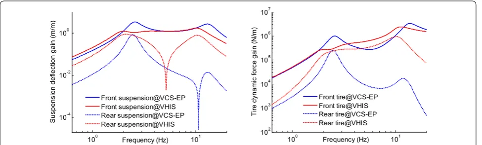
According to the FRF matrix Hdis defined by Eqs. (27) and (28), the bilogarithmic graphs of the frequency response of CG’s bounce displacement, pitch angle, suspension deflections, and tire dynamic forces for the VCS-EP and VHIS under the front wheel input (w = [0 0 0 zgflzgfr 0 0]T) and rear wheel input (w = [0 0 0 0 0 zgrl zgrr]T) are plotted in Figures 5, 6, 7 and 8, respectively.
It shows that the HIS system reduces the peak vibration frequency for the bounce mode and increases the peak vibration frequency for the pitch mode. Under the front and rear wheel inputs, the peak values of the frequency response for the VHIS in the bounce and pitch modes are smaller than those of the VCS-EP. For the bounce mode, the transmissibility of the VHIS is suppressed if
the frequency is less than 8 Hz. For the pitch mode, the frequency response of the VHIS located before and after the natural vibration frequency is slightly suppressed and enlarged, respectively.
As shown in Figures 6 and 8, the peak values of the front suspension deflections and front tire dynamic forces are reduced by the HIS under the front wheel input. For the front suspension deflections of the VHIS, the frequency response lower than the natural vibration frequency is slightly enlarged, and that higher than the natural vibration frequency is unchanged; further, the HIS system reduces the transmissibility in high frequency ranges. For the front tire dynamic forces, the proposed HIS system maintains the same transmissibility located before the oscillation frequency, but slightly increases the transmissibility higher than the natural vibration fre-quency, and the frequency response is reduced in higher frequency ranges. Moreover, the frequency responses of the rear suspension deflections and rear tire dynamic forces under the left wheel input for the VHIS are much larger than those of the VCS-EP. This phenomenon illus-trates that a mining vehicle with the HIS system trans-mits a greater degree of motion to the opposite wheels under the corresponding mode vibration. As shown, the frequency responses of the VHIS exhibit much broader peak ranges than the VCS-EP owing to the interconnec-tion mechanism. For the VHIS, the addiinterconnec-tional excitainterconnec-tion applied to the front or rear wheels can be transmitted much more efficiently to the opposite wheel through the hydraulic system. This result is helpful to balance the dynamic forces between the front and rear wheels, thus enhancing the ground holding performance.
The frequency responses of the bounce and pitch modes motion-energy for the VCS-EP and VHIS under the front and rear wheel inputs are shown in Figure 9. The transmissibility of the bounce mode motion-energy is reduced by the HIS system, but the frequency response
100 101
103 104 105 106 107
Frequency (Hz)
Mo
da
l ener
gy
ga
in
(J
/m
)
Bounce mode@VCS-EP Bounce mode@VHIS Pitch mode@VCS-EP Pitch mode@VHIS under front
wheel input
100 101
103 104 105 106 107
Frequency (Hz)
Mo
da
l ener
gy
ga
in
(J
/m
)
Bounce mode@VCS-EP Bounce mode@VHIS Pitch mode@VCS-EP Pitch mode@VHIS under rear
wheel input
of the pitch mode motion-energy is enlarged. Based on the mode motion-energy definition, the complex eigen-values exhibit a significant effect on the mode motion-energy. From Table 5, the modulus of the bounce mode
eigenvalue for the VHIS is smaller than that of the VCS-EP, but the value of the pitch mode eigenvalue is larger than that of the VCS-EP. This is clearly a reflec-tion that the vehicle with a softer bounce mode stiffness has a lower bounce mode motion-energy, and that with a stiffer pitch mode stiffness has a higher pitch mode motion-energy. Thus, these results show that the pro-posed HIS system can reduce the bounce mode stiffness and increase the pitch mode stiffness.
To evaluate the vehicle dynamic performances, the road surface spectrums including two types of the ran-dom road model (medium-smooth and rough roads) are applied in the simulation. Based on the road model description in Ref. [28], Sd(n0) = 0.64 × 10⁶ and
10.64 × 10⁶ are used to describe these two average road types. The comparisons of PSD responses for the VCS-EP and VHIS with different speeds (20, 30, 40, and 50 km/h) are presented to investigate the suspension proper-ties. The frequency-weighted root mean square (RMS) bounce, pitch angular and roll angular accelerations of the vehicle body are used to quantify the ride comfort
100 101
10-15 10-10 10-5
Frequency (Hz)
Pi
tc
h
angl
e
PSD
(ra
d
2 /H
z)
20 km/h@VCS-EP 20 km/h@VHIS 30 km/h@VCS-EP 30 km/h@VHIS 40 km/h@VCS-EP 40 km/h@VHIS 50 km/h@VCS-EP 50 km/h@VHIS
11.2-14.1 Hz
17.8-22.4 Hz 4.47-5.62 Hz
2.82-3.55 Hz
28.2-35.5 Hz 1.12-1.41 Hz
1.78-2.24 Hz
7.08-8.91 Hz
0.71-0.89 Hz
Figure 10 Pitch angle response in one-third octave bands under rough road
100 101
10-10 10-8 10-6 10-4 10-2
Frequency (Hz)
Fr
on
t suspensi
on
PSD
(m
2/H
z)
20 km/h@VCS-EP 20 km/h@VHIS 30 km/h@VCS-EP 30 km/h@VHIS 40 km/h@VCS-EP 40 km/h@VHIS 50 km/h@VCS-EP 50 km/h@VHIS
100 101
100 102 104 106 108
Frequency (Hz)
Fr
on
t tire
dyna
mi
c
fo
rc
e
PSD
(N
2/H
z)
20 km/h@VCS-EP 20 km/h@VHIS 30 km/h@VCS-EP 30 km/h@VHIS 40 km/h@VCS-EP 40 km/h@VHIS 50 km/h@VCS-EP 50 km/h@VHIS
Figure 11 Front suspension deflection and tire dynamic force under rough road
100 101
10-10 10-8 10-6 10-4 10-2
Frequency (Hz)
Rear
suspensi
on
PSD
(m
2/H
z)
20 km/h@VCS-EP 20 km/h@VHIS 30 km/h@VCS-EP 30 km/h@VHIS 40 km/h@VCS-EP 40 km/h@VHIS 50 km/h@VCS-EP 50 km/h@VHIS
100 101
100 102 104 106 108
Frequency (Hz)
R
ear
tire
dyna
mi
c
fo
rc
e
PSD
(N
2/H
z)
20 km/h@VCS-EP 20 km/h@VHIS 30 km/h@VCS-EP 30 km/h@VHIS 40 km/h@VCS-EP 40 km/h@VHIS 50 km/h@VCS-EP 50 km/h@VHIS
according to ISO-2631-1 [29], and they can be written as follows:
where χb, χp, and χr are the weighting factors of
the bounce, pitch, and roll modes, respectively; SXout11, SXout22, and SXout33 are the PSD responses of the CG’s vertical, pitch, and roll angular accelerations, respectively.
Figure 10 shows the pitch angular response in one-third octave bands for the VCS-EP and VHIS under the rough road. The HIS system can effectively reduce the pitch angle of the vehicle body in a low frequency range, and maintain the pitch angle response in the range of 11.2– 14.1 Hz, but slightly increase the frequency response in high frequency ranges. This is owing to the higher pitch stiffness provided by the HIS system. The PSD responses of the suspension deflections and tire dynamic forces for the VCS-EP and VHIS under the rough road are shown in Figures 11 and 12. The frequency responses of the sus-pension deflections and tire dynamic forces are reduced by the HIS system in low frequency ranges, and those in high frequency ranges are unchanged. The first natural vibration frequency of the PSD response is reduced for the VHIS with different speeds from 20 to 50 km/h owing to the lower roll stiffness. The PSD response peak values of the suspension deflections and tire dynamic forces for the VHIS are evidently smaller than those of the VCS-EP. These results show that the HIS system can reduce the suspension deflections and tire dynamic forces to improve the holding ground performance, and decrease the bounce and pitch angular accelerations to improve the ride comfort for the mining vehicle.
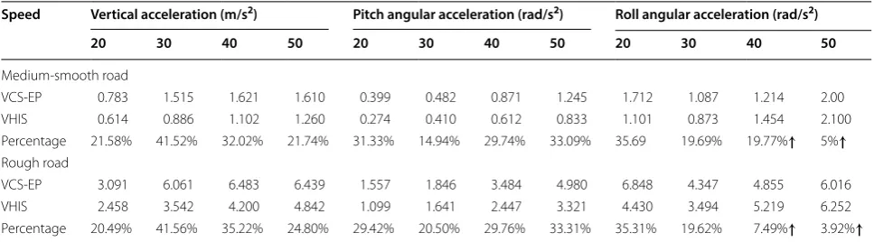
The RMS acceleration comparisons of the bounce, pitch, and roll modes between the VHIS and VCS are shown in Table 3. It shows that the proposed HIS can suppress the bounce and pitch motions of the (28)
ai=
χi2(f)SXoutjj(f), i=b,p,r jj=11, 22, 33,
vehicle body. The RMS vertical accelerations under the medium-smooth road with different speeds have been decreased from 0.783 to 0.614 m/s2, 1.515 to 0.886 m/ s2, 1.621 to 1.102 m/s2, and 1.610 to 1.260 m/s2. The HIS system has significantly reduced the RMS vertical accelerations under the rough road by 20.49%, 41.56%, 35.22%, and 24.80%, respectively. Meanwhile, the RMS pitch angular accelerations under medium-smooth and rough roads have been decreased by no less than 14.5% and 20%, respectively. The RMS roll angu-lar accelerations at low speeds (20 and 30 km/h) are almost reduced by 35% and 20%, respectively. And the HIS system has slightly increased the RMS roll angular accelerations at high speeds (40 and 50 km/h) within an accepted variance. These results demonstrate that the proposed HIS system can improve the mining vehicle ride comfort.
5.2 Parametric Sensitivity Analysis
To further illustrate the decoupled advantages of the proposed HIS, the parametric sensitivity analysis of the damper valves is presented in this section, includ-ing the cylinder valve (CV), hydraulic circuit valve (HCV), and accumulator valve (AV). These parameters are employed to analyze their effects on the vibration transmissibility of the vehicle body bounce, pitch, and roll modes. Figure 12 shows the frequency responses of the CG’s bounce displacement, pitch angle, and roll angle with different loss coefficients for the VHIS under the front-left wheel input w = [0 0 0 zgfl 0 0 0]T.
The front-left wheel input can easily induce the body bounce, pitch, and roll modes. From Figure 13(a), the CV provides the higher roll mode damping than the bounce mode damping, and has little influence on the pitch mode damping. Further, it is observed that the higher CV loss coefficient leads to a stiffer roll mode. From Figure 13(b), the HCV appears to generate a Table 3 RMS acceleration comparisons
Speed Vertical acceleration (m/s2) Pitch angular acceleration (rad/s2) Roll angular acceleration (rad/s2)
20 30 40 50 20 30 40 50 20 30 40 50
Medium-smooth road
VCS-EP 0.783 1.515 1.621 1.610 0.399 0.482 0.871 1.245 1.712 1.087 1.214 2.00 VHIS 0.614 0.886 1.102 1.260 0.274 0.410 0.612 0.833 1.101 0.873 1.454 2.100 Percentage 21.58% 41.52% 32.02% 21.74% 31.33% 14.94% 29.74% 33.09% 35.69 19.69% 19.77%↑ 5%↑ Rough road
significant effect on the bounce mode characteristic. However, it is nearly unrelated to the dynamic charac-teristics of the roll mode. From Figure 13(c), the AV is primarily designed to control the pitch mode property. The comparisons of natural frequency and damping ratio with the CV, HCV and AV loss coefficients are
presented in Table 4. These results are in accord with the above phenomena, and prove that the proposed HIS system can decouple the vehicle body modes by adjusting the corresponding loss coefficient, which is the irreconcilable contradiction for the CS system.
5 10 15
0 0.5 1 1.5 2 2.5
Frequency (Hz)
Amp
lit
ude
ga
in
(m
/s
2/m
, ra
d/
s
2/m
)
1 2 3
0.2 0.4
0.6 1.6e98e8
4e8
2 3 4
0.2 0.3
0.5 1 1.5 2
1 2 roll mode
bounce mode pitch mode
b
5 10 15
0 0.5 1 1.5 2 2.5
Frequency (Hz)
Amp
lit
ude
ga
in
(m
/s
2 /m
or
ra
d/
s
2 /m
)
1 2 3
0.2 0.4 0.6
2.5e9 1.5e9 1e9
1 1.2 1.4
1 2 3
2 4 6
0.2 0.3 0.4 bounce mode
pitch mode
roll mode c
0 5 10 15
0 0.5 1 1.5 2 2.5 3
Frequency (Hz)
Amp
lit
ude
ga
in
(m
/s
2/m
or
rad/
s
2/m
)
2.5e9 1.5e9 1e9 0.8 1 1.2 1.4 1.6 1
2 3
1 2 3
0.2 0.4 0.6
2 3 4
0.2 0.250.3 bounce mode roll mode
pitch mode
a
Figure 13 Vibration transmissibility with different loss coefficients: (a) CV, (b) HCV, (c) AV
Table 4 Comparisons of natural frequency and damping ratio
RCV (GPa∙s/m3) RHCV (GPa∙s/m3) RAV (GPa∙s/m3)
1 1.5 2.5 0.4 0.8 1.6 0.1 1.5 2.5
Roll mode
fd (Hz) 1.264 1.286 1.329 1.286 1.286 1.286 1.296 1.286 1.271
ξ 0.077 0.097 0.117 0.097 0.097 0.097 0.097 0.097 0.099 Bounce mode
fd (Hz) 1.909 1.907 1.902 1.9125 1.907 1.890 1.909 1.907 1.901
ξ 0.190 0.205 0.235 0.159 0.205 0.300 0.190 0.205 0.237 Pitch mode
6 Conclusions and Future Work
A new HIS system to was proposed herein to improve the bounce and pitch motion performances for a min-ing vehicle. The integrated dynamic equations of the mechanical–hydraulic coupled system were derived using the impedance transfer matrix and free-body dia-gram methods. Based on the derived equations, the modal analysis method was employed to obtain the free vibration transmissibilities and force vibration responses under different road excitations. The dynamic character-istic comparisons between the VCS-EP and VHIS were presented to verify the prominent advantages of the HIS system. These results illustrated that the proposed HIS system could decouple the bounce and pitch modes, and intensify the coupling of wheel bounce and pitch modes to balance the distribution of tire dynamic forces. Fur-thermore, the HIS system could provide additional pitch stiffness to control the vehicle pitch motion, reduce the bounce stiffness to improve ride comfort, and increase the corresponding mode damping to eliminate transient oscillations in the lower frequency range.
Herein, the most obvious limitation is that the HIS sys-tem could not provide adequate roll stiffness to control the roll mode. Another limitation was that the modal analysis method was linear in this study. However, the suspension system and tire assembly often exhibit many nonlinearities for practical applications. Thus, the per-formances of the bounce, pitch, and roll modes would be considered for the passive HIS system, and the extension of the proposed methodology to a full nonlinear vehicle model must be explored in the future. Additionally, the semi-active or active control strategy for the HIS system must be considered as future works to improve the ride comfort and handling performance of the mining vehicle based on control theories.
Authors’ Contributions
JZ and YD was in charge of the whole trial; JZ wrote the manuscript; NZ, BZ, HQ and MZ assisted with sampling and laboratory analyses. All authors read and approved the final manuscript.
Author Details
1 State Key Laboratory of Advanced Design and Manufacturing for Vehicle
Body, College of Mechanical and Vehicle Engineering, Hunan University, Table 5 The comparisons of natural frequency and mode shape
Mode shape
1st 2nd 3rd 4th 5th 6th 7th
Description Body-dominated
roll mode Body-dominated bounce mode Body-dominated pitch mode Wheel-dominated pitch mode Wheel-domi-nated bounce mode
Wheel-domi-nated roll mode Wheel-dominated warp mode VCS-EP
s − 0.72 + 9.83i − 1.62 + 14.77i − 1.90 + 15.95i − 10.27 + 73.51i − 13.17 + 83.50i − 9.64 + 73.69i − 12.32 + 83.83i
fd (Hz) 1.564 2.351 2.539 11.699 13.286 11.728 13.342
ξ 0.073 0.109 0.118 0.138 0.156 0.129 0.145
zs 0 1 − 0.525 − 0.005i − 0.029 − 0.030i − 0.023 − 0.026i 0 0
θ 0 0.240 + 0.002i 1 − 0.020 − 0.021i 0.017 + 0.020i 0 0
φ 1 0 0 0 0 − 0.037 − 0.036i 0.019 + 0.022i
zufl 0.059 + 0.009i 0.114 + 0.026i − 0.406 − 0.104i − 0.003 + 0.007i 1 0.000 − 0.021i − 1 zufr − 0.059 − 0.009i 0.114 + 0.026i − 0.406 − 0.104i − 0.003 + 0.007i 1 − 0.000 + 0.021i 1
zurl 0.086 + 0.013i 0.257 + 0.061i 0.184 + 0.046i 1 0.001 − 0.005i 1 0.001 − 0.014i zurr − 0.086 − 0.013i 0.257 + 0.061i 0.184 + 0.046i 1 0.001 − 0.005i − 1 − 0.001 + 0.014i VHIS
s − 0.81 + 8.08i − 2.40 + 12.00i − 6.79 + 17.18i − 32.02 + 57.63i − 11.97 + 65.45i − 6.01 + 70.55i − 7.99 + 78.71i
fd (Hz) 1.286 1.906 2.747 9.158 10.419 11.226 12.530
ξ 0.097 0.205 0.358 0.488 0.179 0.087 0.099
zs 0 1 0.001 − 0.097i − 0.002 − 0.083i 0.030 − 0.087i 0 0
θ 0 − 0.013 + 0.036i 1 0.043 + 0.166i − 0.032 − 0.004i 0 0
φ 1 0 0 0 0 0.020 + 0.027i 0.007 + 0.017i
zufl 0.034 + 0.008i 0.114 + 0.045i − 0.273 − 0.305i − 0.833 − 0.187i 0.945 + 0.263i − 0.004 + 0.009i − 1 zufr − 0.034 − 0.008i 0.114 + 0.045i − 0.273 − 0.305i − 0.833 − 0.187i 0.945 + 0.263i 0.004 − 0.009i 1
Changsha 410082, China. 2 Automotive Research Institute, Hefei University
of Technology, Hefei 230009, China. 3 School of Automotive and
Transporta-tion Engineering, Hefei University of Technology, Hefei 230009, China.
Authors’ Information
Jie Zhang, born in 1987, is currently a PhD candidate at State Key Laboratory of Advanced Design and Manufacture for Vehicle Body, Hunan University, China. He received his bachelor degree from Yangtze University, China, in 2011. His research interests include control, modeling, and estimation of driver-vehicle system dynamics.
Yuanwang Deng, born in 1968, is currently an associate professor at Col-lege of Mechanical and Vehicle Engineering, Hunan University, China. He received his PhD degree from Huazhong University of Science and Technology, China, in 2002. His research interests include heat transfer theory, engine electronic control technology and mechanical system dynamics.
Nong Zhang, born in 1959, is currently a professor at Automotive Research Institute, Hefei University of Technology, China. He received his PhD degree from University of Tokyo, Japan, in 1989. His current research interests include dynamics and control of automotive systems.
Bangji Zhang, born in 1967, is currently a professor at State Key Laboratory of Advanced Manufacture and Design for Vehicle Body, Hunan University, China.
Hengmin Qi, born in 1990, is currently a PhD candidate at State Key Labora-tory of Advanced Design and Manufacture for Vehicle Body, Hunan University, China. He received his bachelor’s degree from China University of Petroleum, China, in 2012. His research interests include design and analysis of hydrauli-cally interconnected suspension system and vehicle system dynamics.
Minyi Zheng, born in 1983, is currently a lecturer at School of Automo-tive and Transportation Engineering, Hefei University of Technology, China. He received his Ph.D. from Hunan University, China, in 2016 His research interests include vehicle dynamics and parameter identification.
Acknowledgements
The authors sincerely thanks to Assistant Professor Fei Ding of Hunan Univer-sity for his critical discussion and reading during manuscript preparation.
Competing Interests
The authors declare no competing financial interests.
Funding
Supported by National Natural Science Foundation of China (Grant Nos. 51805155, 51675152), Foundation for Innovative Research Groups of National Natural Science Foundation of China (Grant No. 51621004), and Open Fund in the State Key Laboratory of Advanced Design and Manufacture for Vehicle Body (Grant No. 71575005).
Appendix
Table 5 shows the comparisons of natural frequency and mode shape between the VCS-EP and VHIS.
Publisher’s Note
Springer Nature remains neutral with regard to jurisdictional claims in pub-lished maps and institutional affiliations.
Received: 27 March 2017 Accepted: 8 January 2019
References
[1] T Eger, J Stevenson, P É Boileau, et al. Predictions of health risks associated with the operation of load-haul-dump mining vehicles: Part 1—Analysis of whole-body vibration exposure using ISO 2631-1 and ISO-2631-5 standards. International Journal of Industrial Ergonomics, 2008, 38(9-10): 726-738.
[2] D P Cao, X B Song, M Ahmadian. Editors’ perspectives: road vehicle suspension design, dynamics, and control. Vehicle System Dynamics, 2001, 49(1-2): 3–28.
[3] M C Smith, F C Wang. Controller parameterization for disturbance response decoupling: application to vehicle active suspension control.
IEEE Transactions on Control Systems Technology, 2002, 10(3): 393-407. [4] H Y Li, H H Liu, H J Gao, et al. Reliable fuzzy control for active suspension
systems with actuator delay and fault. IEEE Transactions on Fuzzy Systems, 2012, 20(2): 342-357.
[5] S Y Han, C H Zhang, G Y Tang. Approximation optimal vibration for networked nonlinear vehicle active suspension with actuator time delay.
Asian Journal of Control, 2017, 19(3): 983-995.
[6] W C Sun, H H Pan, H J Gao. Filter-based adaptive vibration control for active vehicle suspensions with electrohydraulic actuators. IEEE Transac-tions on Vehicular Technology, 2016, 65(6): 4619-4626.
[7] S Bououden, M. Chadli, H R Karimi. A robust predictive control design for nonlinear active suspension systems. Asian Journal of Control, 2016, 18(1): 122-132.
[8] Y B Huang, J Na, X Wu, et al. Adaptive control of nonlinear uncertain active suspension systems with prescribed performance. ISA Transactions, 2015, 54(1): 145-155.
[9] X J Wu, B Zhou, G L Wen, et al. Intervention criterion and control research for active front steering with consideration of road adhesion. Vehicle System Dynamics, 2018, 56 (4): 553-578.
[10] J Wu, S Chen, B H Liu, et al. A human-machine-cooperative-driving con-troller based on AFS and DYC for vehicle dynamic stability. Energies, 2017, 10(11): 17-37.
[11] S Chen, L Li, J Chen. Fusion algorithm design based on adaptive SCKF and integral correction for side-slip angle observation. IEEE Transactions on Industrial Electronics, 2018, 65(7): 5754-5763.
[12] J Zhao, P K Wong, X B Ma, et al. Chassis integrated control for active suspension, active front steering and direct yaw moment systems using hierarchical strategy. Vehicle System Dynamics, 2017, 55(1): 72-103. [13] A M C Odhams, D Ceon. An analysis of ride coupling in automobile
suspensions. Proceedings of the Institution of Mechanical Engineers, Part D: Journal of Automobile Engineering, 2006, 220(8): 1041-1061.
[14] M C Smith, G W Walker. Interconnected vehicle suspension. Proceedings of the Institution of Mechanical Engineers, Part D: Journal of Automobile Engineering, 2005, 219(3): 295-307.
[15] Z X Li, L Y Ju, H Jiang, et al. Experimental and simulation study on the vibration isolation and torsion elimination performances of intercon-nected air suspensions. Proceedings of the Institution of Mechanical Engineers, Part D: Journal of Automobile Engineering, 2016, 230(5): 679-691. [16] N Mace. Analysis and synthesis of passive interconnected vehicle suspensions.
Cambridge: University of Cambridge, 2004.
[17] D P Cao, S Rakheja, C Y Su. Dynamic analyses of roll plane interconnected hydro-pneumatic suspension systems. International Journal of Vehicle Design, 2008, 47(1): 51-80.
[18] S Bhave. Effect of connecting the front and rear air suspensions of a vehicle on the transmissibility of road undulation inputs. Vehicle System Dynamics, 1992, 21(1): 225-245.
[19] Q L Yao, X J Zhang, K H GUO, et al. Study on a novel dual-mode intercon-nected suspension. International Journal of Vehicle Design, 2015, 68(1–3): 81-103.
[20] K H Guo, Y H Chen, Y Zhuang, et al. Modeling and Simulation Study of Hydro-pneumatic Interconnected Suspension System. Journal of Hunan University (Natural Sciences), 2011, 38(3): 29-33. (in Chinese)
[21] N Zhang, W A SMITH, J Jeyakumaran. Hydraulically interconnected vehicle suspension: Background and modeling. Vehicle System Dynamics, 2010, 48(1): 17-40.
[22] F Ding, N Zhang, J Liu, et al. Dynamics analysis and design methodol-ogy of roll-resistant hydraulically interconnected suspensions for tri-axle straight trucks. Journal of the Franklin Institute Engineering and Applied Mathematics, 2016, 353(17): 4620-4651.
[23] S Z Zhu, G Z Xu, A Tkachev, et al. Comparison of the road-holding abilities of a roll-plane hydraulically interconnected suspension system and an anti-roll bar system. Proceedings of the Institution of Mechanical Engineers, Part D: Journal of Automobile Engineering, 2016, 231(11): 1540-1557. [24] B Zhou, Y Geng, X T Huang. Global sensitivity analysis of hydraulic
response. International Journal of Vehicle Noise and Vibration, 2015, 11(2): 185–197.
[25] R C Wang, Q Ye, Z Y Sun, et al. A study of the hydraulically interconnected inerter-spring-damper suspension system. Mechanics Based Design of Structures and Machines, 2017, 45(4): 415–429.
[26] L Li, J Song, Z Han, et al. Hydraulic model and inverse model for elec-tronic stability program online control system. Journal of Mechanical Engineering, 2008, 44(2): 139–144. (in Chinese)
[27] L F Wang, N Zhang, H P Du. Real-time identification of vehicle motion-modes using neural networks. Mechanical Systems and Signal Processing, 2015, 50-51: 632–645.
[28] A Pazooki, D P Cao, S Rakheja. Ride dynamic evaluations and design optimization of a torsio-elastic off-road vehicle suspension. Vehicle System Dynamics, 2011, 49(9): 1455-1476.