Transmission Problem in Thermoelasticity

Volume 2011, Article ID 190548,33pages doi:10.1155/2011/190548

Research Article

Transmission Problem in Thermoelasticity

Margareth S. Alves,

_{Jaime E. Mu ˜noz Rivera,}

Mauricio Sep ´ulveda,

_{and Octavio Vera Villagr ´an}

1_{Departamento de Matem´atica, Universidade Federal de Vic¸osa (UFV), 36570-000 Vic¸osa, MG, Brazil} 2_{National Laboratory for Scientific Computation, Rua Getulio Vargas 333, Quitandinha-Petr´opolis,}

25651-070, Rio de Janeiro, RJ, Brazil

3_CI2_{MA and Departamento de Ingenier´ıa Matem´atica, Universidad de Concepci´on, Casilla 160-C,}

4070386 Concepci´on, Chile

4_{Departamento de Matem´atica, Universidad del B´ıo-B´ıo, Collao 1202, Casilla 5-C, 4081112 Concepci´on,} Chile

Correspondence should be addressed to Mauricio Sep ´ulveda,mauricio@ing-mat.udec.cl

Received 24 November 2010; Accepted 17 February 2011

Academic Editor: Wenming Zou

Copyrightq2011 Margareth S. Alves et al. This is an open access article distributed under the Creative Commons Attribution License, which permits unrestricted use, distribution, and reproduction in any medium, provided the original work is properly cited.

We show that the energy to the thermoelastic transmission problem decays exponentially as time goes to infinity. We also prove the existence, uniqueness, and regularity of the solution to the system.

1. Introduction

In this paper we deal with the theory of thermoelasticity. We consider the following transmission problem between two thermoelastic materials:

ρ1utt−μ1Δu−

μ1λ1

∇divu−m1∇θ0 inΩ1×0,∞, 1.1

ρ2vtt−μ2Δv−

μ2λ2

∇divv−m2∇θ0 inΩ2×0,∞, 1.2

τ1θt−κ1Δθ−m1divut0 inΩ1×0,∞, 1.3

Ω1

Ω2

r1

r0

u;θ∼

v;θ

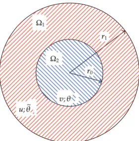
Figure 1:DomainsΩ1andΩ2and boundaries of the transmission problem.

We denote byx x1, . . . , xn a point ofΩi i 1,2whiletstands for the time variable.

The displacement in the thermoelasticity parts is denoted byu : Ω1 ×0,∞ → n,u

u1, . . . , un ui uix, t,i 1, . . . , nand v : Ω2 ×0,∞ → n,v v1, . . . , vn vi

vix, t,i 1, . . . , n, θ : Ω1×0,∞ → , and θ : Ω2×0,∞ → is the variation

of temperature between the actual state and a reference temperature, respectively.κ1,κ2are

the thermal conductivity. All the constants of the system are positive. Let us consider ann -dimensional body which is configured inΩ⊆ nn≥1.

The thermoelastic parts are given byΩ1 andΩ2, respectively. The constantsm1, m2 >

0 are the coupling parameters depending on the material properties. The boundary of Ω1

is denoted by ∂Ω1 Γ1∪Γ2 and the boundary of Ω2 by∂Ω2 Γ2. We will consider the

boundariesΓ1andΓ2of classC2in the rest of this paper. The thermoelastic parts are given by

Ω1andΩ2, respectively, that isseeFigure 1,

Ω2{x∈ n :|x|< r0}, Ω1{x∈ n :r0<|x|< r1}, 0< r0< r1. 1.5

We consider fori1,2 the operators

AiμiΔ

μiλi

∇div, 1.6

∂u ∂νAi

μi ∂u

∂ν

μiλi

divuν, 1.7

whereμi,λii1,2are the Lam´e moduli satisfyingμiλi≥0.

The initial conditions are given by

ux,0 u0x, utx,0 u1x, θx,0 θ0x, x∈Ω1, 1.8

The system is subject to the following boundary conditions:

u0, θ0 onΓ1, 1.10

uv, θθ onΓ2 1.11

and transmission conditions

μ1∇u

μ1λ1

divum1θμ2∇v

μ2λ2

divv m2θ onΓ2, 1.12

∂θ ∂νΓ2

0 onΓ2. 1.13

The transmission conditions are imposed, that express the continuity of the medium and the equilibrium of the forces acting on it. The discontinuity of the coefficients of the equations corresponds to the fact that the medium consists of two physically different materials.

Since the domain Ω ⊆ n _{is composed of two different materials, its density is}

not necessarily a continuous function, and since the stress-strain relation changes from the thermoelastic parts, the corresponding model is not continuous. Taking in consideration this, the mathematical problem that deals with this type of situation is called a transmission problem. From a mathematical point of view, the transmission problem is described by a system of partial differential equations with discontinuous coefficients. The model 1.1–

1.13 to consider is interesting because we deal with composite materials. From the economical and the strategic point of view, materials are mixed with others in order to get another more convenient material for industry see1–3 and references therein. Our purpose in this work is to investigate that the solution of the symmetrical transmission problem decays exponentially as time tends to infinity, no matter how small is the size of the thermoelastic parts. The transmission problem has been of interest to many authors, for instance, in the one-dimensional thermoelastic composite case, we can refer to the papers

4–7. In the two-, three- or n-dimensional, we refer the reader to the papers 8, 9 and references therein. The method used here is based on energy estimates applied to nonlinear problems, and the differential inequality is obtained by exploiting the symmetry of the solutions and applying techniques for the elastic wave equations, which solve the exponential stability produced by the boundary terms in the interface of the material. This methods allow us to find a Lyapunov functionalLequivalent to the second-order energy for which we have that

d

dtLt≤ −γLt. 1.14

In spite of the obvious importance of the subject in applications, there are relatively few mathematical results about general transmission problem for composite materials. For this reason we study this topic here.

2. Preliminaries

We will use the following standard notation. LetΩbe a domain in n_{. For 1 ≤p≤ ∞,L}p_Ω

are all real valued measurable functions onΩsuch that|u|pis integrable for 1 ≤p <∞and sup_x∈Ωess|ux| is finite forp∞. The norm will be written as

uLp_Ω

Ω|ux|

p_dx

1/p

, u_L∞_Ωsup ess x∈Ω

|ux|. 2.1

For a nonnegative integermand 1≤p≤ ∞, we denote byWm,p_{Ωthe Sobolev space}

of functions inLp_{Ωhaving all derivatives of order≤ mbelonging toL}p_{Ω. The norm in}

Wm,p_{Ωis given byu}

Wm,p_{Ω |α|≤m}Dαuxp_Lp_Ωdx 1/p

.Wm,2_Ω≡Hm_{Ωwith norm}

· _Hm_Ω,W0,2Ω≡L2Ωwith norm · _L2_Ω. We writeCkI, Xfor the space ofX-valued

functions which arek-times continuously differentiableresp. square integrableinI, where

I ⊆ is an interval,Xis a Banach space, andkis a nonnegative integer. We denote byOn

the set of orthogonaln×nreal matrices and bySOnthe set of matrices inOnwhich have determinant 1.

The following results are going to be used several times from now on. The proof can be found in10.

Lemma 2.1. LetG Gijn×n∈O2forn2orG Gijn×n ∈SO2forn≥3be arbitrary but

fixed. Assume thatu0,u1,θ0,v0,v1, andθ0satisfy

u0Gx Gu0x, u1Gx Gu1x, θ0Gx Gθ0x, ∀x∈Ω1,

v0Gx Gv0x, v1Gx Gv1x, θ0Gx Gθ0x, ∀x∈Ω2.

2.2

Then the solutionu,θ,v, andθof1.1–1.13has the form

uix, t xiφr, t, ∀x∈Ω1, t≥0, 2.3

θx, t ζr, t, ∀x∈Ω1, t≥0, 2.4

vix, t xiηr, t, vi0, t 0, i1,2, . . . , n, ∀x∈Ω2, t≥0, 2.5

θx, t ψr, t, ∀x∈Ω2, t≥0, 2.6

Lemma 2.2. One supposes thatu:Ω1 → n is a radially symmetric function satisfyingu|Γ1 0. Then there exists a positive constantCsuch that

∇ut_L2_Ω1≤Cdivut_L2_Ω1, t≥0. 2.7

Moreover one has the following estimate at the boundary:

|∇ut|2≤C ∂u ∂ν

2n−1

r0 |u| 2 _onΓ

2. 2.8

Remark 2.3. From2.3we have that

∇divu Δu. 2.9

The following straightforward calculations are going to be used several times from now on.

aFrom1.8we obtain

∂u ∂νA1

μ1∇u·νΩ1

μ1λ1

divuνΩ1,

∂v ∂νA2

μ2∇v·νΓ2

μ2λ2

divvνΓ2.

2.10

bUsing1.10and1.11we have that

κ1

Ω1

θΔθ d Ω1−κ1

Γ2

θ∇θ·νΓ2dΓ2−κ1

Ω1

_∇θ 2

dΩ1, 2.11

κ2

Ω2

θΔθ dΩ2κ2

Γ2

θ∇θ·νΓ2dΓ2−κ2

Ω2

|∇θ|2_dΩ

2, 2.12

m1

Ω1

∇θ·utdΩ1m1

Ω1

divutθ d Ω1−m1

Γ2

θvt·νΓ2dΓ2, 2.13

m2

Ω2

∇θ·vtdΩ2m2

Ω2

divvtθ dΩ2 m2

Γ2

cUsing1.6we have that

Ω1

μ1Δu

μ1λ1

∇divu·utdΩ1

μ1

Ω1

Δu·utdΩ1

μ1λ1

Ω1

∇divu·utdΩ1

μ1

Ω1

div∇uutdΩ1

μ1λ1

Ω1

∇divu·utdΩ1

μ1

Ω1

∇ ·ut∇udΩ1−μ1

Ω1

∇u· ∇utdΩ1

μ1λ1 Ω1

∇ ·utdivudΩ1−

μ1λ1

Ω1

divudivutdΩ1

μ1

Γ1∪Γ2

ut∇u·νΩ1dΓΩ1−

1 2μ1

d dt

Ω1

|∇u|2_dΩ 1

μ1λ1 Γ1∪Γ2

divuut·νΩ1dΓΩ1−

1 2

μ1λ1

d dt

Ω1

|divu|2dΩ1.

2.15

Thus, using1.10and1.11we have that

Ω1

A1uutdΩ1−

1 2μ1

d dt∇u

2 L2_Ω1−

1 2

μ1λ1

d

dtdivu

2 L2_Ω

1

−μ1λ1 Γ2

divuut·νΓ2dΓ2−μ1

Γ2

∇u·νΓ2utdΓ2

−1

2μ1

d dt∇u

2 L2_Ω

1−

1 2

μ1λ1

d

dtdivu

2 L2_Ω

1

−μ1λ1 Γ2

divuut·νΓ2dΓ2−μ1

Γ2

∇u·νΓ2utdΓ2.

2.16

Similarly, we obtain

Ω2

A2vvtdΩ2−1

2μ2

d dt∇v

2 L2_Ω

2−

1 2

μ2λ2

d

dtdivv

2 L2_Ω

2

μ2λ2 Γ2

divv·νΓ2dΓ2μ2

Γ2

∇v·νΓ2vtdΓ2.

2.17

3. Existence and Uniqueness

In this section we establish the existence and uniqueness of solutions to the system 1.1–

1.13. The proof is based using the standard Galerkin approximation and the elliptic regularity for transmission problem given in 11. First of all, we define what we will understand for weak solution of the problem1.1–1.13.

We introduce the following spaces:

H_Γ1

1

w∈H1Ω1:w0 onΓ1

,

V f, g∈H_Γ1

1×H

1_Ω

2:f g onΓ2

3.1

forx∈Ω⊆ n _andt≥0.

Definition 3.1. One says thatu, v,θ, θ is a weak solution of1.1–1.13if

u∈W1,∞0, T:L2Ω1

∩L∞0, T:H_Γ1

1

,

v∈W1,∞0, T:L2Ω2

∩L∞0, T:H1Ω2

,

θ∈L∞0, T:L2Ω1

∩L20, T:H_Γ1₁,

θ∈L∞0, T:L2Ω2

∩L20, T:H1Ω2

,

3.2

satisfying the identities

_T

0

Ω1

ρ1u·ϕttμ1∇u∇ϕ

μ1λ1

divudivϕm1θdivϕ

dΩ1dt

T

0

Ω2

ρ2v·χttμ2∇v∇χ

μ2λ2

divvdivχm2θdivχ

dΩ2dt

Ω1

ρ1

u1ϕ0−u0ϕt0

dΩ1

Ω2

ρ2

v1χ0−v0χt0

dΩ2,

3.3

_T

0

Ω1

−τ1θηtκ1∇θ· ∇η−m1ηdivut

dΩ1dt

_T

0

Ω2

−τ2θηtκ2∇θ· ∇η−m2ηdivvt

dΩ2dt

Ω1

θ0η0dΩ1

Ω2

θ0η0dΩ2

for allϕ, χ∈ V,η∈ C1_{0, T :H}1

Γ1,η ∈ C

1_{0, T :H}1_Ω

2, and almost everyt ∈0, T

such that

ϕT ϕtT χT χtT 0, ηT ηT 0. 3.5

The existence of solutions to the system1.1–1.13is given in the following theorem.

Theorem 3.2. One considers the following initial data satisfying

u0, u1,θ

∈H_Γ1₁Ω1×L2Ω1×L2Ω1, v0, v1, θ∈H1Ω2×L2Ω2×L2Ω2. 3.6

Then there exists only one solutionu, v,θ, θ of the system1.1–1.13satisfying

u∈W1,∞0, T:L2Ω1

∩L∞0, T:H_Γ1

1

,

v∈W1,∞0, T:L2Ω2

∩L∞0, T:H1Ω2

,

θ∈L∞0, T:L2Ω1

∩L20, T:H_Γ1

1

,

θ∈L∞0, T:L2Ω2

∩L20, T:H1Ω2

.

3.7

Moreover, if

u0, u1,θ0

∈H2Ω1∩H_Γ1₁

×H_Γ1

1×

H2Ω1∩H_Γ1₁

,

v0, v1, θ0∈H2Ω2×H1Ω2×H2Ω2

3.8

verifying the boundary conditions

u00, θ00 onΓ1,

u0v0, θ0θ0 onΓ2

3.9

and the transmission conditions

μ1∇u

μ1λ1

divum1θμ2∇v

μ2λ2

divvm2θ onΓ2,

∂θ ∂νΓ2

0 onΓ2,

then the solution satisfies

u∈L∞0, T:H2Ω1

∩W1,∞0, T:H1Ω1

∩W2,∞0, T:L2Ω1

,

v∈L∞0, T:H2Ω2

∩W1,∞0, T:H1Ω2

∩W2,∞0, T:L2Ω2

,

θ∈L∞0, T:H2Ω1

∩W1,∞0, T:L2Ω1

,

θ∈L∞0, T:H2Ω2

∩W1,∞0, T:L2Ω2

.

3.11

Proof. The existence of solutions follows using the standard Galerking approximation.

Faedo-Galerkin Scheme

Givenn∈, denote byPnandQnthe projections on the subspaces

spanϕi, χi

, spanηi, ηi

, i1,2, . . . , n 3.12

ofVandH_Γ1

1, respectively. Let us write

un, vn

n

i1

ait

ϕi, χi

,

θn, θn

n

i1

bit

ηi, ηi

, 3.13

whereun_andvn_satisfy

Ω1

ρ1untt·ϕiμ1∇un∇ϕi

μ1λ1

divundivϕim1θndivϕi

dΩ1

Ω2

ρ2vttn·χiμ2∇vn∇χi

μ2λ2

divvndivχim2θndivχi

dΩ2 0,

3.14

Ω1

τ1θntηiκ1∇θn· ∇ηi−m1ηidivunt

dΩ1

Ω2

τ2θntηiκ2∇θn· ∇ηi−m2ηidivvtn

dΩ20,

3.15

with

un0 u0, vn0 v0, unt0 u1, vnt0 v1, θn0 θ0, θn0 θ0

3.16

for almost all t ≤ T, where φ0, ψ0, η0, and η0 are the zero vectors in the respective

theory for ordinary differential equations there exists a continuous solution of this system, on some interval0, Tn. The a priori estimates that follow imply that in facttn ∞.

Energy Estimates

Multiplying3.14bya_it, summing up overi, and integrating overΩ1we obtain

d dtE

n

1t m1

Ω1

θn_divun

tdΩ1m2

Ω2

θn_divvn

tdΩ20, 3.17

where

En 1t

1 2

ρ1unt 2 L2_Ω

1μ1∇u

n2 L2_Ω1

μ1λ1

divun2_L2_Ω1

1

2

ρ2vtn 2 L2_Ω

2μ2∇v

n2 L2_Ω

2

μ2λ2

divvn2 L2_Ω

2

.

3.18

Multiplying3.15bybit, summing up overi, and integrating overΩ2we obtain

d dtE

n

2t κ1∇θn 2

L2_Ω 1

κ2∇θn2_L2_Ω2−m1

Ω1

θndivun_tdΩ1−m2

Ω2

θndivvn_tdΩ2 0,

3.19

where

En 2t

1 2τ1

θn2

L2_Ω 1

1

2 τ2θ

n2 L2_Ω

2. 3.20

Adding3.17with3.19we obtain

d dtE

n_{t κ} 1∇θn

2

L2_Ω 1

κ2 ∇θn2L2_Ω

20, 3.21

where

En_{t E}n

1un, t En2vn, t

1

2

ρ1unt 2

L2_Ω1ρ2vnt 2

L2_Ω2τ1θn 2

L2_Ω 1

τ2θn2_L2_Ω2

1

2

μ1∇un2L2_Ω1μ2∇vn2L2_Ω2

μ1λ1

divun2_L2_Ω1

μ2λ2

divvn2_L2_Ω 2

.

Integrating over0, t,t∈0, T, we have that

En_{t κ} 1

_t

0

∇θn2

L2_Ω1dtκ2

_t

0

∇θn2 L2_Ω

2dtE

n_{0. 3.23}

Thus,

un_{, u}n t,θn

is bounded in L∞0, T:H1_Ω 1

×L∞_{0, T:L}2_Ω 1

×L∞_{0, T:L}2_Ω 1

,

vn_{, v}n

t, θn

is bounded inL∞0, T:H1_Ω 2

×L∞_{0, T:L}2_Ω 2

×L∞_{0, T:L}2_Ω 2

.

3.24

Hence,

un uweakly∗ inL∞0, T:H1Ω1

,

vn vweakly∗ inL∞0, T:H1Ω2

,

un_t ut weakly∗ inL∞

0, T:L2Ω1

,

vn

t vt weakly∗ inL∞

0, T:L2_Ω 2

,

θn θweakly∗ inL∞

0, T:L2Ω1

,

θn θweakly∗ inL∞0, T:L2Ω2

.

3.25

In particular,

un_{−→ustrongly inL}2_{0, T:L}2_Ω 1

,

vn−→vstrongly inL2

0, T:L2Ω2

,

3.26

and it follows that

un−→u a.e. inΩ1,

vn−→v a.e. inΩ2.

3.27

The system1.1–1.4is a linear system, and hence the rest of the proof of the existence of weak solution is a standard matter.

The uniqueness follows using the elliptic regularity for the elliptic transmission problemsee11.We suppose that there exist two solutions u1_{, v}1_,θ1_{, θ}1_,u2_{, v}2_,θ2_{, θ}2_,

and we denote

Taking

u _t

0

U dτ, v _t

0

V dτ, θ _t

0

Θdτ, θ _t

0

Θdτ 3.29

we can see thatu, v,θ, θ satisfies1.1–1.4. Sinceu1_{, v}1_,θ1_{, θ}1_,u2_{, v}2_,θ2_{, θ}2 _{are weak}

solutions of the system we have thatu, v,θ, θ satisfies

u∈L∞0, T :H_Γ1

1

, ut∈L∞

0, T :H_Γ1

1

, utt∈L2

0, T :L2Ω1

,

v∈L∞0, T :H1Ω2

, vt∈L∞

0, T :H1Ω2

, vtt∈L2

0, T :L2Ω2

,

θ∈L20, T :H_Γ1

1

, θt∈L2

0, T :H_Γ1

1

⇒θ∈L20, T :H_Γ1

1

,

θ∈L20, T :H1Ω2

, θt∈L2

0, T :H1Ω2

⇒θ∈L20, T :H1Ω2

.

3.30

Using the elliptic regularity for the elliptic transmission problem we conclude that

u∈L∞0, T :H_Γ1₁∩H2Ω1

, v∈L∞0, T :H1Ω2∩H2Ω2

,

θ∈L∞0, T :H_Γ1

1∩H

2_Ω 1

, θ∈L∞0, T :H2Ω2

.

3.31

Thusu, v,θ, θ satisfies1.1–1.4in the strong sense. Multiplying 1.1byut,1.2byvt,

1.3byθ, and1.4byθand performing similar calculations as above we obtain Et 0, where

Et 1

2

ρ1ut2L2_Ω1μ1∇u2L2_Ω1

μ1λ1

divu2_L2_Ω1τ1θ 2

L2_Ω 1

1

2

ρ2vt2_L2_Ω

2μ2∇v

2 L2_Ω

2

μ2λ2

divv2_L2_Ω2τ2θ2_L2_Ω 2

,

3.32

which implies thatu1 _u2_,θ1 _θ2_,v1 _v2_{, andθ}1_θ2_{. The uniqueness follows.}

To obtain more regularity, we differentiate the approximate system1.1–1.4; then multiplying the resulting system bya_itandb_itand performing similar calculations as in

3.23we have that

where

En_t 1

2

ρ1un_tt2_L2_Ω1ρ2v_ttn 2

L2_Ω2τ1θn_t 2

L2_Ω 1

τ2θn_t2_L2_Ω2

1

2

μ1∇unt 2 L2_Ω

1μ2∇v

n t

2 L2_Ω

2

μ1λ1divunt 2 L2_Ω

1

μ2λ2divvnt 2 L2_Ω

2

,

Fκ1

_t

0

∇θ_tn2

L2_Ω 1

dτκ2

_t

0

∇θn τ2L2_Ω

2dτ.

3.34

Therefore, we find that

un_tt,θ_tn are bounded inL∞0, T :L2Ω1

,

v_ttn, θ_tn are bounded inL∞0, T :L2Ω2

,

un_t is bounded inL∞0, T :H1Ω1

,

v_tn is bounded inL∞0, T :H1Ω2

,

θn_t is bounded in L∞0, T :H1Ω1

,

θn_t is bounded in L∞0, T :H1Ω2

.

3.35

Finally, our conclusion will follow by using the regularity result for the elliptic transmission problemsee11.

Remark 3.3. To obtain higher regularity we introduce the following definition.

Definition 3.4. One will say that the initial datau0, v0,θ0, θ0isk-regulark≥2if

uj∈Hk−jΩ1∩H_Γ1₁, j0, . . . , k−1, uk∈L2Ω1,

θj∈Hk−jΩ1∩H_Γ1₁, j0, . . . , k−1, θk∈L2Ω2,

3.36

where the values ofujandθjare given by

ρ1uj2−A1uj−m1∇θj0 inΩ1×0,∞,

ρ2vj2−A2vj−m2∇θj 0 inΩ2×0,∞,

τ1θj1−κ1Δθj−m1divuj1 0 in Ω1×0,∞,

τ2θj1−κ2Δθj−m2divvj10 inΩ2×0,∞,

verifying the boundary conditions

uj0, θj0 onΓ1,

ujvj, θjθj onΓ2

3.38

and the transmission conditions

μ1∇u

μ1λ1

divum1θμ2∇v

μ2λ2

divvm2θ onΓ2,

∂θ ∂νΓ2

0 onΓ2

3.39

forj 0, . . . , k−1. Using the above notation we say that if the initial data isk-regular,then we have that the solution satisfies

u,θ∈

k

j0

Wj,∞0, T :Hk−jΩ1∩H_Γ1₁

,

v, θ∈

k

j0

Wj,∞0, T :Hk−jΩ2

.

3.40

Using the same arguments as inTheorem 3.2, the result follows.

4. Exponential Stability

In this section we prove the exponential stability. The great difficulty here is to deal with the boundary terms in the interface of the material. This difficulty is solved using an observability result of the elastic wave equations together with the fact that the solution is radially symmetric.

Lemma 4.1. Let one suppose that the initial datau0, v0,θ0, θ0is 3-regular; then the corresponding solution of the system1.1–1.13satisfies

dE1t

dt −κ1 ∇θ2

L2_Ω1−κ2∇θ 2 L2_Ω

2, 4.1

dE2t

dt −κ1 ∇θt

2

L2_Ω 1

−κ2∇θt2_L2_Ω

2, 4.2

whereE1t E1u, v,θ, θ, t E1₁t E2₁twith

E1 1t

1 2

ρ1ut2L2_Ω

1τ1

θ2

L2_Ω 1

μ1∇u2L2_Ω

1

μ1λ1

divu2_L2_Ω 1

,

E2 1t

1 2

ρ2vt2_L2_Ω2τ2θ_L22_Ω2μ2∇v2_L2_Ω2

μ2λ2

divv2_L2_Ω2

,

4.3

Proof. Multiplying1.1byut, integrating inΩ1, and using2.16we have that

1 2

d dt

ρ1ut2L2_Ω

1μ1∇u

2 L2_Ω

1

μ1λ1

divu2_L2_Ω 1

Γ2

μ1∇u

μ1λ1

divum1θ

ut·νΓ2dΓ2m1

Ω1

θdivutdΩ10.

4.4

Multiplying1.2byvt, integrating inΩ2, and using2.17we have that

1 2

d dt

ρ2vt2L2_Ω

2μ1∇v

2 L2_Ω

2

μ2λ2

divv2_L2_Ω 2

−

Γ2

μ2∇v

μ2λ2

divvm1θ

ut·νΓ2dΓ2m2

Ω1

θdivvtdΩ2 0.

4.5

Multiplying1.3byθ, integrating inΩ1, and using2.11we have that

τ1

2

d dt

θ2

L2_Ω2−m2

Ω1

θdivvtdΩ2κ2

Γ2

θ∇θ·νΓ2dΓ2κ2

∇θ2

L2_Ω20, 4.6

Multiplying1.4byθ, integrating inΩ2, using2.11, and performing similar calculations as

above we have that

τ2

2

d dtθ

2

L2_Ω1−m1

Ω1

θdivutdΩ1κ1

Γ2

θ∇θ·νΓ2dΓ2κ1∇θ 2

L2_Ω10. 4.7

Adding up4.4,4.5,4.6, and4.7and using1.12and1.13we obtain

dE1t

dt κ1

Ω1

_∇θ 2

dΩ1κ2

Ω2

|∇θ|2_dΩ

20, 4.8

where

E1t 1

2

ρ1ut2_L2_Ω

1ρ2vt

2 L2_Ω

2τ1

θ2

L2_Ω 1

τ2θ2_L2_Ω 2

1

2

μ1∇u2L2_Ω

1μ2∇v

2 L2_Ω

2

μ1λ1

divu2_L2_Ω

1

μ2λ2

divv2_L2_Ω 2

.

4.9

Thus

dE1t

dt −κ1 ∇θ2

L2_Ω 1

−κ2∇θ2L2_Ω2. 4.10

Lemma 4.2. Under the same hypotheses as inLemma 4.1one has that the corresponding solution of the system1.1–1.11satisfies

dE3t

dt ≤ − m1

3 divut

2 L2_Ω

1

κ2 1

2m1

Δθ2

L2_Ω 1

−δ

2μ1λ1

4ρ1 Δu 2 L2_Ω

1

δτ2 1

ρ1

2μ1λ1

τ1m1

ρ1

m2 1

2δρ1

2μ1λ1

∇θ2

L2_Ω 1

τ1

Γ2

θutt·νΓ2dΓ2−δ

Γ2

ut∂ut

∂νΓ2

dΓ2,

4.11

dE3t

dt ≤ − m2

3 divvt

2 L2_Ω

2

κ2 2

2m2Δθ 2 L2_Ω

2

− δ

2μ2λ2

4ρ2 Δv 2 L2_Ω

2

δτ₂2 ρ2

2μ2λ2

τ2m2

ρ2

m2₂

2δρ 2

2μ2λ2

∇θ2 L2_Ω

2

−τ2

Γ2

θvtt·νΓ2dΓ2−δ

Γ2

vt ∂vt

∂νΓ2

dΓ2,

4.12

whereδ,δare positive constants and

E3t −

Ω1

τ1θdivutδut·Δu

dΩ1,

E3t −

Ω2

τ2θdivvtδvt·ΔvdΩ2.

4.13

Proof. Multiplying1.1by−Δu, integrating inΩ1, and using1.10we have that

−ρ1

Ω1

utt·Δu dΩ1

2μ1λ1 Ω1

|Δu|2_dΩ 1m1

Ω1

∇θ·Δu dΩ10. 4.14

Then

−ρ1

d dt

Ω1

ut·Δu dΩ1ρ1

Ω1

ut·ΔutdΩ1

2μ1λ1 Ω1

|Δu|2_dΩ 1

m1

Ω1

∇θ·Δu dΩ10.

Hence

−ρ1 d

dt

Ω1

ut·Δu dΩ1ρ1

Ω1

∇ ·ut∇utdΩ1−ρ1

Ω1

|∇ut|2dΩ1

2μ1λ1 Ω1

|Δu|2_dΩ 1m1

Ω1

∇θ·Δu dΩ10.

4.16

Thus

−ρ1d

dt

Ω1

ut·Δu dΩ1

2μ1λ1

Δu2

L2_Ω 1

−ρ1∇ut2_L2_Ω

1−ρ1

Γ2

ut∇ut·νΓ2dΓ2m1

Ω1

∇θ·Δu dΩ10.

4.17

Hence

−d dt

Ω1

ut·Δu dΩ1−

2μ1λ1

ρ1 Δu 2 L2_Ω

1∇ut

2 L2_Ω

1

Γ2

ut

∂ut

νΓ2

dΓ2−

m1

ρ1

Ω1

∇θ·Δu dΩ1.

4.18

Therefore

−d dt

Ω1

ut·Δu dΩ1≤ −

2μ1λ1

2ρ1 Δu 2 L2_Ω

1

m2 1

2ρ1

2μ1λ1

∇θ2

L2_Ω 1

∇ut2_L2_Ω

1

Γ2

ut∂ut

∂νΓ2

dΓ2.

4.19

Similarly, multiplying1.2by−Δv, integrating inΩ2, and performing similar calculations as

above we obtain

−d dt

Ω2

vt·Δv dΩ2≤ −

2μ2λ2

2ρ2 Δv 2 L2_Ω2

m2₂

2ρ2

2μ2λ2

∇θ2 L2_Ω2

∇vt2_L2_Ω

2−

Γ2

vt∂vt

∂νΓ2

dΓ2.

4.20

Multiplying1.3by−divutand integrating inΩ1we have that

−τ1

Ω1

θtdivutdΩ1κ1

Ω1

ΔθdivutdΩ1m1

Ω1

Hence

−τ1d

dt

Ω1

θtdivutdΩ1τ1

Ω1

θdivuttdΩ1m1divut2_L2_Ω1κ1

Ω1

ΔθdivutdΩ10.

4.22

Then

−τ1d

dt

Ω1

θdivutdΩ1τ1

Ω1

∇ ·θu tt

dΩ1−τ1

Ω1

∇θ·uttdΩ1

m1divut2_L2_Ω1κ1

Ω1

ΔθdivutdΩ1 0.

4.23

Using1.10and2.9and performing similar calculations as above we obtain

−τ1 d

dt

Ω1

θdivutdΩ1−m1divut2_L2_Ω1τ1

Ω1

∇θ·uttdΩ1

τ1

Γ2

θutt·νΓ2dΓ2−κ1

Ω1

ΔθdivutdΩ1.

4.24

Replacing1.1in the above equation we obtain

−τ1

d dt

Ω1

θdivutdΩ1−m1divut2L2_Ω

1

τ1

ρ1

2μ1λ1 Ω1

∇θΔu dΩ1

τ1m1

ρ1

Ω1

_∇θ 2

dΩ1−κ1

Ω1

ΔθdivutdΩ1τ1

Γ2

θutt·νΓ2dΓ2.

4.25

On the other hand

κ1

Ω1

ΔθdivutdΩ1 ≤

κ2 1

2m1

Δθ2

L2_Ω1

m1

2 divut

2 L2_Ω

1. 4.26

Therefore

−τ1

d dt

Ω1

θdivutdΩ1≤ −

m1

2 divut

2 L2_Ω1

τ1

ρ1

m1∇θ 2

L2_Ω1

κ2₁

2m1

Δθ2

L2_Ω1

τ1

ρ1

2μ1λ1 Ω1

∇θΔu dΩ1τ1

Γ2

θutt·νΓ2dΓ2.

Multiplying1.4by−divvt, integrating inΩ2, and performing similar calculations as above

we obtain

−τ2d

dt

Ω2

θdivvtdΩ2≤ − m2

2 divvt

2 L2_Ω

2

τ2

ρ2

m2∇θ2_L2_Ω

2

κ2 2

2m2 Δθ 2 L2_Ω

2

τ2

ρ2

2μ2λ2 Ω2

∇θΔv dΩ2−τ2

Γ2

θvtt·νΓ2dΓ2.

4.28

Adding4.19with4.27we have that

dE3t

dt ≤ − m1

2 divut

2 L2_Ω

1τ1

Γ2

θutt·νΓ2dΓ2

Γ2

ut∂ut

∂νΓ2

dΓ2

−

2μ1λ1

2 ρ1 Δu 2 L2_Ω

1∇ut

2 L2_Ω

1

κ2₁

2m1

Δθ2

L2_Ω 1

τ1

ρ1

2μ1λ1 Ω1

∇θΔu dΩ1

τ1m1

ρ1

m2₁

2ρ1

2μ1λ1

∇θ2

L2_Ω 1

.

4.29

Adding4.20with4.28we have that

dE3t

dt ≤ − m2

2 divvt

2

L2_Ω2−τ2

Γ2

θvtt·νΓ2dΓ2−

Γ2

vt∂vt

∂νΓ2

dΓ2

−

2μ2λ2

2ρ2 Δv 2 L2_Ω

2∇vt

2 L2_Ω

2

κ2 2

2 m2 Δθ 2 L2_Ω

2

τ2

ρ2

2μ2λ2 Ω2

∇θΔv dΩ2

τ2m2

ρ2

m22

2ρ2

2μ2λ2

∇θ2 L2_Ω

2.

4.30

Moreover, byLemma 2.2, there exist positive constantsC1,C2such that

∇utL2_Ω

1≤C1divut

2 L2_Ω

1, ∇vtL2Ω2≤C2divvtL2Ω2. 4.31

Therefore we obtain

dE3t

dt ≤ − m1

3 divut

2 L2_Ω

1τ1

Γ2

θutt·νΓ2dΓ2

κ2 1

2m1

Δθ2

L2_Ω 1

−δ

2μ1λ1

4ρ1 Δu 2 L2_Ω

1 δτ2 1 ρ1

2μ1λ1

τ1m1

ρ1

m2 1

2δρ1

2μ1λ1

∇θ2

L2_Ω1.

Similarly

dE3t

dt ≤ − m2

3 divvt

2 L2_Ω

2−τ2

Γ2

θvtt·νΓ2dΓ2

κ2 2

2m2 Δθ 2 L2_Ω

2

− δ

2μ2λ2

4ρ2 Δv 2 L2_Ω

2

δτ2 2

ρ2

2μ2λ2

τ2m2

ρ2

m2 2

2δρ2

2μ2λ2

∇θ2 L2_Ω

2.

4.33

The result follows.

Lemma 4.3. Under the same hypotheses ofLemma 4.1one has that the corresponding solution of the system1.1–1.13satisfies

dE4t

dt ≤ − κ1

2

2μ1λ1Δθ 2

L2_Ω 1

−κ2

2

ρ1

ρ2

2μ2λ2

Δθ2

L2_Ω 2

−ρ1

2μ1λ1 Γ2

utt ∂ut

∂νΓ2

dΓ2ρ1

2μ2λ2 Γ2

vtt∂vt

∂νΓ2

dΓ2

C

ε3

∇θ2

L2_Ω1

C ε3∇θ

2

L2_Ω22εdivvt2L2_Γ2,

4.34

with

E4t

2μ1λ1

E1

4t

ρ1

ρ2

2μ2λ2

E2

4t,

E1 4t

1 2

ρ1∇ut2L2_Ω1

2μ1λ1

Δu2

L2_Ω1τ1∇θ 2

L2_Ω 1

,

E2 4t

1 2

ρ2∇vt2_L2_Ω

2

2μ2λ2

Δv2

L2_Ω

2τ2∇θ

2 L2_Ω

2

,

4.35

whereε,CCm1, μ1, λ1andCCm2, μ2, λ2are positive constants.

Proof. Multiplying1.1 by−2μ1 λ1Δut, integrating inΩ1, using 2.9, and performing

straightforward calculations we have that

1 2ρ1

2μ1λ1

d dt∇ut

2 L2_Ω

1ρ1

2μ1λ1 Γ2

utt∇ut·νΓ2dΓ2

1

2

2μ1λ1

2d

dtΔu

2 L2_Ω

1m1

2μ1λ1 Ω1

∇θ·ΔutdΩ10.

Using1.10we obtain

1 2

2μ1λ1

d dt

ρ1∇ut2L2_Ω1

2μ1λ1

Δu2

L2_Ω1

−ρ1

2μ1λ1 Γ2

utt

∂ut

∂νΓ2

dΓ2−m1

2μ1λ1 Ω1

∇θ·ΔutdΩ1.

4.37

Multiplying 1.2 by −ρ1/ρ22μ2 λ2Δvt, integrating in Ω2, and performing similar

calculations as above we obtain

1 2

ρ1

ρ2

2μ2λ2

d dt

ρ2∇vt2_L2_Ω

2

2μ2λ2

Δv2

L2_Ω 2

ρ1

2μ2λ2 Γ2

vtt∂vt

∂νΓ2

dΓ2−m2

ρ1

ρ2

2μ2λ2 Ω2

∇θ·ΔvtdΩ2.

4.38

Multiplying1.3by−2μ1λ1Δθand integrating inΩ1, we have that

−τ1

2μ1λ1 Ω1

θtΔθ d Ω1κ1

2μ1λ1Δθ 2

L2_Ω 1

m1

2μ1λ1 Ω1

divutΔθ d Ω10.

4.39

Performing similar calculations as above we obtain

1 2τ1

2μ1λ1

d dt

∇θ2

L2_Ω 1

−κ1

2μ1λ1Δθ 2

L2_Ω 1

−m1

2μ1λ1 Ω1

divutΔθ d Ω1

−τ1

2μ1λ1 Γ2

θ ∂θ

∂νΓ2

dΓ2.

4.40

Multiplying 1.4 by −ρ1/ρ22μ2 λ2Δθ, integrating in Ω1, and performing similar

calculation as above we obtain

1 2τ2

ρ1

ρ2

2μ2λ2

d dt∇θ

2

L2_Ω2−κ2

ρ1

ρ2

2μ2λ2

Δθ2

L2_Ω2

−m2

ρ1

ρ2

2μ2λ2 Ω2

divvtΔθ dΩ2

τ2

2μ2λ2 Γ2

θ ∂θ ∂ν_Γ2dΓ2.

Adding 4.37, 4.38, 4.40, and 4.41, using 1.13, and performing straightforward calculations we obtain

dE4t

dt −κ1

2μ1λ1 Δθ 2

L2_Ω 1

−κ2

ρ1

ρ2

2μ2λ2

∇θ2

L2_Ω 2

−ρ1

2μ1λ1 Γ2

utt

∂ut

∂νΓ2

dΓ2ρ1

2μ2λ2 Γ2

vtt

∂vt

∂νΓ2

dΓ2

m1

2μ1λ1 Γ2

∂θ ∂νΓ2

divutdΓ2−m2

2μ2λ2 Γ2

∂θ ∂νΓ2

divvtdΓ2,

4.42

with

E4t

2μ1λ1

E1

4t

ρ1

ρ2

2μ2λ2

E2

4t,

E1 4t

1 2

ρ1∇ut2_L2_Ω

1

2μ1λ1

Δu2

L2_Ω

1τ1

∇θ2

L2_Ω 1

,

E2 4t

1 2

ρ2∇vt2L2_Ω2

2μ2λ2

Δv2

L2_Ω2τ2∇θ2L2_Ω 2

.

4.43

Using the Cauchy inequality we have that

Γ2

∂θ ∂νΓ2

divutdΓ2 ≤ 1

4ε

Γ2

∂θ

∂νΓ2

2dΓ2ε

Γ2

|divut|2dΓ2, 4.44

and, from trace and interpolation inequalities, we obtain

Γ2

∂θ ∂νΓ2

divutdΓ2≤ C1

4ε

Ω1

_∇θ 2

dΩ1

1/2

Ω1

_Δθ 2

dΩ1

1/2

ε

Γ2

|divut|2dΓ2

≤ C ε3

Ω1

_∇θ 2

dΩ1ε

Ω1

_Δθ 2

dΩ1ε

Γ2

|divut|2dΓ2.

4.45

Similarly

Γ2

∂θ

∂ν_Γ2divvtdΓ2≤ C ε3

Ω1

|∇θ|2_dΩ 1ε

Ω1

|Δθ|2_dΩ 1ε

Γ2

Replacing in the above equation we obtain

dE4t

dt ≤ −κ1

2μ1λ1Δθ 2

L2_Ω1−κ2

ρ1

ρ2

2μ2λ2

Δθ2

L2_Ω2

−ρ1

2μ1λ1 Γ2

utt

∂ut

∂νΓ2

dΓ2ρ1

2μ2λ2 Γ2

vtt

∂vt

∂νΓ2

dΓ2

C

ε3

Ω1

_∇θ 2

dΩ1ε

Ω1

_Δθ 2

dΩ1ε

Γ2

|divut|2dΓ2

C

ε3

Ω1

|∇θ|2_dΩ 1ε

Ω1

|Δθ|2_dΩ 1ε

Γ2

|divvt|2dΓ2.

4.47

The result follows.

We introduce the following integrals:

I1

Ω1

ρ1utt

q· ∇utdΩ1,

I2

Ω1

ρ1utth· ∇utdΩ1,

4.48

where

q∈C2Ω1∪Ω2

3

, qx ⎧ ⎨ ⎩

ν if x∈Γ1,

0 if x∈Ω1∪Ω2,

h∈C2Ω1∪Ω2

3

, hx ⎧ ⎨ ⎩

0 if x∈Ω1\Ω3,

x if x∈Ω2,

4.49

withΩ3 Ω2∪∪x∈Γ2εx, whereεxis a ball with centerxand radiusε.

Lemma 4.4. Under the same hypotheses as inLemma 4.1one has that the corresponding solution of the system1.1–1.13satisfies

dI1t

dt ≤ −k0 ∂ut

∂ν_Γ2 2

L2_Γ 2

Ck0

∇ut2L2_Ω

1Δu

2 L2_Ω

1

∇θt

2

L2_Ω 1

, 4.50

dI2t

dt ≤ − r0

2

2μ1λ1

∂ut

∂νΓ2

2

L2_Γ2

ρ1utt2_L2_Γ2

n−1

2

2μ1λ1

ut2L2_Γ2C

∇ut2L2_Ω1Δu_L22_Ω1∇θt 2

L2_Ω 1

,

4.51

Proof. Using Lemma A.1, takinghas above,ϕut,fm1∇θt, andΩ Ω1, we obtain

dI2t

dt ≤

2μ1λ1 Γ

∂ut

∂νΓ

n

i1

hi∂ut

∂xi

dΓ 1

2ρ1

Γ|utt| 2

n

i1

hiνiΓ

dΓ

−1

2

2μ1λ1

Γ|∇ut| 2

_n

i1

hiνiΓ

dΓ

−1

2

Ω1

ρ1|utt|2−

2μ1λ1

|∇ut|2

n

11

∂hi

∂xi

dΩ1

−2μ1λ1 Ω1

∇ut

_n

i1

∇hi

∂ut

∂xi

dΩ1m1

Ω1

∇θt

_n

i1

hi

∂ut

∂xi

dΩ1.

4.52

Applying the hypothesis onhand since

h−r0νΓ2, r0|x|, ∀x∈Γ2, r0diamΩ2,

h0, ∀x∈Γ1,

4.53

we have that

dI2t

dt ≤ −r0

2μ1λ1 Γ2

∂ut

∂νΓ2

2dΓ2−

r0

2ρ1

Γ2

|utt|2dΓ2

r0

2

2μ1λ1 Γ2

|∇ut|2dΓ2

−1

2

Ω1

ρ1|utt|2−

2μ1λ1

|∇ut|2

dΩ1

−2μ1λ1 Ω1

|∇ut|2dΩ1m1

Ω1

∇θth· ∇utdΩ1.

4.54

Using2.8and the Cauchy-Schwartz inequality in the last term and performing straightfor-ward calculations we obtain

dI2t

dt ≤ − r0

2

Γ2

2μ1λ1 ∂ut

∂νΓ2

2ρ1|utt|2

dΓ2

n−1

2

2μ1λ1 Γ2

|ut|2dΓ2C

Ω1

|utt|2|∇ut|2 ∇θt 2

dΩ1.

4.55

Finally, considering1.1and applying the trace theorem we obtain

utL2_Γ

2≤C∇u tL2Ω1, 4.56

We now introduce the integrals

I3t ρ2

Ω2

vttx· ∇vtdΩ2, Φt I3t

n−1 2 ρ2

Ω2

vt·vttdΩ2. 4.57

Lemma 4.5. With the same hypotheses as inLemma 4.1, the following equality holds:

dΦt

dt

r0

2

2μ2λ2∂vt

∂νΓ2

2

L2_Γ2

ρ2vtt2_L2_Γ2

n−1

2μ2λ2

2

Γ2

vt

∂vt

∂νΓ2

dΓ2

n−12μ2λ2

2 vt

2 L2_Γ2

−1

2

ρ2vtt2L2_Ω

2

2μ2λ2

∇vt2L2_Ω 2

n−1

2 m2

Ω2

vt· ∇θtdΩ2.

4.58

Proof. Differentiating1.2in thet-variable we have that

ρ2vttt

2μ2λ2

Δvtm2∇θt. 4.59

Multiplying the above equation byvtand integrating inΩ2we obtain

ρ2

Ω2

vt·vtttdΩ2

2μ2λ2 Ω2

vt·ΔvtdΩ2m2

Ω2

vt· ∇θtdΩ2. 4.60

Hence

ρ2

d dt

Ω2

vt·vttdΩ2ρ2

Ω2

|vtt|2dΩ2ρ2

Ω2

vt·vtttdΩ2

ρ2

Ω2

|vtt|2dΩ2

2μ2λ2 Ω2

vt·ΔvtdΩ2

m2

Ω2

vt· ∇θtdΩ2

ρ2vtt2_L2_Ω

2−

2μ2λ2

∇vt2_L2_Ω 2

2μ2λ2 Γ2

vt

∂vt

∂ν_Γ2dΓ2m2

Ω2

vt· ∇θtdΩ2.

On the other hand, using Lemma A.1 forhx,ϕvt,f0, andΩ Ω2we obtain

dI3t

dt

r0

2

2μ2λ2

∂vt

∂νΓ2

2

L2_Γ 2

ρ2vtt2L2_Γ 2

−n−1

2μ2λ2

2 vt

2 L2_Γ2

n−1 2

2μ2λ2

∇vt2_L2_Ω2−ρ2vtt2_L2_Ω2

−1

2

2μ2λ2

∇vt2_L2_Ω

2ρ2vtt

2 L2_Ω

2

.

4.62

Multiplying4.61byn−1/2 and adding with4.62we obtain

d dtΦt

r0

2

2μ2λ2

∂vt

∂νΓ2

2

L2_Γ 2

ρ2vtt2L2_Γ 2

n−1

2μ2λ2

2

Γ2

vt∂vt

∂νΓ2

dΓ2

n−12μ2λ2

2 vt

2 L2_Γ

2

−1

2

ρ2vtt2_L2_Ω2

2μ2λ2

∇vt2_L2_Ω2

n−1

2 m2

Ω2

vt· ∇θtdΩ2.

4.63

The result follows.

We introduce the integral

Mt E4t

m1

2μ1λ1

2κ1 E3

t m2

2μ2λ2

2κ2

E3t δ1I1t δ2I2t, 4.64

whereδ1andδ2are positive constants.

Lemma 4.6. Under the same hypotheses as inLemma 4.1one has that the corresponding solution of the system1.1–1.13satisfies

dMt dt ≤ −

κ1

4

2μ1λ1Δθ 2

L2_Ω1−

κ2

4

ρ1

ρ2

2μ2λ2

Δθ2

L2_Ω2

−

C1−δ1Cκ0−δ2c−

δCpc

2

∇ut2_L2_Ω

1−C2∇vt

2 L2_Ω

2

−δm1

2μ1λ1

2

32ρ1κ1 Δu 2 L2_Ω1−

δm2

2μ2λ2

2

32ρ2κ2

ρ1

ρ2Δv 2 L2_Ω2

Cε

∇θ2

L2_Ω 1

∇θt 2

L2_Ω 1

Cε

∇θ2

L2_Ω

2∇θt

2 L2_Ω

2