Please cite this article as: H. Rasay, M. S. Fallahnezhad, Y. Zaremehrjerdi, Application of Multivariate Control Charts for Condition Based Maintenance, International Journal of Engineering (IJE), IJE TRANSACTIONS A: Basics Vol. 31, No. 4, (April 2018) 597-604
International Journal of Engineering
J o u r n a l H o m e p a g e : w w w . i j e . i rApplication of Multivariate Control Charts for Condition Based Maintenance
H. Rasay, M. S. Fallahnezhad*, Y. Zaremehrjerdi
Department of Industrial Engineering, Yazd University, Yazd, Iran
P A P E R I N F O
Paper history:
Received 28 May 2017
Received in revised form 26 September 2017 Accepted 12 October 2017
Keywords: Condition Monitoring Condition Based Maintenance Statistical Process Control Multivariate Control Chart
A B S T R A C T
Condition monitoring is the foundation of a condition based maintenance (CBM). To relate the information obtained from the condition monitoring to the actual state of the system, it is usually required a stochastic model. On the other hand, considering the interactions and similarities that exist between CBM and statistical process control (SPC), the integrated models for CBM and SPC have been developed. These models apply control charts as a condition monitoring technique, and the inference about the operational states of the system is based on the collected information about the quality of the produced items. Finally, it is decided whether to implement certain type of maintenance actions. This paper describes the application of multivariate control charts as a condition monitoring technique for CBM purposes. To this end, an integrated model is developed, while it is used a chi-square control chart. Also, to determine the inspection time points, a constant hazard policy is applied.
doi: 10.5829/ije.2018.31.04a.11
NOMENCLATURE
Ri
Expected revenue for the system operation per time unit, when the system is in operational state i (i=0,1) (R0>R1)
t Equipment age at the start of each production cycle
CQC Sampling inspection cost 𝑘 dimension of the observations
CPM Preventive maintenance cost ti (
i=1,..,m-1)
time points of the sampling inspection (they are the decision variables of the model)
CCM Corrective maintenance cost Probability of type I error for the control chart
CI The cost of the maintenance inspection Probability of type II error for the control chart
ZPM Expected time required for the preventive maintenance N
The sample size in each sampling inspection (it is a decision variable of the model)
ZCM Expected time required for the Corrective maintenance tm Maximum duration of each production cycle (decision variable)
ZI Expected time required for the maintenance inspection m
Maximum number of the inspection periods (decision variable)
f(t) Density function of time of quality shift E[T0] The expected time that the system operates in state 0
during each production cycle
F(t) Cumulative distribution function (c.d.f) of the time of
quality shift (𝐹̅(𝑡) = 1 − 𝐹(𝑡)) 𝑃𝑃𝑀 Probability that a production cycle is terminated due to the preventive maintenance
𝜑𝑖(𝑡) Density function of time to failure state if the system is in state i (i=0,1) at t=0 𝑃𝐶𝑀 Probability that a production cycle is terminated due to the corrective maintenance
𝜙𝑖(𝑡)
Cumulative distribution function (c.d.f) of time to failure state if the system is in state i (i=0,1) at t=0
1. INTRODUCTION1
In the most models developed for condition based maintenance (CBM), it is usually assumed that the system has several operational states plus a failure state. In the failure state the system stops, thus, this state is
*Corresponding Author’s Email: [email protected] (M. S. Fallahnezhad)
operational state of the system is not observable and the obtained information in the condition monitoring only partially informs about the system state. This type of condition monitoring is called indirect condition monitoring. Hence, in the indirect condition monitoring, it is necessary to establish a stochastic model for relating the obtained information from the condition monitoring to the actual system state [1-5].
On the other hand, as stated by many authors, there are great interactions and interrelations between CBM and SPC [1, 6-8]. Considering the interactions and similarities that exist between CBM and SPC, the integrated models for CBM and quality control have been developed. These models usually apply the control chart as a condition monitoring technique. In these models, the inference about the operational states of the system is based on the collected information about the quality of the produced items. Finally, it is decided whether or not to implement certain types of maintenance actions. Indeed, the integrated models for CBM and SPC have been developed based on the fact that the product quality can partially indicates the actual operational state of the system.
Wang [2] used the multivariate Bayesian control chart for CBM. Panagiotidou and Tagaras [6], Panagiotidou and Tagaras [9] proposed an integrated model for CBM and SPC based on the 𝑋̅ control chart. Yin et al. [10] developed an integrated model for CBM and SPC, while it was used a delayed monitoring for the CBM purposes. Panagiotidou and Nenes [11] used an adaptive Shewhart chart for the CBM purposes and proposed an integrated model for maintenance planning and economical design of an adaptive Shewhart chart. Ardakani et al. [12] developed an integrated maintenance planning and SPC model based on the multivariate exponentially weighted moving average (MEWMA) chart. Jamshidi and Madie [13] proposed an integrated model for maintenance and work-rest scheduling. Lie et al. [14], according to the geometric process, proposed a model for CBM and SPC. Wu and Makis [1] proposed a model for the economic design of a chi-square control chart for a CBM application. Wu and Makis assumed that the system has three states including: in-control state, out-of-control state and failure states. Also, transition time between these states is based on the exponential distribution, and it is used Markov chain for deriving the integrated model.
In this paper, the proposed model by Wu and Makis is developed based on three main contributions:
1. while in the Wu and Makes’ study, the deterioration mechanism is assumed to follow the exponential distribution; we place no restrictive assumption on the deterioration mechanism of the system. In other words, the time to quality shift as well as the time to the failure state from each operational states were assumed as a general continuous distribution function.
2. considering the memory less property of the exponential distribution, Wu and Makis applied Markov chain in deriving their model. While in this paper, developing the integrated CBM and SPC model is based on the recursive equations and renewal reward process.
3. the proposed model in this paper is applicable for different types of inspection policy, while the proposed model by Wu and Makis is based on the fixed time interval inspection policy. Thus, by releasing many assumptions of the Wu and Makis’ model, our proposed model can be applied in more practical situations and has a wider application domain. Indeed, the proposed model by Wu and Makis can be considered as a special state of the proposed model in this paper.
The rest of the paper is organized as follows: section 2 describes the considered system. In section 3, the proposed model is derived. In section 4, the proposed model in section 3 is applied for a situation that a chi-square control chart is used as a condition monitoring technique. Also, constant hazard policy is introduced in this section. Section 5 presents two examples of the application of the model. Some sensitivity analyses are presented in section 6. Finally, section 7 concludes the paper.
2. DESCRIPTION
Consider a production process or a single production machine which may operate under different conditions. Specifically, the system has two operational states, as well as a failure state that is non-operational. The operational states include in-control state (denoted as state 0) and out-of-control state (denoted as state 1). Every production cycle starts from the in-control state and zero equipment age. The system may shift from state 0 to state 1 or directly shift from state 0 to the failure state due to the usage and age. Having shifted the system to state 1, if this state is not identified, the system eventually shifts from state 1 to the failure state.
The system operation in state 1 is undesirable in comparison with its operation in state 0, due to the lower level of the produced item quality, the lower revenue and the higher chance for the system complete failure. In the failure state, the system stops and cannot produce the item. No matter what is the operational states, the system may transit from an operational state to the failure state. It is assumed that the transition time from state 0 to 1, from state 0 to the failure state and from state 1 to the failure state are based on the probability functions that follow a general continuous distributions. Also, the failure rate of the system in state 1 is higher than the failure rate in state 0.
system is in state 1 or 0) is based on the condition monitoring. More specifically, the operational condition of the system is inferred based on the quality of the produced item. Condition monitoring is implemented as follows: at the specific time points, such as t1, t2,…, tm-1, that are decision variables in the model, a sample with size n is taken from the produced item of the system.
Based on the information collected from the quality of this sample, an appropriate statistic is computed and plotted on a suitable multivariate control chart. If the value of this statistic exceeds the control limits of the chart, the chart alarms meaning that the system probably operates in the out-of-control state. To determine the actual state of the system, an error free inspection is conducted after releasing each alarm from the control chart. This inspection is called maintenance inspection to distinguish it from the sampling inspection. If the maintenance inspection indicates that the system is in state 1 then preventive maintenance (PM) is implemented on the system. But if the maintenance inspection concludes that the system state is 0 (in other words the chart alarm is incorrect) then the system will continue its operation without any further actions.
Once the system transits to the failure state, the corrective maintenance (CM) is conducted and the system renews. It is possible for the system to operate without transiting to the failure state until the end of the production cycle (at time point tm). In this situation the system may be in state 0 or 1 however, regardless of the system state at tm , the PM is implemented. Thus, PM is conducted in two general situations: 1- after releasing a true out-of-control signal from the control chart and 2- if the system reaches the time point tm. Hence, two types of maintenance is implemented on the system: PM and CM. It is assumed that both types of the maintenance are perfect such that they can renew the system to the as-good-as new state. Once each type of the maintenance is implemented on the system, the system renews and a new production cycles starts.
3.MODEL DEVELOPMENT
In this section, based on the renewal reward process and recursive equations, an integrated stochastic model is developed for CBM and SPC
3. 1. System Evolution During an Inspection Interval In each inspection interval, six different scenarios are possible for the system operation. These scenarios are illustrated in Table 1. Also, in this table, the pertinent
3. 2. System State at the Start of Each Inspection Interval Let denote 𝑃𝑡0𝑖 , 𝑃𝑡1𝑖 as the probabilities that,
immediately after inspection at ti, the system operates in
the in-control state or out-of-control state, respectively. In this subsection, the computation of these probabilities is described. 𝑃𝑡0𝑖 is given by:
𝑃𝑡𝑖
0= 𝐹̅(𝑡
𝑖)Φ̅0(𝑡𝑖); ; 1 ≤ 𝑖 ≤ 𝑚 (1)
This equation is obtained based on the fact that the system operates in state 0 at 𝑡𝑖, if and only if the time to
quality shift as well as the transition time from state 0 to the failure state be greater that 𝑡𝑖. 𝑃𝑡1𝑖 is calculated based
on this recursive formula: 𝑃𝑡𝑖
1= 𝛽𝑃 𝑡𝑖−1
0 . 𝑃(𝑏
𝑡𝑖−1) + 𝛽𝑃𝑡𝑖−1 1 . 𝑃(𝑒
𝑡𝑖−1); 1 ≤ 𝑖 ≤ 𝑚 − 1 (2)
This equation is obtained as follows: with respect to Table 1, it is clear that the system will operate in state 1 at 𝑡𝑖 in two cases: (1) if the system is in state 0 at 𝑡𝑖−1 ,
scenario b occurs and the control chart cannot identify this state; or (2) the system is in state 1 at 𝑡𝑖−1, scenario
e occurs and the control chart cannot identify this state. It is assumed that there is no sampling inspection at tm. Hence, for the last inspection time we have:
𝑃𝑡𝑚
1 = 𝑃 𝑡𝑚−1
0 . 𝑃(𝑏
𝑡𝑚−1) + 𝑃𝑡𝑚−1
1 . 𝑃(𝑒
𝑡𝑚−1) (3)
Both maintenance types are assumed to be perfect. Hence, at the start of each production cycle the following equation is held:
𝑃𝑡0
0 = 1; 𝑃 𝑡0
1 = 0 (4)
Equation (4) indicates that, as it was assumed, each production cycle starts with a new zero-age system. In other words, at the start of each production cycle the system is in state 0.
3. 3. Expected In-control and out-of-control Time Expected time during each production cycle that the system operates in the in-control state can be obtained using the following equation:
𝐸[𝑇0] = ∫ 𝐹̅(𝑡)𝜙̅0(𝑡)𝑑𝑡 𝑡𝑚
0 (5)
Expected time during the inspection interval (𝑡𝑖−1, 𝑡𝑖)
that the system operates in the out-of-control state is denoted by 𝑇1𝑖 . Using the following equation, 𝑇1𝑖 can be
computed:
𝑇1𝑖= 𝑃(𝑡𝑖−10 ) [∫ (𝑡𝑖− 𝑡) 𝑓(𝑡) 𝐹̅(𝑡𝑖−1)
𝜙̅0(𝑡) 𝜙̅0(𝑡𝑖−1) 𝑡𝑖
𝑡𝑖−1
𝜙̅1(𝑡𝑖) 𝜙 ̅1(𝑡)𝑑𝑡] +
𝑃(𝑡𝑖−10 ) ∫ (𝑡′− 𝑡) 𝑓(𝑡) 𝐹̅(𝑡𝑖−1) 𝑡𝑖
𝑡𝑖−1
𝜙̅0(𝑡) 𝜙̅0(𝑡𝑖−1)∫
𝜑1(𝑡′) 𝜙̅1(𝑡) 𝑡𝑖
𝑡 𝑑𝑡
′𝑑𝑡
+ 𝑃(𝑡𝑖−11 )[
𝜙̅1(𝑡𝑖) 𝜙
̅1(𝑡𝑖−1)(𝑡𝑖− 𝑡𝑖−1) + ∫ (𝑡 − 𝑡𝑖−1) 𝜑1(𝑡) Φ̅1(𝑡𝑖−1) 𝑡𝑖
𝑡𝑖−1 𝑑𝑡];
1 ≤ 𝑖 ≤ 𝑚
(6)
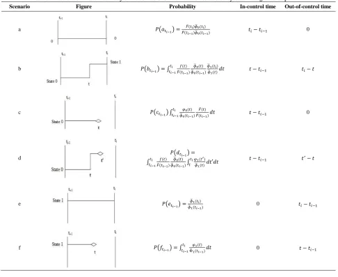
TABLE 1. Different scenarios that may occur for the evolution of the considered system during each inspection interval
Scenario Figure Probability In-control time Out-of-control time
a 𝑃(𝑎𝑡𝑖−1) =
𝐹̅(𝑡𝑖)𝜙̅0(𝑡𝑖)
𝐹̅(𝑡𝑖−1)𝜙̅0(𝑡𝑖−1) 𝑡𝑖− 𝑡𝑖−1 0
b 𝑃(𝑏𝑡𝑖−1) = ∫
𝑓(𝑡) 𝐹̅(𝑡𝑖−1)
𝜙 ̅0(𝑡) 𝜙 ̅0(𝑡𝑖−1) 𝑡𝑖
𝑡𝑖−1
𝜙̅1(𝑡𝑖)
𝜙̅1(𝑡)𝑑𝑡 𝑡 − 𝑡𝑖−1 𝑡𝑖− 𝑡
c 𝑃(𝑐𝑡𝑖−1) ∫
𝜑0(𝑡) 𝜙 ̅0(𝑡𝑖−1)
𝐹̅(𝑡) 𝐹̅(𝑡𝑖−1) 𝑡𝑖
𝑡𝑖−1 𝑑𝑡 𝑡 − 𝑡𝑖−1 0
d 𝑃(𝑑𝑡𝑖−1) =
∫ 𝑓(𝑡) 𝐹̅(𝑡𝑖−1) 𝑡𝑖 𝑡𝑖−1
𝜙̅0(𝑡) 𝜙̅0(𝑡𝑖−1)∫
𝜑1(𝑡′) 𝜙̅1(𝑡) 𝑡𝑖
𝑡 𝑑𝑡′𝑑𝑡
𝑡 − 𝑡𝑖−1 𝑡′− 𝑡
e 𝑃(𝑒𝑡𝑖−1) =
𝜙̅1(𝑡𝑖)
𝜙̅1(𝑡𝑖−1) 0 𝑡𝑖− 𝑡𝑖−1
f 𝑃(𝑓𝑡𝑖−1) = ∫
𝜑1(𝑡) Φ̅1(𝑡𝑖−1) 𝑡𝑖
𝑡𝑖−1 𝑑𝑡 0 𝑡 − 𝑡𝑖−1
3. 4. Performance Probability of Each Type of the Maintenance Probability of performance of the PM action at the end of the inspection interval (𝑡𝑖−1, 𝑡𝑖) is
denoted by 𝑃𝑃𝑀𝑖 . Using the following equation 𝑃𝑃𝑀𝑖 can
be calculated: 𝑃𝑃𝑀𝑖 = 𝑃𝑡𝑖−1
0 (1 − 𝛽)𝑃(𝑏
𝑡𝑖−1) + 𝑃𝑡𝑖−1
1 (1 −
𝛽)𝑃(𝑒𝑡𝑖−1); 1 ≤ 𝑖 ≤ 𝑚 − 1
(7)
This equation is obtained as follows: with respect to Table 1, it is clear that at ti, PM is implemented on the system in two cases: (1) if the system is in state 0 at 𝑡𝑖−1
, scenario b occurs and the control chart identify this state; or (2) the system is in state 1 at 𝑡𝑖−1, scenario e
occurs and the control chart identify this state. At time point tm , neither maintenance inspection nor sampling inspection is implemented on the system. Thus, the probability for conducting the PM action at tm is computed as follows:
𝑃𝑃𝑀𝑚 = 𝑃𝑡𝑚−1
0 [𝑃(𝑎
𝑚−1) + 𝑃(𝑏𝑚−1)] +
𝑃𝑡𝑚−1
1 𝑃(𝑒
𝑚−1);
(8)
Based on the description presented in Section 2, a production cycle may be terminated by conducting PM or CM action. Thus, the probability for terminating a production cycle by conducting CM on the system is as follows:
𝑃𝐶𝑀= 1 − ∑𝑚𝑖=1𝑃𝑃𝑀𝑖 (9)
3. 5. Probability of Conducting the Sampling Inspection The probability of conducting the sampling inspection at the end of the inspection interval (𝑡𝑖−1, 𝑡𝑖) is denoted by 𝑃𝑄𝐶𝑖 . Using the following equation
𝑃𝑄𝐶𝑖 can be obtained:
𝑃𝑄𝐶𝑖 = 𝑃𝑡𝑖−1
0 . [𝑃(𝑎
𝑡𝑖−1) + 𝑃(𝑏𝑡𝑖−1)] + 𝑃𝑡𝑖−1
1 𝑃(𝑒
𝑡𝑖−1); 1 ≤ 𝑖 ≤ 𝑚 − 1
Also, in the special case that m=1, 𝑃𝑄𝐶= 0. Equation
(10) is true because the sampling inspection is performed at 𝑡𝑖, if and only if, the system is in state 0 or 1 at 𝑡𝑖.
Considering Table 1, it is clear that the system is in state 0 or 1 if one of the scenarios a, b or e occurs.
3. 6. Probability of Releasing a False Alarm The probability of releasing a false alarm from the control chart at inspection time point 𝑡𝑖 is denoted by 𝑃𝛼𝑖. Using
the following equation 𝑃𝛼𝑖 can be obtained:
𝑃𝛼𝑖= 𝛼𝐹̅(𝑡𝑖)Φ̅0(𝑡𝑖); ; 1 ≤ 𝑖 ≤ 𝑚 − 1 (11)
Equation (11) is obtained based on the fact that the control chart releases a false alarm at 𝑡𝑖 ,if and only if, the
time to quality shift as well as the time to failure state from state 0, be greater that 𝑡𝑖. Also 𝛼 is the probability
of releasing a false alarm from the control chart. For the special state that m=1, 𝑃𝛼 = 0.
3. 7. Expected Profit Per Time Unit The integrated model consists of independent and stochastic identical cycles. Thus the expected profit per time unit (EPT) for the system operation can be computed based on the renewal reward process. Let define E[T] and E[P] as the expected time for the system operation in each production cycle and the expected profit for the system operation in each production cycle, respectively. Then
EPT is computed as follows: 𝐸𝑃𝑇 =𝐸[𝑃]
𝐸[𝑇] (12)
Considering the descriptions presented so far E[T] and
E[P] are computed as follows:
𝐸[𝑃] = 𝑅0𝐸[𝑇0] + 𝑅1∑𝑖=1𝑚 𝑇1𝑖− 𝐶𝑄𝐶∑𝑚−1𝑖=1 𝑃𝑄𝐶𝑖 − 𝐶𝐼∑𝑚−1𝑖=1 𝑃𝛼𝑖− (𝐶𝐼+ 𝐶𝑃𝑀) ∑𝑚𝑖=1𝑃𝑃𝑀𝑖 − 𝐶𝐶𝑀𝑃𝐶𝑀+ 𝐶𝐼. 𝑃𝑃𝑀𝑚
(13)
𝐸[𝑇] = 𝐸[𝑇0] + ∑𝑚𝑖=1𝑇1𝑖− 𝑍𝐼∑𝑚−1𝑖=1 𝑃𝛼𝑖− (𝑍𝐼+
𝑍𝑃𝑀) ∑𝑚𝑖=1𝑃𝑃𝑀𝑖 − 𝑍𝐶𝑀𝑃𝐶𝑀+ 𝑍𝐼. 𝑃𝑃𝑀𝑚 (14)
Finally, optimization of Equation (12) determines the decision variables of the integrated model.
4. CBM USING A MULTIVARIATE CONTROL CHART AND DETERMINING THE INSPECTION POLICY
In this section, it is assumed that a chi-square control chart is applied as a condition monitoring technique. Also, the application of the constant hazard policy as an inspection policy is elaborated.
4. 1. Application of a Chi-square Control Chart for CBM Consider a chi-square control chart is employed for the CBM purposes. In the following the details are for the CBM purposes. In the following the details are described. It is assumed that when the system is in state 0, Xi, the quality characteristic of the item at time ti, is a
k-dimensional vector has a multivariate normal distribution with parameters (𝝁𝟎, 𝚺𝟎). In the
out-of-control state Xi has a multivariate normal distribution
with parameters (𝝁𝟏, 𝚺𝟎). Thus, occurring of the
assignable cause only affects the mean of the system while has no influence on the covariance matrix. In the sampling time points 𝑡1, 𝑡2, … , 𝑡𝑚−1, a sample with size n
is taken from the system and the value of the statistic 𝜒𝑖2= 𝑛(𝑿̅𝒊− 𝝁𝟎)′𝚺𝟎−𝟏(𝑿̅𝒊− 𝝁𝟎) is computed and plotted
on the chi – square control chart. If the system is in state 0 then 𝜒𝑖2 has a central chi-square distribution with k
degrees of freedom. In the out-of-control state, 𝜒𝑖2 has a
non - central chi-square distribution with k degrees of freedom and non-centrality parameter 𝛿 = 𝑛(𝝁𝟏−
𝝁𝟎)′𝚺𝟎−𝟏(𝝁𝟏− 𝝁𝟎).
As any control chart, the chi-square control chart also has three parameters that includes the sample size, sampling interval and control limit. The chi-square control chart only has an upper control limit denoted by UCL. The probability of type I error is computed using the following equation:
𝛼 = ∫ 𝑓(𝑥)𝑑𝑥
∞
𝑈𝐶𝐿
(15)
where, f(x) is a chi-square distribution with k degrees of freedom. When the system operates in state 1 the probability of type II error is computed as follows:
𝛽 = ∫ 𝑓𝛿(𝑥)𝑑𝑥 𝑈𝐶𝐿
0
(16)
while, 𝑓𝛿(𝑥) is a non-central chi-square distribution with
as a non-centrality parameter and k degrees of freedom.4. 2. Constant Hazard Policy In this subsection, it is discussed how the inspection time points, (𝑡1, 𝑡2, … , 𝑡𝑚−1), can be determined. As states by [15]
different types of inspection policy may be applied for process monitoring and determining the inspection time points. Constant hazard policy is an inspection policy that appropriate for a system that its deterioration does not follow the exponential distribution [6]. Based on this policy, the inspection time points are determined such that the probability for quality shift remains constant in each inspection interval given that the system operates in the in-control state at the start of that interval. The inspection times are determined using the following equation:
∫𝑡𝑖 ℎ(𝑡)𝑑𝑡
𝑡𝑖−1 = ∫ ℎ(𝑡)𝑑𝑡
𝑡𝑖+1
𝑡𝑖 ; 𝑖 = 1,2, … , 𝑚 (17)
In this formula, h(t) is the hazard rate function that is obtained as follows:
By assigning an arbitrary value to t1 the other inspection time points can be determined by Equation (17).
5. NUMERICAL EXAMPLE
In the numerical examples presented in this section, it is assumed that time to quality shift, time to transit from state 0 to the failure state as well as time to transit from state 1 to the failure state are based on a Weibull distribution as the following cumulative distribution function:
𝐹(𝑥) = 1 − exp[−(𝜆𝑡)𝑣] ; 𝑣, 𝜆, 𝑡 ≥ 0 (19)
where, 𝜆 and v are the scale and shape parameter of the Weibull distribution, respectively.
Example 1. In this example,the observation vector has two dimensions as follows: 𝝁𝟎= (0,0) , 𝝁𝟏′ = (2,5.25)
and 𝚺𝟎 = [21 2.51 ],hence𝛿 is obtained 11.
Also, the sample size is assumed 1 as the We and Makis’ study [1]. The other parameters of the numerical example are shown in Table 2. In this table Cf and Cv are
the fixed and variable sampling cost, respectively Thus,
CQC for n units is Cf+n×Cv.
It is used a grid search algorithm coded in MATLAB program for optimizing the proposed integrated model. The result of the integrated model optimization is as follows:
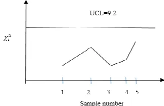
EPT=351; t1=3.3; UCL= 9.2; m=19; tm=14.38
This result indicates that monitoring of the process is started after passing 3.3 time unit from the start of each production cycle. Other inspection time points are obtained based on Equation (17). In each inspection time, a sample is taken from the process and for each item a vector of observation is obtained and the value of the statistic 𝜒𝑖2 is computed. The upper limit of the chi –
square control chart is 9.2. After passing 19 inspection periods and at time 14.38 the production cycle is terminated. Applying these approach leads to maximize the expected profit per time that is equal to 351. The control chart used in this example is illustrated in Figure 1.
Example 2. Suppose that the observation vector has three dimensions. The means of the process in the in-control state and out-of-in-control state are: 𝝁𝟎=
[1.5, 2.3, 2.5]; 𝝁𝟏′ = [4.7, 4.3, 6.6] respectively. The
covariance matrix is: Σ = [2.83 2.56.1 −14 4.2 3.8 5.1 ].
Figure 1. A Chi-square control chart to monitor the process
Based on equation 𝛿 = 𝑛(𝝁𝟏− 𝝁𝟎)′𝚺𝟎−𝟏(𝝁𝟏− 𝝁𝟎), 𝜹 =
𝟑. 𝟐𝟗. The other parameters are similar to Example 1. The results are as follows:
𝐸𝑃𝑇 =97.79; 𝑡1= 6.9; 𝑈𝐶𝐿 = 4.6; 𝑚 = 3; 𝑡𝑚= 11.95.
6. SENSETIVITY ANALYSIS
In this section, some sensitivity analysis is conducted on the key parameters of the process. Throughout this section, with respect to Example 1 in Section 5, some changes are made on the values of the process parameters and the result of the integrated model optimization is analyzed.
6. 1. The Effect of the Parameters of the Weibull Distribution In this subsection, the effect of the parameters of the Weibull distribution is studied. First, the effect of the shape parameter, 𝜈, is studied. Figure 2 illustrates the effect of the shape parameter. As can be seen, an increase in the value of the shape parameter has an increasing effect on the values of EPT and 𝑡1. On the
other hand, the increase in the value of the shape parameter leads to a decrease in the values of m and tm.
Increase in the value of 𝑡1 can be justified based on the
fact that in a Weibull distribution (for a fixed value of the scale parameter), increase of the shape parameter leads to the reduction of the variance of the distribution. Hence, for the larger values of the shape parameter, it is easier to predict the failure time. Also, change on the value of the shape parameter has no significant effect on the value of
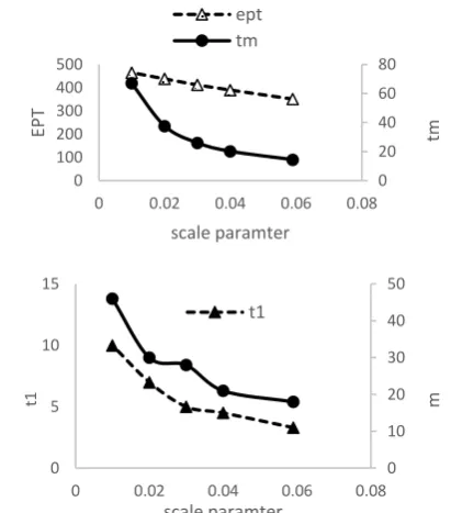
UCL. Now, we proceed to study the effect of the scale parameter of the Weibull distribution. The result is indicated in Figure 3.
TABLE 2. The parameters of the numerical example
parameter δ Cf Cv RI R0 C1 CCM CPM ZI ZRM ZPM 𝒗 = 𝒗𝟎= 𝒗𝟏 𝝀 = 𝝀𝟎 𝝀𝟏
Figure 2. the effect of the shape parameter of the Weibull distribution
Decreasing the values of the scale parameter, as expected, leads to an increase in the value of EPT, because in a Weibull distribution, the smaller values of the scale parameter yield to a larger values of the mean value.
Figure 3. The effect of the scale paramter of the Weibull
distribution
6. 2. The Effect of the Revenue Parameters In this subsection, the effect of change on the values of 𝑅0 and
𝑅1 is analyzed. First, assume that the values of 𝑅1
increases from 50 to 100. The results of optimization are as follows: EPT=352; t1=3.5; UCL=9.2; m=17; tm=14.3.
As observed, increase in the value of R1 from 50 to 100 does not have a significant effect on the decision variables of the model. In the next step, the values of R_0 changes from 500 to 200. The results are as follows: EPT=101; t1=4.9; UCL=7.8; m=10; tm=14.7
As can be seen, unlike the effect of R_1, a decrease in the value of R0 has a drastic decreasing effect on EPT , so that the value of EPT decreases from 351 to 101.
6. 3. The Effect of the Parameters of the Maintenance Costs Figure 4 illustrates the effect of the maintenance cost. To this end, the values of the corrective maintenance cost,𝐶𝐶𝑀 is increased, while the
preventive maintenance cost is unchanged. As expected, the increase in the value of 𝐶𝐶𝑀 leads to a decrease on
the value of EPT. Also, this change has a decreasing effect on the values of 𝑡𝑚 and m, while it has no
significant effect on the values of UCL and 𝑡1.
Figure 4. the effect of the values of the corrective
maintenance cost
4. CONCLOSION
In this paper, an integrated model for CBM and SPC is developed. With respect to the current CBM models that have used the multivariate control charts as a condition 0
5 10 15 20
340 350 360 370 380 390
2 2.5 3 3.5 4
tm
EPT
shape paramter (v) EPT tm
0 5 10 15 20
0 2 4 6 8
2 2.5 3 3.5 4
m
t1
shape paramter (v) t1 m
0 20 40 60 80
0 100 200 300 400 500
0 0.02 0.04 0.06 0.08
tm
EPT
scale paramter ept tm
0 10 20 30 40 50
0 5 10 15
0 0.02 0.04 0.06 0.08
m
t1
scale paramter t1
0 5 10 15 20 25
300 320 340 360 380
0 500 1000 1500 2000 2500
tm
EPT
Corrective maintenance cost
EPT tm
0 5 10 15 20 25
300 320 340 360 380
0 500 1000 1500 2000 2500
tm
EPT
Corrective maintenance cost
monitoring technique, the proposed model has a more general structure and a wider application domain because this model has three main novelties:
1- we place no restrictive assumption on the deterioration mechanism of the system. In other words, the time to quality shift as well as the time to the failure state from each operational states are assumed as a general continuous distribution function;
2- developing the integrated CBM and SPC model in this paper is based on the recursive equations and renewal reward process. Thus, the model can be easily applied for the other control charts; 3- the model can be applied for different types of inspection policy, because the inspection time points are considered as the decision variables of the model.
5. REFERENCES
1. Wu, J. and Makis, V., "Economic and economic-statistical design of a chi-square chart for cbm", European Journal of operational research, Vol. 188, No. 2, (2008), 516-529.
2. Wang, W., "A simulation-based multivariate bayesian control chart for real time condition-based maintenance of complex systems", European Journal of Operational Research, Vol. 218, No. 3, (2012), 726-734.
3. Liu, L., Yu, M., Ma, Y. and Tu, Y., "Economic and economic-statistical designs of an x control chart for two-unit series systems with condition-based maintenance", European Journal of Operational Research, Vol. 226, No. 3, (2013), 491-499.
4. Mishra, A. and Jain, M., "Maintainability policy for deteriorating system with inspection and common cause failure", Int J Eng Trans C Basics, Vol. 26, No. 6, (2013), 371-380.
5. Rabani, M., Manavizadeh, N. and Balali, S., "A stochastic model for indirect condition monitoring using proportional covariate model", Vol. 21, (2008), 45-56.
6. Panagiotidou, S. and Tagaras, G., "Statistical process control and condition‐based maintenance: A meaningful relationship through data sharing", Production and Operations Management, Vol. 19, No. 2, (2010), 156-171.
7. Mehrafrooz, Z. and Noorossana, R., "An integrated model based on statistical process control and maintenance", Computers & Industrial Engineering, Vol. 61, No. 4, (2011), 1245-1255. 8. Xiang, Y., "Joint optimization of x¯ control chart and preventive
maintenance policies: A discrete-time markov chain approach", European Journal of Operational Research, Vol. 229, No. 2, (2013), 382-390.
9. Panagiotidou, S. and Tagaras, G., "Optimal integrated process control and maintenance under general deterioration", Reliability Engineering & System Safety, Vol. 104, (2012), 58-70. 10. Yin, H., Zhang, G., Zhu, H., Deng, Y. and He, F., "An integrated
model of statistical process control and maintenance based on the delayed monitoring", Reliability Engineering & System Safety, Vol. 133, (2015), 323-333.
11. Panagiotidou, S. and Nenes, G., "An economically designed, integrated quality and maintenance model using an adaptive shewhart chart", Reliability Engineering & System Safety, Vol. 94, No. 3, (2009), 732-741.
12. Ardakan, M.A., Hamadani, A.Z., Sima, M. and Reihaneh, M., "A hybrid model for economic design of mewma control chart under maintenance policies", The International Journal of Advanced Manufacturing Technology, Vol. 83, No. 9-12, (2016), 2101-2110.
13. Jamshidi, R. and Maadi, M., "Maintenance and work-rest scheduling in human-machine system according to fatigue and reliability", International Journal of Engineering, Vol. 30, No. 1, (2017), 85-92.
14. Liu, L., Jiang, L. and Zhang, D., "An integrated model of statistical process control and condition-based maintenance for deteriorating systems", Journal of the Operational Research Society, Vol. 68, No. 11, (2017), 1452-1460.
15. Munford, A., "Comparison among certain inspection policies", Management Science, Vol. 27, No. 3, (1981), 260-267.
Application of Multivariate Control Charts for Condition Based Maintenance
H. Rasay, M.S. Fallahnezhad, Y.Zaremehrjerdi
Department of Industrial Engineering, Yazd University, Yazd, Iran
P A P E R I N F O
Paper history:
Received 28 May 2017
Received in revised form 26 September 2017 Accepted 12 October 2017
Keywords: Condition Monitoring Condition Based Maintenance Statistical Process Control Multivariate Control Chart
هديكچ
هدمآ تسدب تاعلاطا نداد طابترا یارب لاومعم .تسا تیعضو شیاپ ،تیعضو رب ینتبم تاریمعت و یرادهگن تسایس ساسا هک یکیدزن طابترا نتفگ رظنرد اب ،رگید فرط زا .تسا یلامتحا یاه لدم هب زاین ،متسیس یعقاو تلاح هب تیعضو شیاپ زا لرتنک و تیعضو رب ینتبم تاریمعت و یرادهگن نیب .تسا هدش هداد هعسوت هچراپکی یاه لدم ،دراد دوجو یرامآ دنیارف
یتایلمع تیعضو دروم رد طابنتسا و دننک یم هدافتسا تیعضو شیاپ رازبا کی ناونع هب لرتنک یاهرادومن زا اه لدم نیا ک دوش یم هتفرگ میمصت تیاهنرد .دریگ یم تروص تیعضو شیاپ زا هدمآ تسدب تاعلاطا یانبمرب متسیس ریبادت عون هچ ه
،تیعضو شیاپ کینکت کی ناونع هب ار هریغتم دنچ لرتنک یاهرادومن دربراک هلاقم نیا .دوش هتفگراک هب یتاریمعت و یرادهگن زا هکیلاح رد هدش هداد هعسوت هچراپکی لدم کی ،اتسار نیا رد .دهد یم ناشن تیعضو رب ینتبم تاریمعت و یرادهگن رد اوکسا یاک لرتنک رادومن تسایس ناونع تحت تسایس کی ،یسرزاب یاه هرود نییعت یارب نینچمه .دوش یم هدافتسا ر
خرن
یم هتفرگ راک هب تباث یبارخ دوش
.