J.-S. Dhersin, Editor
CONVERGENCE RESULTS ON GREEDY ALGORITHMS FOR
HIGH-DIMENSIONAL EIGENVALUE PROBLEMS
∗Virginie Ehrlacher
1Abstract. In this paper, we present two greedy algorithms for the computation of the lowest eigen-value (and an associated eigenvector) of a high-dimensional eigeneigen-value problem, which have been intro-duced and analyzed recently in a joint work with Eric Cancès and Tony Lelièvre [1]. The performance of our algorithms is illustrated on toy numerical test cases, and compared with that of another greedy algorithm for eigenvalue problems introduced by Ammar and Chinesta [13].
Résumé. Dans ce document, nous présentons deux algorithmes gloutons for le calcul de la plus petite valeur propre (et d’un vecteur propre associé) d’un problème aux valeurs propres en grande dimension, qui ont été récemment introduits et analysés dans un travail commun avec Eric Cancès et Tony Lelièvre [1]. Le comportement numérique de ces algorithmes est illustré sur de petits cas tests, et comparé à celui d’un autre algorithme glouton proposé antérieurement par Ammar et Chinesta [13].
Introduction
High dimensional problems are encountered in many application fields, among which electronic structure calculations, molecular dynamics, uncertainty quantification, multiscale homogenization, and mathematical finance. The numerical simulation of these problems, which requires specific approaches due to the so-called
curse of dimensionality [2], has fostered the development of a wide variety of new numerical methods and algorithms, such as sparse grids [3, 4], reduced bases [5], sparse tensor products [6], and adaptive polynomial approximations [7].
In this article, we focus on an approach introduced by Ladevèze [8], Chinesta [9], Nouy [10] and coauthors in different contexts, relying on the use of greedy algorithms[11]. This class of methods is also calledProgressive Generalized Decomposition[12] in the literature.
The idea of these methods consist in approximating a functionu(x1,· · ·, xd) depending on a possibly very
large number of variablesx1,· · ·, xd as a sum of so-calledtensor productfunctions,
u(x1,· · ·, xd)≈
X
k≥1
rk(1)(x1)· · ·r(kd)(xd),
where each of these tensor product functions appearing in the above sum is computed in an iterative way asthe best next tensor product in a sense which depends on the nature of the problemuis solution of.
∗This work has been done while the author was a long-term visitor at IPAM (UCLA).
1 Université Paris Est, CERMICS, Projet MICMAC, Ecole des Ponts ParisTech - INRIA, 6 & 8 avenue Blaise Pascal, 77455
Marne-la-Vallée Cedex 2, France; e-mail:[email protected]
c
EDP Sciences, SMAI 2014
Greedy algorithms have been extensively studied in the framework of convex unconstrained minimization problems, in other words whenuis the solution of a problem of the form
u=argmin
v∈V
E(v), (1)
where V is a Hilbert space of functions depending on the d variables x1,· · ·, xd, and E is a convex energy
functional [14–16]. However, the analysis of such algorithms for other kinds of problems is less advanced [12]. We refer to [17] for a review of the mathematical issues arising in the application of greedy algorithms to non-symmetric linear problems. To our knowledge, the literature on greedy algorithms for eigenvalue problems is very limited. Penalized formulations of constrained minimization problems enable one to recover the structure of unconstrained minimization problems and to benefit from the sound theoretical framework existing in this case [14, 22]. The only reference we are aware of about greedy algorithms for eigenvalue problems without the use of a penalized formulation is an article by Ammar and Chinesta [13], in which the authors propose a greedy algorithm to compute the lowest eigenstate of a bounded from below self-adjoint operator, and apply it to electronic structure calculation. No analysis for this algorithm is given though.
In this paper, we present two new greedy algorithms for the computation of the lowest eigenstate of high-dimensional eigenvalue problems which were introduced and analyzed recently in [1]. We present the main theoretical results proved in the latter paper and illustrate the numerical behaviour of the algorithms on some toy numerical test cases. The outline of the paper is the following: we first introduce some notation and assumptions in Section 1; the description of the greedy algorithms and the associated theoretical convergence results are detailed in Section 2. We refer the reader to [1] for the detailed proofs of these results and an exhaustive description of the implementation of these algorithms in practice. The last section 3 contains some toy numerical tests for illustration.
1.
Preliminaries
1.1.
Notation and main assumptions
Let us consider two Hilbert spacesV andH, endowed respectively with the scalar productsh·,·iV andh·,·i,
such that, unless it is otherwise stated,
(HV) the embeddingV ֒→H is dense and compact.
The associated norms are denoted respectively byk · kV and k · k. Let us recall that it follows from (HV) that
the weak convergence inV implies the strong convergence in H.
Leta:V ×V →Rbe a symmetric continuous bilinear form onV ×V such that
(HA) ∃γ, ν >0, such that ∀v∈V, a(v, v)≥γkvk2
V −νkvk2.
The bilinear formh·,·ia, defined by
∀v, w∈V, hv, wia:=a(v, w) +νhv, wi, (2)
is a scalar product on V, whose associated norm, denoted byk · ka, is equivalent to the normk · kV. Besides,
we can also assume without loss of generality that the constantν is chosen so that for allv∈V,kvka≥ kvk.
It is well-known (see e.g. [18]) that, under the above assumptions (namely (HA) and (HV)), there exists a sequence(ψp, µp)p∈N∗ of solutions to the elliptic eigenvalue problem
find(ψ, µ)∈V ×Rsuch thatkψk= 1and
∀v∈V, a(ψ, v) =µhψ, vi (3)
In the case when the embedding V ֒→ H is dense but not compact (i.e. when (HV) does not hold), the spectrum of the unique self-adjoint operator A onH with form domainV associated with the quadratic form
a(·,·) can be purely continuous; in this case, (3) has no solution. However, if A has at least one discrete eigenvalue located below the minimum of its essential spectrum, convergence results for the second algorithm we propose can be established. This is the object of Proposition 2.1.
Definition 1.1. A setΣ⊂V is called a dictionaryofV ifΣsatisfies the following three conditions:
(HΣ1): Σis a non-empty cone, i.e. 0∈Σand for all(z, t)∈Σ×R,tz∈Σ;
(HΣ2): Σis weakly closed inV;
(HΣ3): Span(Σ) is dense inV.
In practical applications for high-dimensional eigenvalue problems, the setΣis typically an appropriate set of tensor formats used to perform the greedy algorithms presented in Section 2.1. We also denote by
Σ∗:= Σ\ {0}. (4)
1.2.
Prototypical example
Let us present a prototypical example of the high-dimensional eigenvalue problems we have in mind, along with possible dictionaries.
LetX1, . . . , Xdbe bounded regular domains ofRm1, . . . , Rmdrespectively. LetV =H01(X1× · · · × Xd)and
H =L2(X
1× · · · × Xd). It follows from the Rellich-Kondrachov theorem that these spaces satisfy assumption
(HV). Letb:X1× · · · × Xd→Rbe a measurable real-valued function such that
∃β, B >0, such that β≤b(x1, . . . , xd)≤B, for a.e. (x1, . . . , xd)∈ X1× · · · × Xd.
Besides, letW ∈Lq(X
1× · · · × Xd)withq= 2ifm≤3, andq > m/2 form≥4wherem:=m1+· · ·+md. A
prototypical example of a continuous symmetric bilinear forma:V ×V →Rsatisfying (HA) is
∀v, w∈V, a(v, w) :=
Z
X1×···×Xd
(b∇v· ∇w+W vw). (5)
In this particular case, the eigenvalue problem (3) also reads
find(ψ, µ)∈H1
0(X1× · · · × Xd)×Rsuch thatkψkL2(X1×···×X
d)= 1and
−div(b∇ψ) +W ψ=µψin D′(X
1× · · · × Xd).
For all 1 ≤j ≤d, we denote byVj :=H01(Xj). Some examples of dictionariesΣ based on different tensor
formats satisfying (HΣ1), (HΣ2) and (HΣ3) are the set of rank-1 tensor-product functions
Σ⊗ :=nr(1)⊗ · · · ⊗r(d)| ∀1≤j ≤d, r(j)∈Vj
o
, (6)
as well as other tensor formats [6, 19], for instance the sets of rank-R Tucker, rank-R Tensor Train, or rank-R
Tensor Chain functions, withR∈N∗.
2.
Greedy algorithms for eigenvalue problems
In the rest of the paper, we present two different greedy algorithms to compute an eigenpair associated to the lowest eigenvalue of the elliptic eigenvalue problem (3).
Section 2.2 contains our main convergence results. The choice of a good initial guess for all these algorithms is discussed in [1] and is not detailed here for the sake of brevity. For a detailed proof of the results stated in this section, we refer the reader to [1].
For allv∈V, we denote by
J(v) :=
( a(v,v)
kvk2 ifv6= 0, +∞ ifv= 0,
the Rayleigh quotient associated to (3), and
λΣ:= inf
z∈ΣJ(z) = infz∈Σ∗
a(z, z) kzk2 .
Note that, sinceΣ⊂V,λΣ≥µ1= inf v∈VJ(v).
2.1.
Description of the algorithms
2.1.1. Pure Rayleigh Greedy Algorithm
The following algorithm, called hereafter thePure Rayleigh Greedy Algorithm(PRaGA) algorithm, is inspired from the Pure Greegy Algorithm for convex minimization problems (see [14, 15] for instance).
Pure Rayleigh Greedy Algorithm (PRaGA):
• Initialization: choose an initial guess u0∈V such thatku0k= 1and such thatλ0:=a(u0, u0)< λΣ;
• Iterate on n≥1: findzn ∈Σsuch that
zn∈argmin z∈Σ
J(un−1+z), (7)
and set un:= kunun−1+zn
−1+znk andλn:=a(un, un).
The choice of an initial guessu0∈V satisfyingku0k= 1anda(u0, u0)≤λΣ is discussed [1].
The following lemma holds, stating that the iterations of the PRaGA are well-defined:
Lemma 2.1. LetV andH be separable Hilbert spaces satisfying (HV),Σa dictionary ofV anda:V×V →R
a symmetric continuous bilinear form satisfying (HA). Then, all the iterations of the PRaGA algorithm are well-defined in the sense that for alln∈N∗, there exists at least one solution to the minimization problem (7).
Besides, the sequence(λn)n∈N∗ is non-increasing.
2.1.2. Pure Residual Greedy Algorithm
ThePure Residual Greedy Algorithm(PReGA) we propose is based on the use of a residual for problem (3). Pure Residual Greedy Algorithm (PReGA):
• Initialization: choose an initial guess u0∈V such thatku0k= 1and letλ0:=a(u0, u0);
• Iterate on n≥1: findzn ∈Σsuch that
zn∈argmin z∈Σ
1
2kun−1+zk
2
a−(λn−1+ν)hun−1, zi, (8)
and set un:= kunun−1+zn
−1+znk andλn:=a(un, un).
The denominationResidualcan be justified as follows: it is easy to check that for alln∈N∗, the minimization
problem (8) is equivalent to the minimization problem
findzn∈Σsuch thatzn ∈argmin z∈Σ
1
2kRn−1−zk
2
where Rn−1∈V is the Riesz representant inV of the linear formln−1:v ∈V 7→λn−1hun−1, vi −a(un−1, v). In other words,Rn−1 is the unique element inV such that
∀v∈V, hRn−1, via=λn−1hun−1, vi −a(un−1, v).
The linear formln−1 can indeed be seen as a residual for (3) sinceln−1= 0if and only ifλn−1is an eigenvalue ofa(·,·)andun−1 an associatedH-normalized eigenvector.
Let us point out that, in order to carry out the PReGA in practice, one needs to know the value of a constant
ν ensuring (HA), whereas this is not needed for the PRaGA, neither for the algorithm (PEGA) introduced in [13] and considered in the next section.
Lemma 2.2. LetV andH be separable Hilbert spaces such that the embeddingV ֒→H is dense,Σa dictionary of V and a : V ×V → R a symmetric continuous bilinear form satisfying (HA). Then, all the iterations of
the PReGA algorithm are well-defined in the sense that for all n∈N∗, there exists at least one solution to the
minimization problem (8).
2.1.3. Pure Explicit Greedy Algorithm
The above two algorithms are new, at least to our knowledge. In this section, we describe the algorithm already proposed in [13], which we call in the rest of the paper thePure Explicit Greedy Algorithm (PEGA).
Unlike the above two algorithms, the PEGA is not defined for general dictionariesΣsatisfying (HΣ1), (HΣ2) and (HΣ3). We need to assume in addition thatΣis an embedded manifold in V. In this case, for allz∈Σ, we denote byTΣ(z)the tangent subspace toΣat the pointzin V.
Let us point out that, ifΣis an embedded manifold inV, for all n∈N∗, the Euler equations associated to
the minimization problems (7) and (8) respectively read:
∀δz∈TΣ(zn), a(un−1+zn, δz) =λnhun−1+zn, δzi, (10)
and
∀δz∈TΣ(zn), a(un−1+zn, δz) +νhzn, δzi=λn−1hun−1, δzi. (11)
The PEGA consists in solving at each iterationn∈N∗of the greedy algorithm the following equation, which
is of a similar form as the Euler equations (10) and (11) above,
∀δz∈TΣ(zn), a(un−1+zn, δz) =λn−1hun−1+zn, δzi. (12)
More precisely, the PEGA algorithm reads:
Pure Explicit Greedy Algorithm (PEGA):
• Initialization: choose an initial guess u0∈V such thatku0k= 1and letλ0:=a(u0, u0);
• Iterate for n≥1: findzn∈Σsuch that
∀δz∈TΣ(zn), a(un−1+zn, δz)−λn−1hun−1+zn, δzi= 0, (13)
and set un:= kunun−−11++znznk andλn:=a(un, un).
Notice that (13) is very similar to (10) except that λn−1 is used instead ofλn. It can be seen as anexplicit
version of the PRaGA, hence the namePure Explicit Greedy Algorithm .
Note that it is not clear whether there always exists a solution zn to (13), since (13) does not derive from
2.1.4. Orthogonal algorithms
We introduce here slightly modified versions of the PRaGA, PReGA and PEGA, inspired from theOrthogonal Greedy Algorithm for convex minimization problems (see for instance [15, 16]).
Orthogonal (Rayleigh, Residual or Explicit) Greedy Algorithm (ORaGA, OReGA and OEGA):
• Initialization: choose an initial guessu0 ∈ V such that ku0k = 1 and let λ0 := a(u0, u0). For the ORaGA, we need to assume thatλ0:=a(u0, u0)< λΣ.
• Iterate on n≥1:
– for the ORaGA: findzn ∈Σsatisfying (7);
– for the OReGA: findzn ∈Σsatisfying (8);
– for the OEGA: findzn∈Σsatisfying (13);
findc(0n), . . . , c (n) n
∈Rn+1 such that
c(0n), . . . , c(nn)
∈ argmin
(c0,...,cn)∈Rn+1
J (c0u0+c1z1+· · ·+cnzn), (14)
and set un:= c
(n)
0 u0+c(1n)z1+···+c(nn)zn
kc(0n)u0+c1(n)z1+···+c(nn)znk
; ifhun−1, uni ≤0, set un :=−un; setλn:=a(un, un).
Let us point out that the original algorithm proposed in [13] is the OEGA. Besides, for the three algorithms and alln∈N∗, there always exists at least one solution to the minimization problems (14).
For the sake of brevity, we do not detail here how the problems (7), (8) and (13) are solved in practice and refer the reader to [1] for further details in the case when the dictionary Σis the set of rank-1 tensor product functions.
The orthogonal versions of the greedy algorithms can be easily implemented from the pure versions: at any iterationn∈N∗, only an additional step is performed, which consists in choosing an approximate eigenvectorun
as a linear combination of the elementsu0, z1, . . . , znminimizing the Rayleigh quotient associated to the bilinear
form a(·,·). Sinceun is called to be the approximation of an eigenvector associated to the lowest eigenvalue of
a(·,·), which is a minimizer of the Rayleigh quotient on the Hilbert spaceV, this additional step is a natural extension of the Orthogonal Greedy Algorithm for the minimization of convex energy functionals [15].
2.2.
Convergence results
2.2.1. The infinite-dimensional case
Theorem 2.1. LetV andH be separable Hilbert spaces satisfying (HV),Σa dictionary ofV anda:V×V →R
a symmetric continuous bilinear form satisfying (HA). The following properties hold for the PRaGA, ORaGA, PReGA and OReGA:
(1) All the iterations of the algorithms are well-defined.
(2) The sequence(λn)n∈Nis non-increasing and converges towards a limitλwhich is an eigenvalue ofa(·,·) for the scalar product h·,·i.
(3) The sequence (un)n∈N is bounded in V and any subsequence of (un)n∈N which weakly converges in V also strongly converges in V towards an H-normalized eigenvector associated with λ. This implies in particular that
da(un, Fλ) := inf
w∈Fλkw−unkan−→→∞0,
whereFλ denotes the set of theH-normalized eigenvectors of a(·,·)associated with λ.
(4) If λ is a simple eigenvalue, then there exists an H-normalized eigenvector wλ associated with λ such
that the whole sequence(un)n∈N converges towλ strongly in V.
It may happen that λ > µ1, if the initial guess u0 is not properly chosen. This point is discussed in more details in [1]. If λ is degenerate, it is not clear whether the whole sequence (un)n∈N converges. We will see
(un)n∈N always converges towards an element wλ ∈ V which is an eigenvector of a(·,·) associated with λ.
However, λmay still be strictly greater than µ1, even in this case. However, if the initial guess u0 is chosen such thatλ0 is strictly lower any eigenvalue ofa(·,·)exceptµ1, then(λn)n∈Nnecessarily converges toµ1.
In addition, for the PReGA and the OReGA, we can prove similar convergence results without assuming that the Hilbert spaceV is compactly embedded inH, provided that the self-adjoint operatorAassociated with the quadratic forma(·,·)has at least one eigenvalue below the minimum of its essential spectrum.
Proposition 2.1. Let V andH be separable Hilbert spaces such that the embedding V ֒→H is dense (but not necessarily compact),Σa dictionary ofV,a:V×V →Ra symmetric continuous bilinear form satisfying (HA),
andAthe self-adjoint operator onHassociated toa(·,·). Let us assume also thatminσ(A)<minσess(A), where
σ(A)andσess(A)respectively denote the spectrum and the essential spectrum of A, and that the initial guessu0
satisfiesminσ(A)≤λ0:=a(u0, u0)<minσess(A). Then, the following properties hold for the PReGA and the
OReGA:
(1) All the iterations of the algorithms are well-defined.
(2) The sequence(λn)n∈Nis non-increasing and converges towards a limitλwhich is an eigenvalue ofa(·,·) for the scalar product h·,·i such thatλ <minσess(A).
(3) The sequence (un)n∈N is bounded in V and any subsequence of (un)n∈N which weakly converges in V also strongly converges in V towards an H-normalized eigenvector associated with λ. This implies in particular that
da(un, Fλ) := inf
w∈Fλkw−unkan−→→∞0,
whereFλ denotes the set of H-normalized eigenvectors of a(·,·) associated withλ.
(4) If λ is a simple eigenvalue, then there exists an H-normalized eigenvector wλ associated with λ such
that the whole sequence(un)n∈N converges towλ strongly in V.
2.2.2. The finite-dimensional case
From now on, for any differentiable functionf :V →R, and allv0∈V, we denote by f′(v0)the derivative
of the function f at the pointv0 ∈V. More precisely, f′(v0)∈V′ is the unique continuous linear form on V such that for allv∈V,
f(v) =f(v0) +hf′(v0), v−v0iV′,V +r(v), with lim kvka→0
r(v) kvka
= 0.
Besides, we define the injective norm onV′ associated toΣas follows:
∀l∈V′, klk∗ = sup
z∈Σ∗
hl, ziV′,V
kzka
.
In the rest of this section, we assume that V, hence H (since the embedding V ֒→ H is dense), are finite dimensional vector spaces. The convergence results below heavily rely on the Łojasiewicz inequality [20] and the ideas presented in [21] for the proof of convergence of gradient-based algorithms for the Hartree-Fock equations.
The Łojasiewicz inequality [20] reads as follows:
Lemma 2.3. LetΩbe an open subset of the finite-dimensional Euclidean spaceV, andf an analytic real-valued function defined on Ω. Then, for eachv0∈Ω, there is a neighborhood U ⊂Ω ofv0 and two constants K∈R+
andθ∈(0,1/2]such that for allv∈U,
|f(v)−f(v0)|1−θ≤Kkf′(v)k∗. (15)
is easy to see thatθ can be chosen to be equal to 1
2 by using a simple Taylor expansion. Moreover, whenv0 is a degenerate critical point of f, the analyticity assumption ensures that there existsN ∈N∗ such that the
Nth-order derivatives cannot vanish simultaneously, and the exponentθ can be chosen to be equal to 1 N.
In our context, the following lemma can be proved [1].
Lemma 2.4. Let V andH be finite-dimensional Euclidean spaces,Ω :={v ∈V, 1/2 <kvk<3/2},λ be an eigenvalue of the bilinear forma(·,·)andFλ be the set of the H-normalized eigenvectors of a(·,·) associated to
λ. Then,J : Ω→Ris analytic, and there exists K∈R+,θ∈(0,1/2]andε >0 such that
for allv∈Ωsuch that d(v, Fλ) := inf
w∈Fλkv−wk ≤ε, |J(v)−λ| 1−θ
≤KkJ′(v)k∗. (16)
Using this lemma, the following convergence rates in finite dimension can be obtained:
Theorem 2.2. LetV andH be finite dimensional Euclidian spaces anda:V ×V →Rbe a symmetric bilinear
form. The following properties hold for both PRaGA and PReGA:
(1) the whole sequence (un)n∈Nstrongly converges inV to somewλ∈Fλ;
(2) the convergence rates are as follows, depending on the value of the parameter θ in (16): • ifθ= 1/2, there existsC∈R+ and0< σ <1such that for all n∈N,
kun−wλka≤Cσn; (17)
• ifθ∈(0,1/2), there existsC∈R+ such that for all n∈N∗,
kun−wλka ≤Cn− θ
1−2θ. (18)
3.
Numerical results
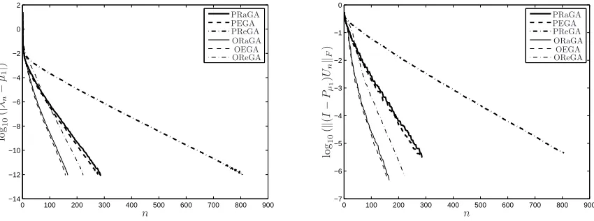
We present here some numerical results obtained with these algorithms (PRaGA, PReGA, PEGA and their orthogonal versions) on toy examples involving only two Hilbert spaces (d = 2). We refer the reader to [13] for numerical examples involving a larger number of variables. These basic numerical tests performed with small-dimensional matrices lead us to think that the greedy algorithms presented above converge in general towards the lowest eigenvalue of the bilinear form under consideration, except in pathological situations which are not likely to be encountered in practice.
In this simple example, we take V =H =RNx×Ny,Vx =RNx and Vy =RNy for some Nx, Ny ∈N∗ (here
typically Nx=Ny = 51). Let D1x, D2x ∈RNx×Nx and D1y, D2y ∈RNy×Ny be (randomly chosen) symmetric
definite positive matrices. We aim at computing the lowest eigenstate of the symmetric bilinear form
a(U, V) =Tr UT(D1xV D1y+D2xV D2y)
,
or, in other words, of the symmetric fourth order tensorAdefined by
∀1≤i, k≤Nx, 1≤j, l≤Ny, Aij,kl=D1ikxD 1y jl +D
2x ikD
2y jl.
Let us denote byµ1the lowest eigenvalue of the tensorA, byIthe identity operator, and byPµ1 ∈ L(R
Nx×Ny)
the orthogonal projector onto the eigenspace ofAassociated withµ1. Figure 1 shows the decay of the error on the eigenvalueslog10(|µ1−λn|)and of the error on the eigenvectorslog10(k(I−Pµ1)UnkF), wherek · kF denotes
the Frobenius norm ofRNx×Ny, as a function ofnfor the three algorithms and their orthogonal versions.
These tests were performed with several matricesD1x, D1y, D2x, D2y, either drawn randomly or chosen such
Besides, the rate of convergence always seems to be exponential with respect ton. The error on the eigenvalues decays twice as fast as the error on the eigenvectors, as usual when dealing with the approximation of linear eigenvalue problems.
We observe that the PRaGA and PEGA have similar convergence properties with respect to the number of iterationsn. The behaviour of the PReGA strongly depends on the value ν chosen in (HA): the largerν, the slower the convergence of the PReGA. To ensure the efficiency of this method, it is important to choose the numerical parameter ν ∈ R appearing in (2) as small as possible so that (HA) remains true. If the value of
ν is well-chosen, the PReGA may converge as fast as the PRaGA or the PEGA. In the example presented in Figure 1 whereν is chosen to be0andµ1≈116, we can clearly see that the rate of convergence of the PReGA is poorer than the rates of the PRaGA and PEGA.
We also observe that the use of the ORaGA, OReGA and OEGA, instead of the pure versions of the algorithms, improves the convergence rate with respect to the number of iterations n ∈ N∗. However, as n
increases, the cost of then-dimensional optimization problems (14) becomes more and more significant.
0 100 200 300 400 500 600 700 800 900 −14 −12 −10 −8 −6 −4 −2 0 2 OEGA PEGA OReGA PReGA ORaGA PRaGA lo
g10
( | λn − µ1 | )
n 0 100 200 300 400 500 600 700 800 900
−7 −6 −5 −4 −3 −2 −1 0 OEGA PEGA OReGA PReGA ORaGA PRaGA lo
g10
( k ( I − Pµ 1 ) Un kF ) n
Figure 1. Decay of the error of the three algorithms and their orthogonal versions: eigenvalues
(left) and eigenvectors (right).
References
[1] E. Cancès, V. Ehrlacher and T. Lelièvre, Greedy algorithms for high-dimensional eigenvalue problems, http://arxiv.org/abs/1304.2631 (2013).
[2] R.E. Bellman,Dynamic Programming, Princeton University Press, 1957. [3] H. Bungartz and M. Griebel,Sparse grids, Acta Numerica 13 (2004) 147–269.
[4] T. von Petersdorff and C. Schwab,Numerical solution of parabolic equations in high dimensions, M2AN Mathematical Mod-elling and Numerical Analysis 38 (2004) 93–127.
[5] A. Buffa, Y. Maday, A.T. Patera, C. Prud’homme and G. Turinici,A priori convergence of the greedy algorithm for the parametrized reduced basis, ESAIM: Mathematical Modelling and Numerical Analysis 46 (2012) 595–603.
[6] W. Hackbusch,Tensor spaces and numerical tensor calculus, Springer, 2012.
[7] A. Chkifa, A. Cohen, R. DeVore and C. Schwab,Sparse adaptive Taylor approximation algorithms for parametric and stochastic elliptic PDEs, ESAIM: Mathematical Modelling and Numerical Analysis 47 (2013) 253–280.
[8] P. Ladevèze, Nonlinear computational structural mechanics: new approaches and non-incremental methods of calculation, Springer (Berlin), 1999.
[9] A. Ammar, B. Mokdad, F. Chinesta and R. Keunings,A new family of solvers for some classes of multidimensional partial differential equations encountered in kinetic theory modeling of complex fluids, Journal of Non-Newtonian Fluid Mechanics 139 (2006) 153–176.
[11] V.N. Temlyakov,Greedy Approximation, Acta Numerica 17 (2008) 235–409.
[12] F. Chinesta, P. Ladevèze and E. Cueto,A short review on model order reduction based on Proper Generalized Decomposition, Archives of Computational Methods in Engineering 18 (2011) 395–404.
[13] A. Ammar and F. Chinesta, Circumventing the curse of dimensionality in the solution of highly multidimensional models encountered in Quantum Mechanics using meshfree finite sums decompositions, Lecture notes in Computational Science and Engineering 65 (2008) 1–17.
[14] E. Cancès, V. Ehrlacher and T. Lelièvre, Convergence of a greedy algorithm for high-dimensional convex problems, Mathe-matical Models and Methods in Applied Sciences 21 (2011) 2433–2467.
[15] A. Nouy and A. Falco,Proper Generalized Decomposition for nonlinear convex problems in tensor Banach spaces, Numerische Mathematik 121 (2012) 503–530.
[16] C. Le Bris, T. Lelièvre and Y. Maday, Results and questions on a nonlinear approximation approach for solving high-dimensional partial differential equations, Constructive Approximation 30 (2009) 621–651.
[17] E. Cancès, V. Ehrlacher and T. Lelièvre, Greedy algorithms for high-dimensional non-symmetric linear problems, arXiv:1210.6688 (2012).
[18] M. Reed and B. Simon,Methods of Modern Mathematical Physics IV: Analysis of Operators, Academic Press, 1978. [19] V. Khoromskai, B.N. Khoromskij and R. Schneider,QTT representation of the Hartree and Exchange operators in electronic
structure calculations, Computational Methods in Applied Mathematics 11 (2011) 327–341. [20] S. Lojasiewicz,Ensembles semi-analytiques, Institut des Hautes Etudes Scientifiques, 1965.
[21] A. Levitt, Convergence of gradient-based algorithms for the Hartree-Fock equations, ESAIM: Mathematical Modelling and Numerical Analysis (M2AN) 46 (2012) 1321–1336.