N. Champagnat, T. Leli`evre, A. Nouy, Editors
TENSOR NUMERICAL METHODS FOR MULTIDIMENSIONAL PDES:
THEORETICAL ANALYSIS AND INITIAL APPLICATIONS
Boris N. Khoromskij
1Abstract. We present a brief survey on the modern tensor numerical methods for multidimen-sional stationary and time-dependent partial differential equations (PDEs). The guiding principle of the tensor approach is the rank-structured separable approximation of multivariate functions and operators represented on a grid. Recently, the traditional Tucker, canonical, and matrix product states (tensor train) tensor models have been applied to the grid-based electronic structure cal-culations, to parametric PDEs, and to dynamical equations arising in scientific computing. The essential progress is based on the quantics tensor approximation method proved to be capable to represent (approximate) function relatedd-dimensional data arrays of sizeNdwith log-volume com-plexity,O(dlogN). Combined with the traditional numerical schemes, these novel tools establish
a new promising approach for solving multidimensional integral and differential equations using low-parametric rank-structured tensor formats. As the main example, we describe the grid-based tensor numerical approach for solving the 3D nonlinear Hartree-Fock eigenvalue problem, that was the starting point for the developments of tensor-structured numerical methods for large-scale com-putations in solving real-life multidimensional problems. We also discuss a new method for the fast 3D lattice summation of electrostatic potentials by assembled low-rank tensor approximation capable to treat the potential sum over millions of atoms in few seconds. We address new results on tensor approximation of the dynamical Fokker-Planck and master equations in many dimensions up tod= 20. Numerical tests demonstrate the benefits of the rank-structured tensor approximation
on the aforementioned examples of multidimensional PDEs. In particular, the use of grid-based tensor representations in the reduced basis of atomics orbitals yields an accurate solution of the Hartree-Fock equation on largeN×N×N grids with a grid size of up toN= 105.
Introduction
In the recent years, the tensor numerical methods were recognized as the basic tool to render numerical simulations in higher dimensions tractable. The guiding principle of the tensor numerical methods is the reduction of the computational process onto a low parametric rank-structured manifold by using an approx-imation of multivariate functions and operators, that relies on a certain separation of variables. Possible applications of tensor numerical methods include high-dimensional problems arising in material- and bio-sciences, computational quantum chemistry, stochastic modeling and uncertainty quantification, dynamical systems, machine learning, financial mathematics, etc.
In the following discussion a tensor of orderd and mode sizeN, or briefly N-d tensor, is considered as a function on ad-fold product index set, A:I⊗d →Rwith I⊗d =I× · · · ×I, andI ={1, ..., N}. In the
traditional grid-based numerical techniques ford-dimensional PDEs the parameterN can be associated with the univariate grid size. The representation of arising N-d tensors (coefficient vectors) requires a storage size that is exponential in d, Nd, which causes severe computational difficulties, often called the “curse of
dimensionality“ [10].
1Max-Planck-Institute for Mathematics in the Sciences, Inselstr. 22-26, D-04103 Leipzig, Germany;
[email protected], http://personal-homepages.mis.mpg.de/bokh/.
c
EDP Sciences, SMAI 2015
A class of methods which lead to linear scaling in the dimension are distinctly linked with the principle of separation of variables. The multi-linear tensor decompositions based on the Tucker and canonical models have long since been used as a tool for data processing in the computer science community (e. g. PCA type methods), and applied to multidimensional experimental data in chemometrics, psychometrics and in signal processing, see a comprehensive bibliography in [84]. The remarkable approximating properties of the Tucker and canonical decomposition for wide classes of function related tensors were revealed in [65, 72], promoting its usage as a tool for the numerical treatment of multidimensional problems in numerical analysis. An introductory description of traditional tensor formats with the focus on tensor-structured numerical methods for the calculation of multidimensional functions and operators is presented in [55, 70, 71]. Moreover, the canonical tensor representations obtained by sinc approximations on a class of analytic multivariate functions have been proven to provide fast exponential convergence in the separation rank [34, 44, 65, 126].
First successes in the rank-structured tensor calculations of multivariate functions and operators in the Hartree-Fock equation originated the grid-based tensor numerical methods in scientific computing [55, 58, 60–62, 73, 74, 125]. Combined with the matrix product states (MPS) techniques developed in the physics community, [107, 119, 120, 122, 124], including its particular form, the tensor train (TT) format [99, 103], and with the newly developed quantized tensor approximation of discretized functions [68] and operators [100], these methods boiled up to a powerful tool for the numerical analysis in higher dimensions. Concerning computational quantum chemistry, the real space numerical methods combined with FEM or plane waves approximations have become attractive in (post) Hartree-Fock and DFT calculations as the possible alter-native to traditional approaches [15, 16, 19, 31, 33, 46, 88, 108].
Literature surveys on the most frequently used tensor formats can be found in [38,41,70,111]. In addition, methods of multilinear algebra and nonlinear tensor approximation have been discussed, see [1, 36, 68, 71, 73, 103] and references therein. The numerical cost of basic multilinear algebra operations on formatted N-d
tensors usually scales linearly in d, but could be polynomial in the mode size N. This leads to essential limitations, since the high precision numerical simulations might require N⊗d-grids with large mode size
N ∼104, ...,106.
The new paradigm of the quantics-TT (QTT) approximation for a class of discretized functions, as introduced and rigorously justified in [67,68], leads to a data compression withO(logN) complexity scaling. In this way the QTT approximation applies to the quantized image of the target discrete function, obtained by its isometric folding transformation to the higher dimensional quantized tensor space. For example, a vector of size N =qL (q= 2,3, ...) can be successively reshaped by aq-adic folding to anL-fold tensor in
NL
j=1Rq of the irreducible mode sizen=q(quantum of information), then the low-rank approximation in the canonical or TT formats can be applied consequently.
The principal question arises: how can the folding of a vector to a higher dimensional tensor inNLj=1Rq
lead to the essential data compression using representations in low-rank tensor formats and, hence, to the efficientO(logN)-approximation method? The constructive answer is formulated by the QTT approximation theory proven for the basic classes of function related tensors: The TT-rank of quantized exponential, trigonometric, and polynomial N-vectors remains constant, that is independent ofN [67, 68]. As a simple corollary, it was shown that the QTT approximation provides exponential convergence in the QTT-rank for a class of analytic function related N-vectors and N-d tensors, which are well representable in terms of the aforementioned functional classes. These beneficial approximation features allow to understand why the computation in quantized tensor spaces may lead to a log-volume complexity,O(dlogN). Further QTT approximation results for functional vectors can be found in [22, 24, 37, 53, 59, 61, 80, 101, 105].
The important point for solving PDEs is that typical integral and elliptic differential operators also admit the low QTT-rank representation. It was found in [100] by numerical tests that in some cases the dyadic reshaping of an 2L×2L matrix leads to a small TT-rank of the reshaped operator. An explicit low-rank
QTT representation of the matrix exponential as well as the discrete quantized Laplacian and its inverse were derived in [50, 78, 79].
As a matter of fact the concept of low-rank separable representation of multidimensional functions and operators in combination with properly modified traditional numerical schemes, and with well developed algebraic tools for formatted tensors has penetrated into the new branch of numerical analysis in the form of tensor-structured numerical methods (TNM) for solving multi-dimensional PDEs. The main ingredients of TNMs for PDEs include:
• FEM or spectral discretization ofd-dimensional PDEs in tensor product Hilbert spaces
• Numerical multilinear algebra of rank-structured tensors
• Approximate grid-based tensor calculus of multivariate functions and operators in low-parametric tensor formats
• Quantized tensor approximation
• Tensor truncated iterative methods for solving discrete systems of stationary and time dependent
d-dimensional PDE.
This survey is merely an attempt to outline the main results on TNMs for multidimensional PDEs ob-tained in the recent years by the author and in collaborations, which have been presented at the Summer School CEMRACS-2013, “Modeling and simulation of complex systems: Stochastic and deterministic ap-proaches”, CIRM, Marseille-Luminy, France, 22-26.07.2013. We mainly focus on the recently developed grid-based tensor numerical methods for solving the 3D nonlinear Hartree-Fock eigenvalue problem, includ-ing the new method of fast lattice summation of electrostatic potentials by the assembled low-rank tensor approximation, and also discuss the tensor method of simultaneous (x, t)-approximation in TT/QTT formats for the dynamical Fokker-Planck and master equations in many dimensions up tod= 20.
Several important applications of tensor numerical methods remain beyond the scope of this review. They include multidimensional preconditioning [3, 66] and solution of linear systems [11, 27–29, 87, 121], parametric/stochastic PDEs [12,26,77,82,94], greedy algorithms [9,18,32,91], PGD model reduction methods [2, 30, 117], super-fast FFT, convolution and wavelet transforms [23, 51, 76], tensor-product interpolation and cross approximation [5, 8, 104, 110], integration of singular or highly oscillating functions [64, 81], fast summation of interaction potentials [61, 63], control problems [116], complexity theory [4, 20], etc.
The rest of the manuscript is structured as follows. Section 1 introduces the basic rank-structured tensor formats with a focus on the quantized tensor representation of functions and operators. Section 2 describes the main building blocks in the construction and justification of TNMs for the solution of the Hartree-Fock equation in ab initio electronic structure calculations, and for the tensor approximation of the real-time high-dimensional stochastic multiparticle dynamics governed by master equations. Section 3 concludes the paper and outlines challenging problems for future research.
1.
Rank-structured tensor approximation
In this section we present a short description of the basic additive and multiplicative tensor formats. These formats allow low-parametric function and operator representations by a nonlinear mapping onto the rank-structured tensor manifolds.
1.1.
Basic tensor formats for representation of functions and operators
A tensor of orderd, further calledN-dtensor, is defined as an element of finite dimensionaltensor-product Hilbert spaceof thed-fold,N1×...×Ndreal/complex-valued arrays,Wn≡Wn,d=Ndℓ=1Xℓ, whereXℓ=RNℓ
orXℓ=CNℓ, andn= (N1, ..., Nd). An element of Wncan be represented entrywise by
A= [A(i1, ..., id)]≡[Ai
1,...,id] with iℓ∈Iℓ:={1, ..., Nℓ}.
We confine ourselves to the case of real-valued tensors in Wn = RI, I = I1 ×...×Id, though all the
constructions can be extended to the case of complex-valued tensor-product Hilbert space,Wn=CI. The
Euclidean scalar product,h·,·i:Wn×Wn→R, is defined by
hA,Bi:=X
i∈I
that merely identifies tensors with multi-indexed Euclidean vectors. Any particular tensor can be associated with a function of a discrete variable,A:I1×...×Id →R. For ease of presentation, we often consider the equal-size tensors, i.e. I=Iℓ={1, ..., N} (ℓ= 1, ..., d) with the short notationI =I⊗d.
The storage size forN-dtensor scales exponentially ind, dim(Wn,d) =Nd(the ”curse of dimensionality”)
that makes the traditional numerical methods, characterized by linear complexity scaling in the discrete problem size, non-tractable already for moderated. The tensor numerical methods are based on the idea of a low-rank separable tensor decomposition (approximation) applied to all discretized functions and operators describing the physical model governed, say, by partial differential equation (PDE). In this way, the simplest separable elements are given by rank-1 tensors,
A=
d
O
ℓ=1
A(ℓ), A(ℓ)∈RNℓ,
which can be stored withdNnumbers (parameters). in the recent decades different classes of rank-structured tensor representations (formats) have been introduced in the literature. The important feature of such formats is that the respective “formatted“ elements are represented with a small number of parameters that scales linearly in the dimension d. Each of these low-parametric formats include rank-1 tensors as the ”simplest“ elements. All these formats can be viewed as multidimensional generalizations of the notion of a rank-Rmatrix.
The basic commonly used separable representations of tensors are described by the canonical and Tucker formats. We say that an element A ∈ Wn belongs to the class of R-term canonical tensors if it has the
representation
A=
R
X
α=1
d
O
ℓ=1
Aα(ℓ), Aα(ℓ)∈RNℓ, (1.1)
or in index notation
A(i1, . . . , id) = R
X
α=1
A(1)α (i1)· · ·A
(d)
α (id), [Aα(ℓ)(·)]∈RNℓ.
Now the storage cost is bounded bydRN. Ford≥3 computation of the canonical rank of the tensorA, i.e. the minimal number R in representation (1.1) and the respective decomposition, is anN-P hard problem. In the cased= 2 the representation (1.1) is merely a rank-R matrix.
We say that A ∈ Wn belongs to the rank r = [r1, . . . , rd] Tucker format [21, 118] if there exists a
representation
A(i1, . . . , id) = r1 X
α1=1
· · ·
rd X
αd=1
Bα1,...,αdA (1)
α1(i1)· · ·A
(d)
αd(id), A (ℓ)
αℓ(·)∈R
Nℓ.
In this case the storage cost is bounded by drN +rd, r = maxrℓ, where the second term estimates the
size of the Tucker core tensor B = [Bα
1,...,αd] ∈ R
r1×...×rd. Without loss of generality, the set of Tucker
vectors{A(αℓℓ)}withA (ℓ)
αℓ ∈R
Nℓ (ℓ= 1, ..., r
ℓ) can be orthogonalized. In the cased= 2 the orthogonal Tucker
decomposition is equivalent to the singular value decomposition (SVD) of a rectangular matrix.
The important generalization to the Tucker representation is the two-level Tucker-canonical format [69,73] that consists of Tucker tensors with the core arrayBrepresented in the low-rank canonical form.
The product-type representation of dth order tensors, which is called the matrix product states (MPS) decomposition in the physical literature, was introduced and successfully applied in DMRG quantum compu-tations [119, 120, 124], and, independently, in quantum molecular dynamics as the multilayer (ML) MCTDH methods [92, 97, 122]. Representations by MPS type formats reduce the complexity of storage to O(dr2N), where ris the maximal rank parameter.
generally tensor network states models. The MPS-type tensor approximation was proved by extensive nu-merics to be efficient in high-dimensional electronic/molecular structure calculations, in molecular dynamics and in quantum information theory (see survey papers [48, 70, 111, 119]).
The TT format that is the particular case of MPS type factorization in the case of open boundary conditions, can be defined as follows. For a given rank parameterr= (r0, ..., rd), and the respective index
sets Jℓ = {1, ..., rℓ} (ℓ = 0,1, ..., d), with the constraint J0 = Jd = {1} (i.e., r0 = rd), the rank-r TT
format contains all elementsA = [A(i1, ..., id)]∈Wn which can be represented as the contracted products
of 3-tensors over thed-fold product index setJ :=×dℓ=1Jℓ, such that
A= X
α∈J
A(1)α1 ⊗A
(2)
α1,α2⊗ · · · ⊗A
(d)
αd−1≡A
(1)⋊⋉
A(2)⋊⋉· · ·⋊⋉A(d),
where A(αℓℓ),αℓ+1 ∈R
Nℓ, (ℓ = 1, ..., d), andA(ℓ)= [A(ℓ)
αℓ,αℓ+1] is the vector-valued rℓ×rℓ+1 matrix (3-tensor).
Here and in the following (e.g. in Definition 1.3) the rank product operation “⋊⋉” is defined as a regular matrix product of the two core matrices, their fibers (blocks) being multiplied by means of tensor product [50]. In the index notation we have
A(i1, ..., id) = r1 X
α1=1
· · ·
rd X
αd=1
A(1)α1(i1)A
(2)
α1,α2(i2)· · ·A
(d)
αd−1(id)≡A
(1)(i1)
A(2)(i2). . .A(d)(id),
such that the latter is written in the matrix product form (explaining the notion MPS) where A(ℓ)(iℓ) is
rℓ−1×rℓ matrix.
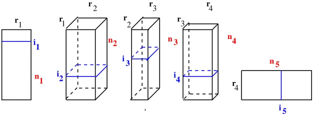
Example 1.1. Figure 1.1 illustrates the TT representation of a 5th-order tensor: each particular entry indexed by(i1, i2, ..., i5)is factorized as a product of five matrices, thus explaining the name MPS.
.
r r
r r r
r r
1 1
2 3
3 4
4 i
i i
i 1
2 4
5
n
n n n
n
1
2 3 4
5
2
r
3 i
Figure 1.1. Visualizing 5th-order TT tensor.
In case J0 = Jd 6= {1}, we arrive at the more general form of MPS, the so-called tensor chain (TC)
format. In some cases TC tensor can be represented as a sum of not more thanr∗TT-tensors (r∗= maxrℓ),
which can be converted to the TT tensor based on multilinear algebra operations like sum-and-compress. The storage cost for both TC and TT formats is bounded byO(dr2N),r= maxr
ℓ.
Clearly, one and the same tensor might have different ranks in different formats (and, hence, different number of representation parameters). Next example considers the Tucker and TT representations of a function related canonical tensor F := T(f) obtained by sampling of the function f(x) = x1+...+xd,
x∈[0,1]d, on the Cartesian grid of sizeN⊗dand specified byN-vectorsX
ℓ={ih}Ni=1, (h= 1/N,ℓ= 1, ..., d) and all-ones vector 1∈RN. The canonical rank of this tensor can be proven to be exactlyd, [89].
Example 1.2. We have rankT uck(F) = 2, with the explicit representation
F=
2
X
k=1 bkV
(1)
k1 ⊗. . .⊗V
(d)
kd , V
(ℓ) 1 = 1, V
(ℓ)
2 =Xℓ, [bk]∈
d
O
ℓ=1
as well as rankT T(F) = 2, due to exact decomposition,
F=X1 1⋊⋉
1 0
X2 1
⋊ ⋉...⋊⋉
1 0
Xd−1 1
⋊ ⋉
1
Xd
.
The rank-structured tensor formats like canonical, Tucker and MPS/TT-type decompositions induce the important concept of canonical, Tucker or matrix product operators (CO/TO/MPO) acting between two tensor-product Hilbert spaces, each of dimensiond,
A:X=
d
O
ℓ=1
X(ℓ)→Y=
d
O
ℓ=1
Y(ℓ).
For example, the R-term canonical operator (matrix) takes a form
A=
R
X
α=1
d
O
ℓ=1
A(αℓ), A(ℓ):X(ℓ)→Y(ℓ).
The actionAXon rank-RX canonical tensorX∈Xis defined asRRX-term canonical sum in Y,
AX=
R
X
α=1
RX
X
β=1
d
O
ℓ=1
A(αℓ)X
(ℓ)
β ∈Y.
The rank-rTucker matrix can be defined by the similar way.
In the case of rank-rTT format the respective matrices are defined as follows.
Definition 1.3. The rank-r TT-operator (TTO/MPO) decomposition symbolized by a set of factorized operatorsA, is defined by
A= X
α∈J
A(1)α1 ⊗ A
(2)
α1α2⊗ · · · ⊗ A
(d)
αd−1≡ A
(1)⋊⋉
A(2)⋊⋉· · ·⋊⋉A(d),
where A(ℓ) = [A(ℓ)
αℓαℓ+1] denotes the operator valued rℓ×rℓ+1 matrix, and where A
(ℓ)
αℓαℓ+1 : X
(ℓ) → Y(ℓ), (ℓ= 1, ..., d), or in the index notation
A(i1, j1, . . . , id, jd) =
r1 X
α1=1 . . .
rd−1 X
αd−1=1
A(1)
α1(i1, j1)A
(2)
α1α2(i2, j2)·. . .·
· A(αdd−−1)2αd−1(id−1, jd−1)A
(d)
αd−1(id, jd). (1.2)
Given rank-rX TT-tensorX=X(1) ⋊⋉X(2) ⋊⋉· · · ⋊⋉X(d) ∈X, the action AX=Y is defined as the TT
element Y=Y(1)⋊⋉Y(2)⋉⋊· · ·⋊⋉Y(d)∈Y,
AX=Y(1)⋊⋉Y(2)⋊⋉· · ·⋊⋉Y(d)∈Y, with Y(ℓ)= [A(αℓ1)α2X
(ℓ)
β1β2]α1β1,α2β2,
where in the brackets we use the standard matrix-vector multiplication. The TT-rank ofY is bounded by rY ≤r⊙rX, where⊙means the standard Hadamard (entry-wise) product of two vectors.
To describe the index-free operator representation of the TT matrix-vector product, we introduce the tensor operation denoted by ⋊⋉∗ that can be viewed as dual to ⋊⋉: it is defined as the tensor (Kronecker) product of the two corresponding core matrices, their blocks being multiplied by means of a regular matrix product operation. Now with the substitution Y(ℓ)=A(ℓ)⋊⋉∗X(ℓ)the matrix-vector product in TT format takes the operator form,
As an example, we consider the finite difference negatived-Laplacian over uniform tensor grid, which is known to have the Kronecker rank-drepresentation,
∆d=A⊗IN ⊗...⊗IN +IN ⊗A⊗IN...⊗IN +...+IN ⊗IN...⊗A∈RN
⊗d×N⊗d
, (1.3)
withA= ∆1= tridiag{−1,2,−1} ∈RN×N, andIN being theN×N identity matrix.
For the canonical rank we haverankCan(∆d) =d, while the TT-rank of ∆dis equal to 2 for any dimension
due to the explicit representation [50],
∆d=∆1 IN⋊⋉
IN 0
∆1 IN
⊗(d−2)
⋊ ⋉
IN
∆1
,
where the rank product operation “⋊⋉” in the matrix case is defined as above [50]. The similar statement is true concerning the Tucker rank,rankT uck(∆d) = 2.
1.2.
Quantics tensor approximation of function related vectors
In the case of large mode size, the asymptotic storage cost for a class of function relatedN-dtensors can be reduced toO(dlogN) by using quantics-TT (QTT) tensor approximation method [67,68]. The QTT-type approximation of anN-vector withN=qL,L∈N, is defined as the tensor decomposition (approximation)
in the canonical, TT or more general formats applied to a tensor obtained by theq-adic folding (reshaping) of the target vector to anL-dimensionalq×...×qdata array (tensor) that is thought as an element of the
L-dimensional quantized tensor space.
In particular, in the vector case, i.e. ford= 1, a vectorX = [X(i)]i∈I ∈WN,1,is reshaped to its quantics image inQq,L=NLj=1Kq, K∈ {R,C},byq-adic folding,
Fq,L:X →Y= [Y(j)]∈Qq,L, j={j1, ..., jL}, with jν∈ {1,2, ..., q}, ν= 1, ..., L,
where for fixedi, we haveY(j) :=X(i), andjν =jν(i) is defined viaq-coding, jν−1 =C−1+ν,such that
the coefficientsC−1+ν are found from theq-adic representation ofi−1,
i−1 =C0+C1q1+· · ·+CL−1qL−1≡
L
X
ν=1
(jν−1)qν−1.
Ford >1 the construction is similar [68].
Suppose that the quantics image for certainN-dtensor (i.e. an element ofD-dimensional quantized tensor space with D = dlogqN = dL) can be effectively represented (approximated) in the low-rank canonical
or TT format living in the higher dimensional tensor space Qq,dL. In this way we introduces the QTT
approximation of anN-dtensor. For given rank{rk}, (k= 1, ..., dL) QTT approximation of anN-dtensor
the number of representation parameters can be estimated by
dqr2logqN ≪Nd, where rk ≤r, k= 1, ..., dL,
providing log-volume scaling in the size of initial tensorO(Nd). The optimal choice of the baseqis shown to
beq= 2 orq= 3 [68], however the numerical realizations are usually implemented by using binary coding, i.e. forq= 2.
Theprincipal questionarises: either there is the rigorous theoretical substantiation of the QTT approx-imation scheme that establishes it as the new powerful approximation tool applicable to the broad class of data, or this is simply the heuristic algebraic procedure that may be efficient on certain numerical examples. The answer is positive: the power of QTT approximation method is due to the perfect rank-r decom-position discovered in [67] for the wide class of function-related tensors obtained by sampling a continuous functions over uniform (or properly refined) grid:
• r= 1 for complex exponents,
• r≤m+ 1 for polynomials of degreem,
• r is a small constant for some wavelet basis functions, etc.
all independently on the vector size N and all applicable to the general caseq= 2,3, ....
Note that the name quantics (or quantized) tensor approximation (with a shorthand QTT) originally introduced in 2009 by [67] is reminiscent of the entity “quantum of information”, that mimics the minimal possible mode size (q= 2 or q= 3) of the quantized image. Later on the QTT approximation method was also renamedvector tensorization[37].
It is worth to comment that imposing different names for the same tensor approximation method may lead to confusions in historical surveys on the topic. For example,§14 in monograph [41], actually describing the quantized tensor approximation method, designates this approach as the vector tensorization following the preprint [37] (2010), but missing the reference on the original MPI MiS preprint [67] (2009) published merely one year earlier, where the method was introduced (and analyzed theoretically) as quantics-TT (QTT) approximation for vectors. A recent survey paper [42] presents yet another misleading interpretation by suggesting that the original name of the approach is the vector tensorization introduced in preprint [37], and stating that the quantics-TT (QTT) method has appeared later in 2011 in the journal version [68]. Notice that the notion “QTT tensor approximation” has been since 2009 recognized in the literature as the common notation (see, for example [78]) for this efficient tensor approximation tool, now applied to various nontrivial multidimensional models. This remark is an attempt to establish correct chronology in the development of the QTT approximation techniques.
Concerning the matrix case, it was first found in [100] by numerical tests that in some cases the dyadic reshaping of anN×N matrix withN= 2Lmay lead to a small TT-rank of the resultant matrix rearranged
to the tensor form. The efficient low-rank QTT representation for a class of discrete multidimensional operators (matrices) was proven in [50, 80]. Moreover, based on the QTT approximation, the important algebraic matrix operations like FFT, convolution and wavelet transforms can be performed in O(log2N) complexity [23, 51, 76] (see also §1.4 below).
The recently introduced combined two-level Tucker-TT [68] and QTT-Tucker [22] formats encapsulate the benefits of the Tucker, TT and QTT representations and relax certain disadvantages of their independent use. The numerical experiments clearly indicate that the two-level QTT-Tucker format outperforms both the TT and global QTT representations applied independently due to systematic reduction of the effective tensor ranks.
To conclude this section we note that the remarkable property concerning the uniform in the grid size
N bound on the QTT-ranks for some classes of function related vectors (tensors) may address the natural question: is there some meaningful interpretation of quantized tensor formats in the infinite dimensional setting ? The constructive answer on this question should take into account the following issues: (a) the targetN-vector,N = 2L, is likely to represent a sequence of continuous functions corresponding to different
Lso that one may expect the continuous limit asL→ ∞; (b) the QTT representation of interest is supposed to be used as an intermediate quantity involved in the solution of certain PDE, so that it would be possible to calculate functionals and operators on such an element involved in the solution process designed in the quantized tensor space. The latter is exactly the point why the QTT representation of the basic partial differential operators and functional transforms (say, discrete elliptic operators, FFT, wavelet, and circulant convolution) were also in the focus of the QTT approximation theory (see also §1.4). The more detailed discussion on this intriguing topic will be addressed in the forthcoming papers.
1.3.
Functions in quantized tensor spaces
The simple isometric folding of a multi-index data array into the 2×2×...×2 format leaving in the virtual (higher) dimension D =dlogN is the conventional reshaping operation in computer data representation. The most gainful features of numerical computations in the quantized tensor space appear via the remarkable rank-approximation properties discovered for the wide class of function-related vectors/tensors [68].
Next lemma presents the basic results on the rank-1 (resp. rank-2)q-folding representation of the expo-nential (resp. trigonometric) vectors.
Lemma 1.4. ( [68]) For given N = qL, with q = 2,3, ..., L ∈ N, and z ∈ C, the exponential N-vector,
Z :={xn=zn−1}Nn=1,can be reshaped by theq-folding to the rank-1,q⊗L-tensor,
Fq,L:Z 7→Z=⊗Lp=1[1zq p−1
The number of representation parameters specifying the QTT image is reduced dramatically fromN toqL. The trigonometric N-vector, T =ℑm(Z) := {tn = sin(ω(n−1))}Nn=1, ω ∈R, can be reshaped by the successiveq-adic folding
Fq,L:T 7→T∈Qq,L,
to the q⊗L-tensorT, which has both the canonical C-rank, and the TT-rank equal exactly 2. The number of
representation parameters does not exceed4qL.
Example 1.5. In the caseq= 2, the singlesin-vector has the explicit rank-2QTT-representation in{0,1}⊗L
(see [23, 101]) withkp= 2p−Lip−1,ip∈ {0,1},
T 7→T=ℑm(Z) = [sinωk1cosωk1]⋊⋉Lp=2−1
cosωkp −sinωkp
sinωkp cosωkp
⋊ ⋉
cosωkL
sin ωkL
.
Other results on QTT representation of polynomial, Chebyshev polynomial, Gaussian-type vectors, multi-variate polynomials and their piecewise continuous versions have been derived in [68] and in subsequent papers [24, 37, 80], substantiating the capability of numerical calculus in quantized tensor spaces.
In computational practice the binary coding representation with q = 2 is the most convenient choice, though the Euler numberq∗= e≈2.7...is shown to be the optimal value [68]).
The following example demonstrates the low-rank QTT approximation can be applied for O(|logε|) complexity integration of functions. Given continuous function f(x) and weight function w(x), x∈[0, A], consider the rectangular N-point quadrature, N = 2L, ensuring the error bound |I−IN| = O(2−αL).
Assume that the corresponding functional vectors allow low-rank QTT approximation. Then the rectangular quadrature can be implemented as the scalar product on QTT tensors, inO(logN) operations.
Z 1
−1
w(x)f(x)dx≈IN(f) :=h N
X
i=1
w(xi)f(xi) =hW,FiQT T, W,F∈ L
O
ℓ=1
R2.
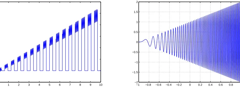
Example 1.6 illustrates the uniform bound on the QTT rank for nontrivial highly oscillating functions and with choicew(x) = 1, see Figure 1.3. Here and in the following the threshold error likeǫQT T corresponds to
the Euclidean norm.
0 1 2 3 4 5 6 7 8 9 10 −2
0 2 4 6 8 10 12
−1 −0.8 −0.6 −0.4 −0.2 0 0.2 0.4 0.6 0.8 1 −2
−1.5 −1 −0.5 0 0.5 1 1.5 2
Figure 1.2. Visualizing functions f3 (left) andf4.
Example 1.6. Highly oscillated and singular functions on [0, A],ω= 100,ǫQT T = 10−6,
f3(x) =
x+aksin(ωx), x∈10
k−1
p ;
k−0.5
p
i
0, x∈10k−0.5
p ;
k p
i
where functionf3(x),x∈[0,10],k= 1, ..., p,p= 16,ak = 0.3 + 0.05(k−1), is recognized on three different
scales.
The average QTT rank over all mode ranks for the corresponding functional vectors are given in the next table. The maximum rank over all the fibers is nearly the same as the average one.
N\r rQT T(f3) rQT T(f4)
214 3.5 6.5 215 3.6 7.0 216 3.6 7.5 217 3.6 7.9
Table 1.1. Average QTT ranks ofN-vectors generated byf3 andf4.
Notice that 1D and 2D numerical quadratures based on interpolation by Chebyshev polynomials have been developed [40]. Taking into account that Chebyshev polynomial sampled on Chebyshev grid has exact rank-2 QTT representation [68], allows us the efficient numerical integration by Chebyshev interpolation using the QTT approximation.
1.4.
Operators in quantized tensor spaces
This section discusses the quantised representation of operators/matrices. The explicit low-rank QTT representations for the wide class of discrete elliptic operators (FEM/FDM matrices) was recently developed in [25, 50, 51, 68, 80].
As the first result is this direction the explicit rank-3 QTT representation of ∆1 was introduced [50],
∆1 = I J′ J⋊⋉ I J
′ J
J J′
⊗(d−2)
⋊ ⋉
2I−J−J ′
−J
−J′ ,
with the Pauli matrices
I=
1 0 0 1
, J =
0 1 0 0
.
Other results concerning QTT representation of ∆dand its inverse ford≥2 are collected in Proposition 1.9
below.
The analysis of the low QTT-rank approximations of elliptic operator inverse ford≥2 is based on certain assumptions on the QTT-rank of the matrix exponential family.
Conjecture 1.7. For any given ε > 0, and for fixed a, b > 0, the family of matrix exponentials,
{exp(−tk∆1)}, tk > 0, k = −M, ..., M, allows the QTT ε-approximation with rank-r∆ being uniformly bounded in the grid size N and in the scaling factors tk ∈ [a, b] ⊂ R>0 (see Table 1.2 for numerical justification).
Table 1.2 represents the average QTT-ranks in approximation of certain function related matrices up to fixed toleranceεQT T = 10−5. It includes the important example of matrix exponential (cf. Conjecture 1.7).
The matrixA=diag(f(kxk2)), (x= (x
1, x2),|xi| ≤1) is a diagonal matrix with diagonal entries obtained
by sampling a functionf(kxk2) over uniform grid points situated on the diagonalx 1=x2.
We observe that rank parameters depend very mildly on the grid size. We note that the QTT ranks
N\r e−α∆1, α= 0.1/1/10/102 diag(1/kxk2) diag(e−kxk2)
29 6.2/6.8/9.7/11.2 5.1 4.0 210 6.3/6.8/9.5/10.8 5.3 4.0 211 6.4/6.8/9.0/10.4 5.5 4.1
of the matrix A = diag(f(kxk2)) coincides with those for the generating vector X that follows from the explicit QTT representations (see Def. 1.3). Given vector X and the corresponding rank-rX QTT-tensor
X=X(1)⋊⋉X(2)⋊⋉· · ·⋊⋉X(d)∈X, then the QTT representation of the matrixA=diag(X) is given by
A=A(1) ⋊⋉A(2) ⋊⋉· · ·⋊⋉A(d), A(2)=diag(X(k)),
wherediag(X(k)) is the matrix diagonalization of the core tensorX(k). Define the anisotropicd-Laplacian
∆d,α:= d
X
ℓ=1
αℓ d
O
k=1 ∆δℓ−k
1 , αℓ>0, δm is the Kronecker symbol. (1.5)
Now we can prove the following Lemma (see [68]).
Lemma 1.8. Under claims of Conjecture 1.7 on the QTT-rank of the univariate matrix exponentials, there exist C, β >0independent of d, such that for allM ∈N,
k∆−d,α1 −BMk ≤Ce−β
√
M, β >0, (1.6)
whereBM is defined as
BM := M
X
k=−M
ck d
O
ℓ=1
exp(−tkαℓ∆1), tk=ekh, ck =htk, h=π/
√
M . (1.7)
Lemma 1.8 implies that the matrix family{BM}possesses the low-rank approximation (or preconditioner
ifM is small) to the anisotropic d-Laplacian inverse ∆−1d,α, whose ranks scale likeO(log2ε), whereεis the error threshold. The constant β >0 depends logarithmically on the grid sizeN, whileC scales linearly in the norm of inverse matrixk∆−d,α1k.
The following statement summarizes the previous discussion and the related results in [50].
Proposition 1.9. Ford≥2 the canonical, TT and QTT rank estimates hold:
rankC(∆d) =d, rankT T(∆d) = 2, rankQT T(∆d) = 4.
rankQT T(∆1) = 3, rankQT T(∆−11)≤5.
Given ε >0, then for theε-rank we have
rankT T(∆−d1)≤rankC(∆d−1)≤C|logε|logN. (1.8)
Moreover, under claims of Conjecture 1.7 there holds
rankQT T(∆−d1)≤C|logε|
2logN. (1.9)
In both cases the constant C does not depend ond.
Thed-dimensional FFT overN⊗d grid can be realized on the rank-k tensor with the linear-logarithmic
costO(dkNlog2N), due to the rank-1 factorized representation
FN(d)= (F
(1)
N ⊗I...⊗I)(I⊗F
(2)
N ...⊗I)...(I⊗I...⊗F
(d)
N )≡F
(1)
N ⊗...⊗F
(d)
N ,
whereFN(ℓ)∈RN×N represents the univariate FFT matrix along mode ℓ.
The super-fast Fourier transform ofN-dtensors can be computed in log-volume complexity, O(dlog2N), by using the QTT approximation as proposed in [23].
The super-fast convolution transform of the complexityO(dlog2N) using the explicit QTT representation of multilevel Toeplitz matrices is developed in [51].
The super-fast QTT wavelet transform of logarithmic complexity by the exact low-rank representation of the wavelet transform matrix was described in [76] (see also [105] for the related discussion).
1.5.
Multilinear algebra and tensor-rank truncation
Low-parametric tensor formats provide prerequisites for multidimensional algebraic calculus since the stor-age complexity of rank-structured tensors scales linearly in dimension d. However, the numerical capability ofε-truncated tensor operations is essentially determined by the following issues:
• Understanding of nonlinear tensor approximation in the canonical, Tucker, and MPS/TT formats
• Developments on efficient multilinear algebra and rank optimization algorithms
• Approximation theory for functions and operators in (quantized) tensor spaces
• Construction of stable iterative methods for solving multidimensional PDEs in tensor formats. It is worth to note that the important multilinear algebraic operations with canonical, Tucker and TT tensors can be implemented with linear complexity scaling in the univariate mode sizeNand in the dimension
dby representing them in terms of tensor operations on rank-1 elements.
For example, following [72], for the rank-R1 and rank-R2 canonical tensorsX,Y∈RI,I :={1, ..., N}d, we have
hX,Yi=
R1 X
k=1
R2 X
m=1
d
Y
ℓ=1 D
X(kℓ),Y
(ℓ)
m
E ,
while the Hadamard product is computed by
X⊙Y:=
R1 X
k=1
R2 X
m=1
X(1)k ⊙Y
(1)
m
⊗. . .⊗X(kd)⊙Y
(d)
m
.
We define thediscrete convolution productof two convolving tensors [72] by
X∗Y:= "
X
k∈I
XkYj−k
#
j∈J
, J :={1, ...,2N−1}d.
The convolution product of two tensors in the canonical format can be realized inO(dR1R2NlogN) opera-tions [72] relying on the representation
X∗Y:=
R1 X
k=1
R2 X
m=1
X(1)k ∗Y
(1)
m
⊗. . .⊗X(kd)∗Y
(d)
m
∈RJ, (1.10)
where X(kℓ)∗Y
(ℓ)
m ∈R2N−1denotes the convolution product ofN-vectors defined as
X(kℓ)∗Y
(ℓ)
m =
" n X
n=1
xnyj−n
#
j
, j= 1, ...,2N−1.
Hence, the one-dimensional convolution can be performed by FFT inO(NlogN) operations. Similarly, the above mentioned tensor operations for Tucker tensors can be reduced to 1D linear algebra [69, 72].
The formatted implementation of the scalar product of TT tensors [99]
hX,Yi=hX⊙Y,1i
can be performed by using the Hadamard product in TT formatZ=X⊙Y: Z(k)
ik =X
(k)
ik ⊗Y
(k)
ik .
in O(dlogN) operations and storage costs. This allows fast computations on large spatial grids without practical limitations onN, whereN is usually associated with the univariate grid size.
Representation of tensors in low separation rank formats is the key point in the design of fast tensor-structured numerical methods for large-scale higher dimensional simulations. In fact, it allows the implemen-tation of basic linear and bilinear algebraic operations on tensors mentioned above with linear complexity in the univariate tensor size (see [23, 50, 55, 69, 70]). However, the bilinear tensor operations normally increase the separation rank of the resultant tensor.
To perform computation over nonlinear set (manifold) of rank-structured tensorsS (say, the canonical, Tucker, MPS/TT, QTT, and QTT-Tucker formats) with controllable complexity, we need to perform a “pro-jection” of the current iterand inS0⊃ S onto that manifoldS by using the “formatted“ tensor operations. This action is fulfilled by implementing the tensor truncation operatorTS :Wn,d→ S defined by
A0∈ S0⊂Wn,d: TSA0= argminT∈SkA0−Tk, (1.11)
that reduces to a challenging nonlinear approximation problem. The replacement ofA0by its approximation inS is called thetensor truncationtoSand denoted byTSA0. In practice, the computation of the minimizer
TSA0can be performed only approximately. The setS of rank-structured tensors can be chosen adaptively in order to control the approximation errorε >0,
kA0−TSA0k ≤ε.
In the case of Tucker, TT/QTT and QTT-Tucker formats the quasi-optimal approximation can be com-puted by conventional QR/SVD algorithm [22, 36, 84, 103], also known in the physical literature as the Schmidt decomposition. In particular, the Tucker tensors can be approximated by the so-called higher order SVD (HOSVD), [21]. Robust SVD-based algorithms are applicable since the Tucker and TT ranks can be controlled by a certain matrix rank. Indeed, for MPS/TT format we have the equivalent definition in terms of the TT-unfolding matrix, T T[r] := {A ∈ Vn : rankA[p] ≤ rp, p=1,...,d-1 }, where the TT-unfolding
matrixA[p] is defined by
A[p]:=A(j1j2 . . . jp
| {z }
column ind.
;jp+1. . . jd
| {z }
row ind. ).
For the Tucker format we have the alternative definition T[r] := {A ∈ Vn : rankA(p) ≤ rp, p = 1, ..., d},
where the Tucker unfolding matrixA(p)is defined by
A(p):=A(j1j2 . . . jp−1
| {z }
row ind.
; jp
|{z} column ind.
;jp+1. . . jd
| {z }
row ind. ).
In turn, the canonical and TC ranks can not be identified with certain matrix ranks that may result in instabilities of approximation schemes. Approximation in theR-term canonical format is considered as a subtle problem that cannot in general be solved by a stable algorithms in polynomial cost. One of the reasons is that the set of canonical tensors with rank≤Ris not closed as shown by the following example.
Example 1.10. The tensorF, withrankCan(F) =d, generated by sampling of the functionf(x) =x1+...+xd on a tensor grid can be approximated with arbitrary precision by rank-2 elements
F= lim
ε→0 Nd
ℓ=1(1 +εXℓ)−1
ε .
However, for some classes of functions and operators the robust analytic methods based onR-term explicit sinc-quadrature approximations can be successfully applied (see [70] and references therein).
2.
Tensor numerical methods for
d
-dimensional PDEs
In this section, we discuss the benefits of tensor numerical methods (TNM) in two important applica-tions: the nonlinear Hartree-Fock (HF) equation in electronic structure calculations (§2.1) and the real-time parabolic equations in many-particle dynamics (§2.2).
The numerical challenge in the HF calculations is due to the presence of large number of complicated convolution-type integrals in R3, multiply recomputed within the iterations on nonlinearity, as well as hard complexity scaling of the traditional methods with respect to the size of a molecular system (see for example [90, 109] and references therein). At this point the beneficial features of tensor computations has been successfully realized in the form of fast grid-based black-box HF-solver that manifests linear complexity in the univariate grid size [55,56,60,73,74]. The latter can be reduced to the logarithmic scale by implementation in quantized tensor spaces [59]. Further steps toward TNMs for post Hartree-Fock calculations [58], and for solving the Hartree-Fock problem for large lattice-structured and periodic systems [61, 62] are the subject of current research.
The real space numerical methods combined with FEM approximations have become attractive in elec-tronic structure calculations as the possible alternative to the traditional approaches (see [15,33,46,75,88,108] and references therein).
For a class of multi-dimensional parabolic problems including, in particular, the molecular Schr¨odinger, the Fokker-Planck and master equations, the computational challenges arise due to the curse of dimensionality. We discuss the main issues which allow to understand how the d-dimensional dynamics can be simulated in quantized tensor spaces with the linear complexity in d and in log-log complexity in the mesh size for simultaneous space-time discretization. Further details can found in [24, 25, 35, 70]. Exposition of tensor methods based on the Dirack-Frenkel variational principle implemented on the Tucker and MPS/TT tensor manifolds can be found in [92, 93, 102] and references therein.
Recently, the TNM were shown to be efficient for solving parameter dependent PDEs in the case of high dimensional parametric space [12, 26, 77, 82].
Another popular topic in numerical analysis of multidimensional PDEs is concerned with the so-called greedy methods and their applications [9, 18, 32, 91], which became attractive since the simplicity of greedy algorithms: the main step usually includes either rank-1 corrections low-rank tensors in other formats com-monly used in practice. Due to the page limits, these topics will not be further addressed in this paper.
2.1.
Hartree-Fock equation in electronic structure calculations
2.1.1. Problem settingThe HF equation for determination of the ground state energy of a molecular system consisting ofM nuclei andNorb electrons (closed shell case) is given by the following nonlinear eigenvalue problem inH1(R3) [90],
(Fφi)(x) =λiφi(x),
Z
R3
φi(x)φj(x) dx=δij, i, j= 1, ..., Norb, (2.1)
where the non-linear integral-differential Fock operatorF is given by
F:=−12∆−Vc+VH+VE, Vc = M
X
ν=1
Zν
kx−Aνk
, (2.2)
with the Hartree potential, VH(x), and the nonlocal exchange operator, VE, defined by
VH(x) :=
Z
R3
τ(y, y)
kx−ykdy, and VEφ:=−
1 2
Z
R3
τ(x, y)
kx−ykφ(y) dy,
respectively. Here, 1/k · k : R3 → R corresponds to the Newton potential, andZν ∈ R+, Aν ∈ R3 (ν =
1, ..., M) specify charges and positions ofM nuclei. The electron density matrixτ :R3×R3 →R, is given byτ(x, y) = 2PNorb
i=1 φi(x)φ∗i(y),specifying the electron densityρ(x) =τ(x, x).
This dependence is expressed by the 3D convolution transform with the Newton convolving kernel, while the electron densityρ(x) contains multiple strong singularities corresponding to each nuclei location. There-fore solution of the HF equation requires iterative solvers, with multiply repeated recalculation of these convolution integrals.
Usually, the Hartree-Fock equation is approximated by the standard Galerkin projection of the initial problem (2.1) posed inH1(R3) (see [90] for more details). For a given finite Galerkin basis set{g
µ}1≤µ≤Nb, gµ∈H1(R3), the molecular orbitalsφi are expanded (approximately) by
φi = Nb X
µ=1
Cµigµ, i= 1, ..., Norb, (2.3)
yielding the Galerkin system of nonlinear equations for the coefficients matrix C = {cµi} ∈ RNb×Norb,
concatenating the eigenvectorsCi ∈RNb (and the density matrixD= 2CC∗∈RNb×Nb)
F(D)C=SCΛ, Λ =diag(λ1, ..., λNb), C
TSC=I
Nb, (2.4)
whereS is the overlap (stiffness) matrix for{gµ}1≤µ≤Nb, and the Fock matrix
F(D) =H+J(D) +K(D), (2.5)
is a sum of the stiffness matrix H = {hµν} of the core Hamiltonian H = −12∆ +Vc (the single-electron
integrals),
hµν =
1 2
Z
R3∇
gµ· ∇gνdx+
Z
R3
Vc(x)gµgνdx, 1≤µ, ν≤Nb,
and the two nonlinear terms J(D) +K(D), representing the Galerkin approximation to the Hartree and exchange operators. This is the main computational task, which is traditionally calculated by using the two-electron integrals tensorB= [bµνκλ], defined as follows: Given the finite basis set{gµ}1≤µ≤N
b,gµ∈H 1(R3),
the associated fourth order two-electron integrals (TEI) tensor,B= [bµνκλ], is defined entrywise by
bµνκλ=
Z
R3 Z
R3
gµ(x)gν(x)gκ(y)gλ(y)
kx−yk dxdy, µ, ν, κ, λ∈ {1, ..., Nb}. (2.6)
In the straightforward implementation based on the analytically precomputed integrals, the computational and storage complexity for the TEI tensor is of order O(N4
b), or evenO(Nb5), that becomes non-tractable
already forNb of order of several hundred.
Given TEI tensor, theNb×Nb matricesJ(D) andK(D) can be represented by
J(D)µν = Nb X
κ,λ=1
bµν,κλDκλ, K(D)µν =−1
2
Nb X
κ,λ=1
bµλ,νκDκλ, (2.7)
with the low-rank symmetric density matrix, D = 2CCT ∈ RNb×Nb, such that rank(D) = N
orb ≪ Nb.
Equations (2.7) can be rewritten in terms of the TEI matrix B= [bµν,κλ]∈RN
2 b×N
2 b. The total energy is computed as
EHF = 2 NXorb
i=1
λi− NXorb
i=1
e Ji−Kei
,
where Jei = (φi, VHφi)L2 = hCi, JCii and Kei = (φi, Kφi)L2 =hCi, KCii, i= 1, ..., Norb, are the Coulomb
and exchange integrals in the basis of orbitalsφi. The resulting ground state energy of a molecule,E0, for
the given geometry of nuclei, includes the nuclei repulsion energyEnuc,
E0=EHF +Enuc, where Enuc= M
X
k=1
M
X
m<k
ZkZm
kxk−xmk
The standard quantum chemical implementations are based on the analytically precomputed set of the two-electron integrals (2.6) in a naturally separable Gaussian basis with the computational and storage complexity for the TEI tensor of order O(N4
b), or even O(Nb5), that becomes non-tractable already for Nb
of order of several hundred.
2.1.2. Grid-based tensor numerical methods
The tensor-structured numerical methods, both the name and the concept, appeared during the work on the 3D grid-based tensor approach to the solution of the Hartree-Fock equation. They lead to “black-box” numerical treatment of the Hartree-Fock problem based on the low-rank representation of the basis functions in a volume box, using then×n×n3DCartesian grid positioned arbitrarily with respect to the atomic centers [55,57,60,74]. In 2008 [54,73] it was shown that within the tensor-structured paradigm the core Hamiltonian and the 3D convolutions with the Newton kernel, involved in the Coulomb and exchange operators, can calculated in 1Dcomplexity by the rank-structured tensor operations reduced to 1Dconvolutions, Hadamard and scalar products [56, 69, 73]. Due to elimination of the analytical integrability requirements it gives a choice to use rather general physically relevant basis sets represented on the grid. High accuracy is achieved due to grid-sizes up to the order ofn≃106, yielding a volume box of sizen3≃1018. It corresponds to mesh resolution up to h= 10−5 A◦ (close to sizes of atomic radii) in the volume box with the equal sizes of 20 A◦ for each spatial variable. Matlab on a Sun station is used for all algorithms, without parallelizations and supercomputing.
Chronologically, two different approaches have been developed for the 3D grid-based tensor-structured solution of the HF equation. Both use the rank-structured calculation of the core Hamiltonian [56, 57] for a given grid-based basis set.
• The tensor solver I does not use the two-electron integrals. Instead, the Coulomb and exchange operators are recomputed “on the fly” using the refined 3D grids and rank-structured (1D) opera-tions. [54, 55, 74]. This approach has low storage demand, but might be time consuming. It can be applicable to the Kohn-Sham type models.
• The “black-box“ solver II based on calculation of the TEI matrix B by the truncated Cholesky decomposition and the redundancy-free factorization by the algebraically reduced product basis yielding the reduced storage consumptionO(N3
b) [56, 58, 59]. Its performance in time and accuracy
is compatible with the benchmark packages in quantum chemistry based on analytical pre-calculation of involved multidimensional integrals.
In the following, we briefly discuss the tensor algorithm for computation of TEIs used in the solver II. We suppose that all basis functions{gµ}1≤µ≤Nb, are supported by the finite volume box Ω = [−b, b]
3∈R3, and assume, for ease of presentation, thatrank(gµ) = 1. Introducing then×n×nCartesian grid over Ω and
using the standard collocation discretization in the volume by piecewise constant basis functions, we define a grid-based tensor representation of the initial basis set gµ(x)∈R3,µ= 1, . . . Nb,
gµ(x) =gµ(1)(x1)g(2)µ (x2)gµ(3)(x3)≈Gµ=G(1)µ ⊗G(2)µ ⊗G(3)µ ∈Rn×n×n.
Define the respective product-basis tensor
G= [Gµν]∈RNb×Nb×n
⊗3
with Gµν=Gµ⊙Gν∈Rn
⊗3 ,
where µ, ν∈ {1, ..., Nb}, then both the TEI tensor and matrix are represented by tensor operations,
B=G×n⊗3P∗n⊗3G, bµν,κλ=hGµν,P∗Gκλi
n⊗3. (2.9)
Here the rank-RN canonical tensorP =
RPN
k=1
Pk(1)⊗Pk(2)⊗Pk(3) ∈Rn⊗3 approximates the Newton potential
1
kxk (see [13, 73] for more details), ∗ stands for the 3D tensor convolution, and ⊙ denotes the Hadamard product of tensors.
Though tensor methods reduce the multidimensional integration to 1D complexity operations, the direct tensor-structured evaluation of (2.9) needs a storage size of at least, O(RNNb2n), which can be prohibitive
approximating its site matrices,G(ℓ)∈Rn×N2
b, (ℓ= 1,2,3) in a “squeezed” factorized form,G(ℓ)∼=U(ℓ)V(ℓ)T, according to the chosenε-truncation. This step can be implemented by the truncated SVD in combination with incomplete truncated Cholesky decomposition.
This provides the construction of dominating subspaces in thex-, y- andz- components in the product basis set defined by an n×Rℓ matrix U(ℓ) (left orthogonal basis) andNb2×Rℓ matrixV(ℓ) (right basis).
Then for the TEI matrixB∈RNb2×N 2
b, we obtain a factorization [58, 60],
B∼=Bε:=
RN
X
k=1
⊙3ℓ=1V(ℓ)M (ℓ)
k V
(ℓ)T, (2.10)
whereV(ℓ)is the corresponding right redundancy-free basis,⊙denotes the point-wise (Hadamard) product of matrices, and
Mk(ℓ)=U(ℓ)T(Pk(ℓ)∗nU(ℓ))∈RRℓ×Rℓ, k= 1, ..., RN. (2.11) Ultimately, the TEI matrixB is approximated in a form of the truncated Cholesky factorization,B≈LLT,
L∈RNb2×RB (R
B=O(Nb)), such that the required columns ofB are easily computed by using (2.10).
Vectorizing matrices J = vec(J(D)), K = vec(K(D)), D = vec(D), we arrive at the simple matrix representations,
J =BD≈L(LTD), vec(K) =K=BD,e (2.12)
whereBe=mat(Be) is the matrix unfolding of the permuted tensor Be = [ebµνκλ] such thatebµνκλ=bµκνλ. The nonlinear eigenvalue problem (2.4) is solved by the commonly used DIIS self-consistent iteration which requires the update of both Hartree and exchange operators at each iterative step.
2.1.3. Numerical illustrations
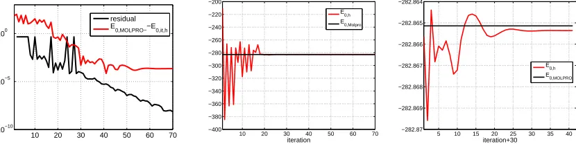
Figure 2.1, left, illustrates the convergence history for self-consistent iterations by tensor solver II compared with the output of a standard quantum chemical package MOLPRO based on analytical calculations [123] for the Glycine amino acid,C2H5N O2. The basis set cc-pVDZ of 170 Gaussians is used for both analytical and 3D grid-based calculations. Here TEI is calculated on the grids n3 = 1310723. For this iteration the core Hamiltonian is taken from MOLPRO. Time for one iteration is about 6 seconds in Matlab.
10 20 30 40 50 60 70 10−10
10−5 100
residual E
0,MOLPRO−−E0,it,h
10 20 30 40 50 60 70 −400
−380 −360 −340 −320 −300 −280 −260 −240 −220 −200
iteration E
0,h E0,Molpro
5 10 15 20 25 30 35 40 −282.87
−282.869 −282.868 −282.867 −282.866 −282.865 −282.864
iteration+30 E0,h E
0,MOLPRO
Figure 2.1. Left: iterations history for Glycine molecule with TEI calculated on the grids n3= 1310723. Middle: convergence in energy. Right: a zoom for energy difference at last iteration.
We observe, that though the residual displays good convergence (in max-norm), the error with respect to analytical calculations stagnates at 2·10−4 (relative error < 7·10−7). Figure 2.1 middle, shows the convergence in ground state energy E0,it,h while the right figure displays the zoomed difference of ground
state energy for last iterations. Here the energy E0,it,h is computed by (2.8) at each iteration step it
representing the convergence history. The stagnation in the energy on lower than MOLPRO level (relative error 7·10−7) may indicate the actual accuracy in computation of 3D convolution integrals in that code, and, beside, some possible instabilities of the grid-based algorithms applied for huge spatial grids (n3= 1310723). This topic needs further analysis to be done elsewhere.
Figure 2.2. Left: the error in density matrix resulting from calculations of TEI on a grid of sizen3= 655363. Middle: the same error for the grid sizen3= 1310723. Right: the error in density matrix for Alanine amino acid, TEI computed with n3= 327683.
n3 = 1310723 (middle). Figure 2.2 (right) shows the error of tensor calculations for Alanine amino acid,
C3H7N O2, with TEI computed on the gridn3= 327683, withNb2= 2112 basis functions.
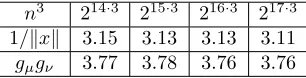
The dominating part in the above tensor calculus resulted by rather large mode size n, can be reduced to the logarithmic scale in lognby applying the QTT approximation. Numerical illustrations on the QTT approximation of functions and operators arising in the solution of Hartree-Fock equation are given in Table 2.1. It indicates the low QTT-rank approximability of (a) the canonical vectors in low-rank decomposition
n3 214·3 215·3 216·3 217·3 1/kxk 3.15 3.13 3.13 3.11
gµgν 3.77 3.78 3.76 3.76
Table 2.1. Average QTT-ranks for canonical vectors of the tensorP, and for the product basis{gµgν} designed for CH4 molecule.
P of the Newton kernel 1/kxk, in R3, see [73], (b) the product basis set designed for CH4 molecule, both discretized over large n×n×n spatial grids. In all cases the QTT approximation accuracy ε = 10−6 is achieved. We observe that QTT-ranks of canonical vectors for both the Newton potential and the product basis remain practically constant inn, ensuringO(logε−1logn) complexity scaling.
These results show that the grid-based tensor-structured Hartree-Fock solver II provides the accuracy and computation time compatible with the analytical calculations from MOLPRO. More numerical results, including the complete grid-based calculations with the grid-based core Hamiltonian and their comparison with MOLPRO are given in [56]. The Laplacian in core Hamiltonian is calculated on large 3D grids by using the QTT format.
We summarize that tensor numerical methods described above are implemented in the Matlab program package Tensor-based Electronic Structure Calculation (TESC) by V. Khoromskaia and B. Khoromskij. TESC package allows the efficient grid-based solution of the 3D nonlinear Hartree-Fock equation discretized in a general set of basis functions characterized by the existence of low-rank separable representation. All 3D and 6D integrals involved are approximated on large n×n×ngrids and computed by the black-box algorithms in the 1D complexity, O(n), or even inO(logn) operations, which allows us the high resolution with the grid size up ton= 106.
Further work should be focused, in particular, on the developments of the general type basis functions. Now preliminary results are obtained for products of Gaussians with the plane waves.
2.1.4. Tensor method for fast lattice summation
The recent progress in tensor numerical methods for Hartree-Fock calculations is concerned with the generalization of the above mentioned approach to the case of large lattice structured and periodic systems [61, 62] arising in the modeling of cristalline, metallic and polymer type compounds.
To fix the idea, we consider the electrostatic potentialVc(x) in (2.2) in the simplest caseM = 1. Defined
symmetric box
ΩL=B×B×B, with B = b
2[−L, L], L∈N,
consisting of a union of L×L×Lunit cells Ωk, obtained from Ω0 by a shift specified by the lattice vector bk, where k = (k1, k2, k3)∈Z3, −(L−1)/2≤kℓ ≤(L−1)/2, (ℓ = 1,2,3). Here L= 1 corresponds to a
system in the unit cell. Recall that b =nh, where h > 0 is the mesh size that is the same for all spatial variables, and n is the number of grid points for each variable. We also define the accompanying domain e
ΩL obtained by scaling of ΩL with the factor of 2, ΩeL= 2ΩL, and introduce the respective rank-Rmaster
tensorPe =
R
P
q=1 e
Pq(1)⊗Peq(2)⊗Peq(3), approximating k1xk in ΩeL on tensor grid with mesh sizeh.
In the case of extended system in a box the summation problem for the total potentialVcL is formulated in the domain ΩL=S(kL1,k−1)2,k/32=−(L−1)/2Ωk as well as in the accompanying domain. On each Ωk⊂ΩL, the
target potentialvk(x) = (VcL)|Ωk, is obtained by summation over all unit cells in ΩL,
vk(x) =
(L−1)/2 X
k1,k2,k3=−(L−1)/2 Z0
kx−bkk, x∈Ωk. This calculation is performed at each ofL3elementary cells Ω
k⊂ΩLsimultaneously, which is implemented
by the assembled tensor summation method described in [61]. The resultant lattice sum is presented by the canonical rank-R tensorPcL∈R
nL×nL×nL,
PcL =Z0
R
X
q=1 (
(L−1)/2 X
k1=−(L−1)/2
Wk1Pe
(1)
q )⊗(
(L−1)/2 X
k2=−(L−1)/2
Wk2Pe
(2)
q )⊗(
(L−1)/2 X
k3=−(L−1)/2
Wk3Pe
(3)
q ), (2.13)
whereWkℓ is the shift-and-windowing transform along the k-grid. The numerical cost and storage size are bounded by O(RLNL), and O(RNL), respectively (see [61], Theorem 3.1), whereNL = nL, and n is the
grid size in the unit cell.
The lattice sum in (2.13) converges only conditionally asL→ ∞. This aspect was addressed in [61].
−10 −5 0 5 10 0
0.005 0.01 0.015 0.02 0.025 0.03 0.035
−6 −4 −2 0 2 4 6 0
0.005 0.01 0.015 0.02 0.025 0.03
−8 −6 −4 −2 0 2 4 6 8 0
0.005 0.01 0.015 0.02 0.025 0.03
Figure 2.3. Canonical vectors in the assembled 10×4×6 lattice sum.
Figure 2.3 demonstrates the canonical vectors for assembled tensor sum corresponding to 10×4×6 lattice.
2.2.
Real-time dynamics by parabolic equations
2.2.1. General introductionLet W be a complex Hilbert space and H be a self-adjoint positive definite operator with the domain
D(H) and the spectrum Σ(H)∈[λ0,∞), λ0 >0. Given σ∈ {−1, i}, we consider the following initial value problem
∂ψ
∂t =σHψ(t), ψ(0) =ψ0∈D(H)⊂W. (2.14)
The solution of (2.14) is represented by using operator exponential, ψ(t) = eσHtψ
0, however, in general, the solution operator of this parabolic problem, S(t) =eσHt, does not allow the accurate low-rank tensor