B. Bouchard, J.-F. Chassagneux, F. Delarue, E. Gobet and J. Lelong, Editors
NUMERICAL SCHEMES FOR THE AGGREGATION EQUATION WITH
POINTY POTENTIALS
∗Benoˆıt Fabr`
eges
1, H´
el`
ene Hivert
2, Kevin Le Balc’h
3, Sofiane Martel
4,
Franc
¸ois Delarue
5, Fr´
ed´
eric Lagouti`
ere
1and Nicolas Vauchelet
6Abstract. The aggregation equation is a nonlocal and nonlinear conservation law commonly used to describe the collective motion of individuals interacting together. When interacting potentials are pointy, it is now well established that solutions may blow up in finite time but global in time weak measure valued solutions exist. In this paper we focus on the convergence of particle schemes and finite volume schemes towards these weak measure valued solutions of the aggregation equation.
R´esum´e. L’´equation dite d’agr´egation est une loi de conservation nonlocale et nonlin´eaire fr´equemment utilis´ee pour d´ecrire le comportement collectif d’individus en interacton. Quand le potentiel d’interaction est singulier, il est dor´enavant bien connu que les solutions de l’´equation d’agr´egation explosent en temps fini. Cependant l’existence de solutions globales en temps `a valeurs mesures a ´et´e ´etablie. Dans ce travail, nous ´etudions la convergence de sch´emas particulaires et de sch´emas de volumes finis vers les solutions faibles de l’´equation d’agr´egation.
Introduction
This work is devoted to the numerical approximation of measure valued solutions to the so-called aggregation
equation inRd. This is a nonlinear and nonlocal conservation law that is commonly used to model the dynamics
of (a density of) individuals interacting together through an interaction potential. Denoting byW the interaction
potential, its gradient∇xW(x−y) measures the relative force exerted by a unit mass located at a pointyonto
a unit mass located at a pointx, and the aggregation equation reads
∂tρ= div (∇xW∗ρ)ρ
, t >0, x∈Rd. (1)
We complement this system with the initial condition ρ(0,·) =ρini.
∗The authors acknowledge support from the “BQR Accueil EC 2017” grant from Universit´e Lyon 1.
1 Univ Lyon, Universit´e Claude Bernard Lyon 1, CNRS UMR 5208, Institut Camille Jordan, 43 blvd. du 11 novembre 1918,
F-69622 Villeurbanne cedex, France.
2 Ecole Centrale de Lyon, 36 avenue Guy de Collongue, 69134 Ecully, France.
3 Univ Rennes, CNRS, IRMAR - UMR 6625, F-35000 Rennes, France.
4 Laboratoire d’hydraulique Saint-Venant ( ´Ecole des Ponts ParisTech – EDF R&D – CEREMA), Universit´e Paris-Est, 6 quai
Watier, 78401 Chatou Cedex, France.
5 Laboratoire J.-A. Dieudonn´e, UMR CNRS 7351, Univ. Nice, Parc Valrose, 06108 Nice Cedex 02, France.
6 Universit´e Paris 13, Sorbonne Paris Cit´e, CNRS UMR 7539, Laboratoire Analyse G´eom´etrie et Applications, 93430
Villeta-neuse, France.
c
EDP Sciences, SMAI 2019
This is an Open Access article distributed under the terms of the Creative Commons Attribution License (http://creativecommons.org/licenses/by/4.0), which permits unrestricted use, distribution, and reproduction in any medium, provided the original work is properly cited.
The aggregation equation is the subject of several studies since it has many applications in physics and in biology (see e.g. [23] and references therein). For instance, it may be used to describe crowd motion [15, 37], biological swarming [30, 36], granular media dynamics [14, 35], evolution of vortex densities in superconductors [3, 22, 31], aggregative phenomena in bacterial chemotaxis [21, 26], animal aggregation [12].
When considering fully attractive potentials, ∇W may have some discontinuities. This is the case, for
instance, for potentials of the typeW(x) =w(|x|) whose gradient may have a singularity in 0 even for smooth
w. It is known that in this situation, Lp weak solutions may blow up in finite time, in the sense that the Lp
norm, forp >1, blows up in finite time (see e.g. [4–6]). Since the aggregation equation is conservative, a notion
of solutions in the sense of measures has been developped, for which global-in-time existence may be obtained. Two different approaches may be found in the literature. On one side, weak measure valued solutions have been defined in [11] thanks to the theory of gradient flows for a Wasserstein metric [2]. On the other side, based on the theory of Filippov [24], weak measure valued solutions have been defined as a pushforward by a flow in [13] (see also [27] for the one dimensional case). In this latter approach, the aggregation equation is seen as a
transport equation with a velocity field∇xW∗ρwhich satisfies a one-sided Lipschitz-continuity condition (see
(5) below for the definition of one-sided Lipschitz-continuity condition). It has been also proved in [13] that both approaches are equivalent (and there is also an equivalence with entropy solution to conservation law in the one dimensional case as stated in [8, 27]).
In this work, we are interested in the numerical treatment of the aggregation equation (1) with pointy potential. Numerical investigations of regular solutions of the aggregation equation, i.e. before the blow-up time, may be found for instance in [10, 16]. However, there are no convergence results towards weak measure valued solutions after blow-up time. Based on the approach using Filippov flows, convergence towards weak measure valued solutions has been proven in [28] for one-dimensional numerical solutions constructed by a finite volume scheme. It has been extended in higher dimension for some finite volume schemes on structured meshes [13]. Moreover, a precise error estimate has been obtained recently by some of the authors in [19] showing that the convergence of an upwind numerical scheme is of order 1/2 in Wasserstein distance. The obtention of this convergence order relies on the construction of a stochastic characteristics thanks to a probabilistic interpretation of the numerical scheme in the spirit of [17, 18].
One aim of this work is to provide some numerical illustrations of this latter convergence result and to investigate convergence on unstructured meshes. In particular, we will observe that on unstructured meshes,
numerical solutions to (1), when computed by some standard finite volume schemes, do not converge towards
weak measure valued solutions of (1). Note that this is in contrast with the result proven in [19]; there, it is shown that forward semi-lagrangian schemes (of upwind type) do converge at the order 1/2; of course, the latter schemes are conceptually very different from the finite volume typed schemes that we are handling here.
This paper is organized as follows. Section 1 is devoted to a brief summary of the existence and uniqueness result of weak measure valued solutions to the aggregation equation, and recalls and summarizes some material already presented in [13, 19]. A consequence of this existence result is the convergence of a particle scheme in which a finite number of particles is considered and its dynamics is discretized thanks to a Euler scheme. A proof of the convergence at the order 1/2 is provided in section 2 (a weak convergence proof, without rate, was already provided in [11, 13]). In section 3, we provide some illustration of the convergence order for some finite volume schemes in dimension 1. The results show a convergence order that is better than expected when the potential is pointy. Finally, section 4 provides finite volume numerical results in higher dimension on unstructured meshes.
1.
Existence result of weak measure valued solutions
In this section, we summarize the existence and uniqueness result for the aggregation equation (1) that may be found in [13] (see also [19], and [29], in which some slight generalizations are proposed). We first start by
1.1.
Assumptions and notations
We may always assume, up to a rescaling, that the total mass of the system is 1. Then the inital data is assumed to be a probability measure. Moreover, we may assume, up to a translation, that the center of mass
is 0, i.e. R
Rdxρ
ini(dx) = 0.
The interaction potentialW : Rd→Ris assumed to satisfy the following properties:
(A0) W(x) =W(−x) andW(0) = 0;
(A1) W isλ-convex for someλ∈R, i.e. W(x)−λ2|x|
2 is convex;
(A2) W ∈C1(
Rd\ {0});
(A3) W is Lipschitz-continuous.
Such a potential will be referred to as apointypotential. Typical examples are the fully attractive potentials
W(x) = 1−e−|x|, which is−1-convex, andW(x) =|x|, which is 0-convex. Notice that the Lipschitz-continuity
of the potential allows to bound the velocity field: there exists a nonnegative constant a∞ such that for all
x6= 0,
|∇W(x)| ≤a∞. (2)
Remark also that(A3)implies thatλ≤0 in(A1). In the following, we may avoid assumption(A3)to allow
λ >0 and get betterestimates, but in this case we make the further assumption that the initial datum of the
Cauchy problem has a compact support. In this case, a∞ will be a bound for|∇W(x)|on the support of ρini.
We denote by Mb(Rd) the space of Borel signed measures whose total variation is finite. For ρ a measure
in Mb(Rd) andZ a measurable map, we denoteZ#ρthe pushforward measure of ρbyZ; it satisfies, for any
continuous function φ,
Z
Rd
φ(x)Z#ρ(dx) = Z
Rd
φ(Z(x))ρ(dx).
We callP(Rd) the subset ofM
b(Rd) made of probability measures. Forp≥1, we define the space of probability
measures with finite pth order moment by
Pp(Rd) :=
µ∈ P(Rd),
Z
Rd
|x|pµ(dx)<∞
.
Here and in the following,| · | stands for the Euclidean norm inRd, andh·,·ifor the Euclidean inner product.
The spacePp(Rd) is equipped with the Wasserstein distancedp defined by (see e.g. [2, 33, 38])
dp(µ, ν) := inf γ∈Γ(µ,ν)
Z
Rd×Rd
|y−x|pγ(dx, dy)
1/p
, (3)
where Γ(µ, ν) is the set of measures onRd×
Rd with marginalsµandν, i.e.
Γ(µ, ν) =
γ∈ Pp(Rd×Rd); ∀ξ∈C0(Rd), Z
ξ(y1)γ(dy1, dy2) = Z
ξ(y1)µ(dy1),
Z
ξ(y2)γ(dy1, dy2) = Z
ξ(y2)ν(dy2)
.
By a weak compactness argument, we know that the infimum in the definition of dp is actually a minimum.
A measure that realizes the minimum in the definition (3) of dp is called an optimal plan, the set of which is
denoted by Γ0(µ, ν). Then, for all γ0∈Γ0(µ, ν), we have
dp(µ, ν)p =
Z
Rd×Rd
1.2.
Filippov flow for linear transport equation
Let us first consider the linear conservative transport equation
∂tρ+ div bρ= 0, ρ(t= 0) =ρ0. (4)
We assume that the velocity field has a weak regularity, more preciselyb∈L∞([0,+∞); L∞(Rd))d satisfies an
OSL estimate, i.e.
∀x, y∈Rd, t≥0, hb(t, x)−b(t, y), x−yi ≤α(t)|x−y|2, (5)
for α ∈ L1
loc([0,+∞)). It has been established in [24] that a Filippov characteristic flow could be defined.
For s≥0 andx∈Rd, a Filippov characteristic starting from xat time sis defined as a continuous function
Y(·;s, x)∈C([s,+∞);Rd) such that ∂t∂Y(t;s, x) exists for a.e. t∈[s,+∞) and satisfiesY(s;s, x) =xtogether
with the differential inclusion
∂
∂tY(t;s, x)∈
Convess b (Y(t;s, x)), for a.e. t≥s.
In this definition, Convess(E) denotes the essential convex hull of the setE. We remind briefly the definition
for the sake of completeness (see [1, 24] for more details). We denote by Conv(E) the classical convex hull ofE,
i.e., the smallest closed convex set containing E. Given the vector fieldb(t,·) :Rd →
Rd, its essential convex
hull at pointxis defined as
Convess b
(t,·) (x) = \
r>0 \
N∈N0
Conv
b t, B(x, r)\N
,
whereN0is the set of zero Lebesgue measure sets andB(x, r) is the ball of centerxand radiusr >0. Moreover,
we have the semi-group property: for anyt, τ, s∈[0,+∞) such thatt≥τ ≥sandx∈Rd,
Y(t;s, x) =Y(τ;s, x) +
Z t
τ
b σ, Y(σ;s, x)
dσ. (6)
From now on, we will make use of the notationY(t, x) =Y(t; 0, x), for a Filippov characteristic.
Since characteristics may be constructed, then solutions to the conservative transport equation (4) with a given bounded and one-sided Lipschitz-continuous velocity field could be defined as the pushforward of the
initial condition by the Filippov characteristic flow, i.e. ρ(t) =Y(t)#ρ0. The well-posedness of this solution
has been established in [32]. Moreover stability properties have been recently established in [7].
1.3.
Existence and uniqueness of a Filippov flow
We are now in position to state an existence result of a Filippov flow for the aggregation equation (1). For
ρ∈C([0, T],P2(Rd)), we define the velocity fieldbaρ by
b
aρ(t, x) :=−
Z
Rd d
∇W(x−y)ρ(t, dy), (7)
where we have used the notation
d
∇W(x) :=
∇W(x), forx6= 0,
0, forx= 0.
Due to the λ-convexity of W, see(A2), we deduce that, for allx,y inRd\ {0},
Moreover, sinceW is even,∇W is odd and by takingy =−xin (8), we deduce that inequality (8) still holds
for∇dW, even whenxor y vanishes:
∀x, y∈Rd, h∇dW(x)−∇dW(y), x−yi ≥λ|x−y|2. (9)
This latter inequality provides an one-sided Lipschitz-continuity (OSL) estimate for the velocity fieldbaρ defined
in (7), i.e. we have
∀x, y∈Rd, t≥0, baρ(t, x)−baρ(t, y), x−y
≤ −λ|x−y|2.
As a consequence, we are in the framework to construct a Filippov flow for this velocity field. Such construc-tion has been established in [13]. More precisely the statement reads:
Theorem 1.1. [13, Theorem 2.5 and 2.9] [19, Theorem 2.1] LetW satisfy assumptions (A0)–(A3) and let ρini be given inP
2(Rd). Then, there exists a unique solutionρ∈C([0,+∞);P2(Rd))satisfying, in the sense of
distributions, the aggregation equation
∂tρ+ div baρρ= 0, ρ(0,·) =ρini, (10)
where baρ is defined by (7). This solution may be represented as the family of pushforward measures (ρ(t) := Zρ(t,·)#ρini)t≥0 where(Zρ(t,·))t≥0 is the unique Filippov characteristic flow associated to the velocity fieldbaρ.
Moreover, the flow Zρ is Lipschitz-continuous and we have
sup
x,y∈Rd, x6=y
|Zρ(t, x)−Zρ(t, y)|
|x−y| ≤e
−λt, t≥0. (11)
At last, ifρandρ0 are the respective solutions of (10)withρini andρini,0 as initial conditions in P2(Rd), then
d2(ρ(t), ρ0(t))≤e|λ|td2(ρini, ρini,0), t≥0.
This existence result also holds true when we assume that W only satisfies assumptions (A0)–(A2) and
ρini∈ P
2(Rd) is compactly supported (see [19, Theorem 2.1]).
1.4.
Upwind discretization
We denote by ∆tthe time step and consider a Cartesian grid with step ∆xiin theith direction,i= 1, . . . , d;
we then let ∆x:= maxi∆xi. We also introduce the following notations. For a multi-indexJ = (J1, . . . , Jd)∈Zd,
we callCJ := [(J1−12)∆x1,(J1+12)∆x1)×. . .×[(Jd−12)∆xd,(Jd+12)∆xd) the corresponding elementary cell.
The center of the cell is denoted by xJ := (J1∆x1, . . . , Jd∆xd). Also, we let ei := (0, . . . ,1, . . . ,0) be the ith
vector of the canonical basis, fori ∈ {1, . . . , d}, and we expand the velocity field in the canonical basis under
the forma= (a1, . . . , ad).
For a given nonnegative measureρini∈ P
2(Rd), we put, for anyJ ∈Zd,
ρ0J:=
Z
CJ
ρini(dx)≥0. (12)
Sinceρiniis a probability measure, the total mass of the system isP
J∈Zdρ 0
J = 1. We then construct iteratively
the collection ((ρn
J)J∈Zd)n∈N, each ρnJ being intended to provide an approximation of the value ρ(tn, xJ), for
J ∈Zd. Assuming that the approximating sequence (ρn
J)J∈Zd is already given at timetn:=n∆t, we compute
the approximation at timetn+1 by:
ρnJ+1:=ρnJ−
d
X
i=1
∆t
∆xi
(ainJ)
+ρn
J−(ainJ+ei)
−ρn
J+ei−(ai n J−ei)
+ρn
J−ei+ (ai n J)
−ρn J
The notation (a)+ = max{0, a} stands for the positive part of the realaand respectively (a)− = max{0,−a}
for the negative part. The macroscopic velocity is defined by
ainJ:=−
X
L∈Zd
ρnLDiWJL, where DiWJL:=∂\xiW xJ−xL
. (14)
SinceW is even, we also have:
DiWJL=−DiWLJ. (15)
Based on a probabilistic approach, it has been proved in [19] that the above upwind scheme converges at
order 1/2 in the Wasserstein distance d2. More precisely the convergence result reads:
Theorem 1.2. [19, Theorem 2.2] Assume thatW satisfies hypotheses(A0)–(A3)and that the so-called CFL condition holds:
a∞
d
X
i=1
∆t
∆xi
≤1, (16)
with a∞ as in (2).
Forρini ∈ P2(Rd), let ρ= (ρ(t))t≥0 be the unique measure solution to the aggregation equation with initial
datum ρini, as given by Theorem 1.1. Define((ρn
J)J∈Zd)n∈Nas in (12)–(13)–(14)and let
ρn∆x:=
X
J∈Zd
ρnJδxJ, n∈N.
Then, there exists a nonnegative constant C, only depending on λ,a∞ andd, such that, for alln∈N∗,
d2(ρ(tn), ρn∆x)≤C e|
λ|(1+∆t)tn √
tn∆x+ ∆x
. (17)
Note that one has P
Jρ
0
J = ρ(Rd) = 1 because the datum is a probability measure, but of course all the
results of this paper remain true when the initial mass is any finite positive real number (in that case it suffices to rescale the datum by dividing it by the initial mass, then perform the computation, and at last multiply the result by the initial mass).
2.
Particle scheme
In this section, we address another scheme than the upwind discretization introduced in Subsection 1.4.
Convergence at order 1/2 is proven in Theorem 2.1 below. Numerical examples are given in Section 3.
2.1.
Definition of the scheme
Let ρini ∈ P
2(Rd) be the initial datum for (1), and (ρ0J)J∈Zd be a discrete version of ρ
0 defined for every
J = (Ji)di=1∈Z
d on a uniform grid of
Rd with step ∆xas
ρ0J:=
Z
MJ
ρini(dx) =ρini(MJ), J ∈Zd, (18)
whereMJ= Πdi=1[(Ji−1/2)∆x,(Ji+ 1/2)∆x[, so that we can define an approximation
ρ0∆x= X
J∈Zd
for ρ, withxJ = ∆x×J. The solution to (1) with this discrete datum, denoted byρ∆x(t), satisfiesρ∆x(t) = Z(t)#ρ0
∆x, where Z is the associated characteristic flow. From the stability property (see Theorem 1.1), one
has
d2(ρ(t), ρ∆x(t))≤e|λ|td2(ρini, ρ0∆x),
and, asd2(ρini, ρ0∆x)≤C∆xfor a certain constantC,
d2(ρ(t), ρ∆x(t))≤Ce|λ|t∆x, (19)
In the flow Z(t), each characteristic starts from a point xJ, J ∈ Zd, and transports a particle of mass ρ0J.
Denoting by (YJ(t))t≥0 the trajectory of the characteristic starting from xJ, the Filippov flow reduces to the
sticky particles dynamics (see [9])
˙
YJ(t) =−
X
K∈Zd
ρ0K∇dW(YJ(t)−YK(t)),
YJ(0) =xJ= ∆x×J.
(20)
This is a direct consequence of the fact that (10) is satisfied in the sense of distributions. Since we are in the
aggregative case, two particles may collide in finite time. If for instance the particleI (that is to say, the one
associated withρ0I) collides with the particleK, then they form a bigger particle with massmI +mK and the
dynamics continues with one particle less.
In order to approximate (1) in a discrete way, we propose the explicit Euler type scheme for (20):
XJn+1=XJn−∆t X K∈Zd
ρ0K∇dW(XJn−XKn),
XJ0 =xJ∈Rd,
(21)
for every J∈Zd. The corresponding approximation of ρ(tn) is then defined as
ρn∆x:= X
K∈Zd
ρ0KδXn K =X
n#ρ0
∆x. (22)
Theorem 2.1. Let ρini∈ P
2(Rd). Letρ∆x be defined as in (22)thanks to the particle scheme (21),(18).
(i) Assume thatW satisfies(A0),(A1),(A2) and(A3)(in this case,λ≤0). Then there existsC∈R+
such that for any∆t∈(0,1]one has
d2(ρn∆x, ρ(t
n))≤Ce(1+∆t)|λ|tn(√tn∆t+ ∆x), n∈
N.
(ii) Assume that W satisfies (A0), (A1) with λ > 0, and (A2). Assume also that ρini is compactly supported. Then there existsC∈R+ such that for any∆t∈(0,min(1,1/(2λ))]one has
d2(ρn∆x, ρ(t
n))≤C(√∆t+ ∆x), n∈
N.
Remark that in the case whereλ >0, the estimate is uniform in time.
Proof. We first notice the fact that the function |∇dW| is bounded on the support of the solution by a∞ in
both cases (i) and (ii). Indeed, it is obvious for (i), and for (ii) we use Lemma 2.2 below which states that the numerical solution is compactly supported.
Thanks to (19) and the triangle inequality, in order to prove the estimate, we only have to estimate the term
d2(ρn∆x, Z(t
n,·)#ρ0
∆x) =d2(Xn#ρ0∆x, Z(t
We know that
d2(Xn#ρ0∆x, Z(t
n,·)#ρ0 ∆x)≤
X
J∈Zd
ρ0J|XJn−YJ(t)|2
1/2
.
(this can be shown by choosing an appropriate coupling measure). Now we can follow the arguments given in [19] for the convergence of the upwind scheme and replace them in the present framework of deterministic characteristics. We have
|XJn+1−YJ(tn+1)|2=
XJn−YJ(tn)−
Z tn+1
tn
X
K∈Zd
ρ0K∇dW(XJn−XKn)−∇dW(YJ(s)−YK(s))
ds 2
=|XJn−YJ(tn)|2+
Z tn+1
tn
X
K∈Zd
ρ0K∇dW(XJn−XKn)−∇dW(YJ(s)−YK(s))
ds 2 −2
Z tn+1
tn
h(XJn−YJ(tn)),
X
K∈Zd
ρ0K∇dW(XJn−XKn)−∇dW(YJ(s)−YK(s))
ids. (23)
Since|∇dW|is bounded by the constanta∞, the second term in (23) is bounded by 4a2∞∆t2. Also, in the third
term of (23), YJ(tn) can be reajusted toYJ(s) with the expansion
−2
Z tn+1
tn
X
K∈Zd
ρ0Kh(XJn−YJ(tn)),
d
∇W(XJn−XKn)−∇dW(YJ(s)−YK(s))
ids
=−2
Z tn+1
tn
X
K∈Zd
ρ0Kh(XJn−YJ(s)),
d
∇W(XJn−XKn)−∇dW(YJ(s)−YK(s))
ids
−2
Z tn+1
tn
X
K∈Zd
ρ0Kh(YJ(s)−YJ(tn)),
d
∇W(XJn−XKn)−∇dW(YJ(s)−YK(s))
ids
≤ −2
Z tn+1
tn
X
K∈Zd
ρ0Kh(XJn−YJ(s)),
d
∇W(XJn−XKn)−∇dW(YJ(s)−YK(s))
ids+ 2a2∞∆t2
where we used the fact that|YJ(s)−YJ(tn)| ≤a∞|s−tn|, thanks to the boundedness of ∇dW. Injecting this
estimate in (23), we get
|XJn+1−YJ(tn+1)|2≤ |XJn−YJ(tn)|
2
+ 6a2∞∆t2
−2
Z tn+1
tn
X
K∈Zd
ρ0Kh(XJn−YJ(s)),
d
∇W(XJn−XKn)−∇dW(YJ(s)−YK(s))
Multiplying byρ0
J and summing overJ ∈Z
d gives
X
J∈Zd
ρ0J|XJn+1−YJ(tn+1)|2≤
X
J∈Zd
ρ0J|XJn−YJ(tn)|
2
+ 6a2∞∆t2
−2
Z tn+1
tn
X
J,K∈Zd
ρJ0ρ0Kh(XJn−YJ(s)),
d
∇W(XJn−XKn)−∇dW(YJ(s)−YK(s))
ids.
(24)
Since∇dW is odd, we can write, by exchanging the roles ofJ andK,
Z tn+1
tn
X
J,K∈Zd
ρJ0ρ0Kh(XJn−YJ(s)),
d
∇W(XJn−XKn)−∇dW(YJ(s)−YK(s))
ids
=
Z tn+1
tn
X
J,K∈Zd
ρ0Jρ0Kh(YK(s)−XKn),
d
∇W(XJn−XKn)−∇dW(YJ(s)−YK(s))
ids
so that we have
2
Z tn+1
tn
X
J,K∈Zd
ρJ0ρ0Kh(XJn−YJ(s)),
d
∇W(XJn−XKn)−∇dW(YJ(s)−YK(s))
ids
=
Z tn+1
tn
X
J,K∈Zd
ρ0Jρ0Kh(XJn−YJ(s)−XKn +YK(s)),
d
∇W(XJn−XKn)−∇dW(YJ(s)−YK(s))
ids
≥λ
Z tn+1
tn
X
J,K∈Zd
ρ0Jρ
0
K|X n
J −YJ(s)−XKn +YK(s)|
2
ds
where the last inequality stems from theλ-convexity of the potentialW (assumption(A1)).
Injecting this last bound in (24) yields
X
J∈Zd
ρ0J|XJn+1−YJ(tn+1)|2≤
X
J∈Zd
ρ0J|XJn−YJ(tn)|2+ 6a2∞∆t2−λ Z tn+1
tn
X
J,K∈Zd
ρ0Jρ0K|XJn−YJ(s)−XKn +YK(s)|2ds
= X
J∈Zd
ρ0J|XJn−YJ(tn)|
2
+ 6a2∞∆t2−2λ
Z tn+1
tn
X
J∈Zd
ρ0J|XJn−YJ(s)|
2
ds+ 2λ
Z tn+1
tn
X
J∈Zd
ρ0J(XJn−YJ(s))
2
ds.
(25)
This last term is actually equal to 0. Indeed, since ∇dW is odd, we have, for any n∈Nand for anyt >0,
X
J,K∈Zd
ρ0Jρ0K∇dW(XJn−XKn) = X
J,K∈Zd
ρ0Jρ0K∇dW(YJ(t)−YK(t)) = 0.
Hence, introducing these equalities into (21) and (20), we get, for any n∈Nand for anyt >0,
X
J∈Zd
ρ0JXJn = X
J∈Zd
ρ0JXJ0= X
J∈Zd
ρ0JYJ(0) =
X
J∈Zd
Thus (25) becomes
X
J∈Zd
ρ0J|XJn+1−YJ(tn+1)|2≤
X
J∈Zd
ρ0J|XJn−YJ(tn)|
2
+ 6a2∞∆t2−2λ
Z tn+1
tn
X
J∈Zd
ρ0J|XJn−YJ(s)|
2
ds. (26)
Case (i): λ≤0.
We use Young’s inequality to readjust theYJ(s) in the last term of (26) intoYJ(tn):
X
J∈Zd
ρ0J|XJn−YJ(s)|
2
≤(1 +ε) X
J∈Zd
ρ0J|XJn−YJ(tn)|
2
+
1 +1
ε
X
J∈Zd
ρ0J|YJ(tn)−YJ(s)|
2
≤(1 +ε) X
J∈Zd
ρ0J|XJn−YJ(tn)|2+
1 +1
ε
a2∞∆t2.
Injecting this bound in (26), we get
X
J∈Zd
ρ0J|XJn+1−YJ(tn+1)|2≤(1 + 2(1 +ε)|λ|∆t)
X
J∈Zd
ρ0J|XJn−YJ(tn)|
2
+ 6a2∞∆t2+ 2|λ|∆t3
1 + 1
ε
a2∞.
Applying a discrete Gronwall lemma, we end up with
X
J∈Zd
ρ0J|XJn−YJ(tn)|
2
≤e2n(1+ε)|λ|∆tn
6a2∞∆t2+ 2|λ|∆t3
1 +1
ε
a2∞
.
Takingε= ∆t, we obtain
X
J∈Zd
ρ0J|XJn−YJ(tn)|2≤e2n(1+∆t)|λ|∆tn 6a2∞∆t2+ 2|λ|∆t2(∆t+ 1)a2∞
≤e2n(1+∆t)|λ|∆ttn (6 + 4|λ|)a2∞∆t
as soon as ∆t≤1.
Case (ii): λ >0.
We use Young’s inequality to readjust theYJ(s) in the last term of (26) into YJ(tn), in a slightly different
way: one has
X
J∈Zd
ρ0J|XJn−YJ(tn)|2≤(1 +ε)
X
J∈Zd
ρ0J|XJn−YJ(s)|2+
1 +1
ε
a2∞∆t2,
which implies
− X
J∈Zd
ρ0J|XJn−YJ(s)|2≤ −
1
1 +ε
X
J∈Zd
ρ0J|XJn−YJ(tn)|2+
1
εa
2 ∞∆t2
≤ −(1−ε) X
J∈Zd
ρ0J|XJn−YJ(tn)|2+
1
εa
2 ∞∆t2.
Injecting this latter inequality in (26), we get
X
J∈Zd
ρ0J|XJn+1−YJ(tn+1)|2≤(1−2λ(1−ε)∆t)
X
J∈Zd
ρ0J|XJn−YJ(tn)|2+ 6a2∞∆t2+ 2λ∆t3
1
εa
which writes, takingε= ∆t,
X
J∈Zd
ρ0J|X n+1
J −YJ(tn+1)|2≤(1−2λ(1−∆t)∆t)
X
J∈Zd
ρ0J|X n
J −YJ(tn)|
2
+ (6a2∞+ 2λ)∆t2.
As assumed in the theorem, we choose ∆t small enough to ensure ∆t <1 and ∆t <1/(2λ). In this way, one
has 2λ(1−∆t)∆t <1, and we get by induction
X
J∈Zd
ρ0J|XJn−YJ(tn)|
2
≤ (6 + 2λ)a2∞∆t2
n−1 X
k=0
(1−2λ(1−∆t)∆t)k
= (6 + 2λ)a2∞∆t21−(1−2λ(1−∆t)∆t)
n
2λ(1−∆t)∆t
≤(6 + 2λ)a
2 ∞
2λ(1−∆t)∆t
In the above proof we have used the following Lemma to guarantee the boundedness of the velocity:
Lemma 2.2. Let W satisfy (A0),(A1)with λ >0 and(A2). Assume that ρini is compactly supported such that the set{XJ06= 0, J ∈Zd} ⊂B(0, R)for someR >0. We consider also, up to a translation, that the center
of mass is 0, i.e. R
Rdxρ
ini(dx) = 0. LetXn
J be defined by the induction (21). Then, there existsζ0 such that if
∆t≤ζ0 then for alln∈N∗, the set{XJn6= 0, J∈Zd} ⊂B(0, R).
Proof. •We first verify easily that the center of mass is conserved. Indeed, thanks to (21), we have
X
J ρ0JX
n+1
J =
X
J
ρ0JXJn−∆t
X
J,K
ρ0Jρ0K∇dW(XJn−XKn).
By symmetry ofW (assumption(A0)) we deduce thatP
J,Kρ
0
Jρ
0
K∇dW(XJn−XKn) =− P
J,Kρ
0
Jρ
0
K∇dW(XKn −
Xn
J). Then this latter sum vanishes. Hence, by induction we obtain that for anyn∈N,
P
Jρ0JXJn= 0.
• By induction, let us assume that for somen∈N, the set{XJn6= 0, J∈Z
d} ⊂B(0, R). Then we compute,
|XJn+1|2=|Xn J|
2−2∆thXn J,
X
K∈Zd
ρ0K∇dW(XJn−XKn)i+ ∆t2| X
K∈Zd
ρ0K∇dW(XJn−XKn)|2.
By conservation of the mass and of the center of mass, we have
hXJn, X K∈Zd
ρK0 ∇dW(XJn−XKn)i= X
K∈Zd
ρ0KhXJn−XKn,∇dW(XJn−XKn)i ≥λ X
K∈Zd
ρ0K|XJn−XKn|2,
where we use the λ-convexity of W for the last inequality (see (8)). By conservation of the mass and of the
center of mass, we also have
X
K∈Zd
ρ0K|XJn−XKn|2=|XJn|2+
X
K∈Zd
ρ0K|XKn|2≥ |XJn|2
Finally, we arrive at
|XJn+1|2≤ |Xn J|
2(1−2λ∆t) + ∆t2| X
K∈Zd
SinceW belongs toC1(
Rd\ {0}), we may definewR= maxB(0,2R)|∇dW|. Hence, by induction,
|XJn+1|2≤R2(1−2λ∆t) + ∆t2w2
R≤R
2,
provided ∆t≤2λR2/w2
R.
2.2.
Numerical examples
Implementing the scheme (21), we can observe the trajectories of the particles for typical potentials. Figures 1 and 2 show the trajectories of 20 particles where the initial datum is a standard gaussian law truncated and
renormalized over the interval [−3,3]. On figure 1, we observe the positions of the particles with respect to
time, with the smooth potentialW(x) =x2(this illustrates the fact that no collisions occur). Figure 2 show the
results with the pointy potentialW(x) =|x|. We can note that despite the previously established convergence
of the scheme, the numerical aggregation does not correspond to a ”proper” gluing of the particles. Indeed, the time discretization makes possible the crossing of the different trajectories. This explains the oscillations with small amplitude observed in this latter figure.
Figure 1. Trajectories of particles for
the potentialW(x) =x2
Figure 2. Trajectories of particles for
the potentialW(x) =|x|
A more precise analysis of the results is provided in the next Section.
3.
Numerical illustration of the convergence order results in dimension 1
In this section, we numerically illustrate the convergence order results obtained in Theorems 2.1 and 1.2 on one dimensional test cases.
3.1.
Particle scheme: numerical illustration of theorem 2.1
To numerically validate the results of Theorem 2.1, we consider the agregation equation in the domain [−1,1]
with initial distribution,
ρini(x) = 1
m
e−|x−0.6| 2 0.1 +e−
|x+0.6|2 0.1
,
wheremis computed in such a way that the integral of the initial condition over (−1,1) is equal to 1. Actually,
ρ0
J =ρ ini(x
J) where ρini is identified to its density function, and, moreover, the normalizing coefficient m is
computed in such a way thatP
Jρ
0
J= 1.
Following the particle scheme (21), we run simulations with 2k particles, forkin the set{6, . . . ,12}and for
two different potentials: the pointy potential W(x) =|x|, and the smooth potentialW(x) =|x|2/2.
The errors in the Wasserstein distances d1 and d2 are computed at timeT = 1 for each solution, relatively
to the next one. That is, the error for a solution with 2k particles at timeT = 1 is computed using the solution
with 2k+1 particles.
In a one dimensional setting, the Wasserstein distances have an explicit expression. Here we choose to
compute it with the help of the Python packagePOT [39], since we are also using it later in two dimensions.
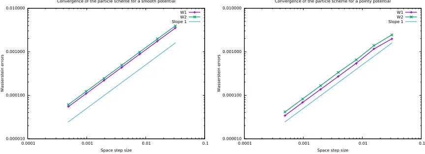
On Figure 3, one can see the convergence curves obtained for the two potentials.
0.000010 0.000100 0.001000 0.010000
0.0001 0.001 0.01 0.1
W
a
ss
e
rs
te
in
e
rr
o
rs
Space step size
Convergence of the particle scheme for a smooth potential
W1 W2 Slope 1
0.000010 0.000100 0.001000 0.010000
0.0001 0.001 0.01 0.1
W
a
ss
e
rs
te
in
e
rr
o
rs
Space step size
Convergence of the particle scheme for a pointy potential
W1 W2 Slope 1
Figure 3. Order of convergence of the particle scheme for the smooth potentialW(x) =x2/2
(left) and for the pointy potentialW(x) =|x|(right).
Theorem 2.1 states a convergence order for the particle scheme of 1/2 in time and 1 in space for the Wasserstein
distance d2. For the simulations, we choose a time step of the same order as the space step, meaning that an
order 1/2 is expected numerically. The results clearly show a better order. For both potentials and both
distances, the order is 1. This suggests that our estimate in Theorem 2.1 might not be optimal, at least for smooth initial conditions.
3.2.
Finite volume scheme: illustration of Theorem 1.2
The one dimensional problem presented here consists in two Dirac masses of weight 0.5 at a distance of 1
from each other at initial time. We are again considering the pointy and the smooth potential of Section 3.1:
(1) for the pointy potential W(x) = |x|, given the initial condition, the exact solution can be computed.
The two Dirac masses move toward each other, both at constant velocity 0.5, to merge at time 1 and
form a single Dirac masse with a weight of 1.
(2) for the smooth potential W(x) = x22, the exact solution is also known. The two Dirac masses move
toward each other but will never merge. The distance between the two Dirac masses is indeede−t in
this case.
We consider the domain [−0.75,0.75] and set the two initial masses at the points −0.5 and 0.5. Following
the notation of Section 1.4, the valuesρ0
J are thus all zeros, except for the two cellsJ− andJ+ containing the
points−0.5 and 0.5 respectively. For these two cells, we setρ0J− =ρ0J
+ = 0.5/∆x. Using the expression of the
velocity given by (14) and the upwind scheme of (13), we compute both the Wasserstein distances d1 and d2
To study the convergence order of the upwind scheme, we run, for the two potentials, several simulations
with a number of discretization points of 2k forkin the set {6, . . . ,12}. Because the exact solution is known,
we compute the Wasserstein errors with respect to this exact solution.
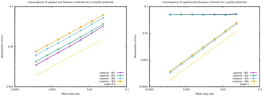
Figure 4 shows the results obtained for the two Wasserstein distancesd1andd2.
0.0001 0.001 0.01 0.1
0.0001 0.001 0.01 0.1
W
a
ss
e
rs
te
in
e
rr
o
rs
Mesh step size
Convergence of the upwind scheme for a smooth potential
W1 W2 slope 0.5 slope 1
0.0001 0.001 0.01 0.1
0.0001 0.001 0.01 0.1
W
a
ss
e
rs
te
in
e
rr
o
rs
Mesh step size
Convergence of the upwind scheme for a pointy potential
W1 W2 slope 0.5 slope 1
Figure 4. Order of convergence for the smooth potential W(x) = x2/2 (left) and for the
pointy potentialW(x) =|x|(right).
The numerical order of convergence in the case of the smooth potential is rather clearly 0.5 for both d1
and d2. Recalling estimate (17) of Theorem 1.2, this is the expected result in distance d2. However, for the
non-smooth pointy potential, it seems that we recover a first order of convergence. This difference can be explained by how two close Dirac masses interact with each other through the potential. Indeed, the velocity depends on the gradient of the potential. For the smooth potential, when two masses are close to each other, this gradient is close to zero. Compared to the numerical diffusion of the scheme, the agregation phenomenon
is less important and the order 0.5 is obtained. On the contrary, the pointy potential has a constant gradient
that does not depend on the distance between the two masses. Even at close range, the agregation phenomenon is important in this case. Moreover, it is acting as the opposite of the numerical diffusion and counter balanced it. This seems to lead to a better order of convergence (what would need a rigorous proof). Note that the link
with the Burgers equation with decreasing initial datum when the potential is |x|, made in [27], makes it clear
that this superconvergence phenomenon is linked with the same superconvergence for the Burgers equation with standard finite volume schemes, see [20], and also [34] for the viscous Burgers equation.
4.
Numerical results on unstructured meshes in dimension 2
It has already been proved and numerically checked that the upwind scheme (13) converges on Cartesian meshes for these aggregation equations (see [18]). It is easy to extend this result to another diffusive scheme such as the Rusanov scheme. We are interested here in their behaviors when used with non-Cartesian meshes. We first recall briefly the definition of the upwind and finite volume schemes on general meshes, for more
details we refer to [25]. Let us consider an admissible finite volume mesh of Rd denoted T (see Definition 6.1
in [25]). For an element K ∈ T, we denote |K| the measure of K and V(K) the set of its neighbours. For
L∈ V(K), we denoteL∩Kthe common interface betweenKandLand byνKLthe unit normal oriented from
We introduce the following explicit in time finite volume scheme
ρnK+1 =ρnK− ∆t |K|
X
L∈V(K)
|L∩K|g(ρKn, ρnL, νKL). (27)
This scheme is initiated by the conditionρ0K = |K1|RKρini(dx). The function g allows to define the numerical
flux. In this part we will consider the two following numerical methods :
• Rusanov
g(ρnK, ρnL, νKL) =
1
2(ρ
n
KanK·νKL+ρnLanL·νKL+a∞(ρnL−ρnK)). (28)
• Upwind
g(ρnK, ρnL, νKL) = (anK·νKL)+ρnK−(a n
L·νKL)−ρnL.
We use a two dimensional version of the toy problem of Section 3 to evaluate the numerical order of conver-gence. The triangular mesh is made of one line of squares, all cut in two along the same diagonal. Thus, the
domain is the set [−0.75,0.75]×[−∆x,∆x], where ∆xis the mesh step size. The initial condition is the same as
in Section 3. We identify the two cellsJ− andJ+whose center is the closest to the points (−0.5,0) and (0.5,0)
respectively. For these two cells, we setρ0J−=ρJ0+ = 0.5/A, where Ais the area of a cell. Everywhere else, the
initial condition is zero. The exact solution remains the same as this problem is essentially a one dimensional problem.
Considering again the pointy and the smooth potential, we run the simulations for several mesh step size and
compute both the Wasserstein errorsd1andd2. In order to compare these results, we run the same simulations
with the Rusanov scheme. Figure 5 shows the results obtained with the two schemes.
0.001 0.01 0.1
0.0001 0.001 0.01 0.1
W
a
ss
e
rs
te
in
e
rr
o
rs
Mesh step size
Convergence of upwind and Rusanov schemes for a smooth potential
upwind - W1 upwind - W2 rusanov - W1 rusanov - W2 slope 0.5
0.0001 0.001 0.01 0.1
0.0001 0.001 0.01 0.1
W
a
ss
e
rs
te
in
e
rr
o
rs
Mesh step size
Convergence of upwind and Rusanov schemes for a pointy potential
upwind - W1 upwind - W2 rusanov - W1 rusanov - W2 slope 1
Figure 5. Order of convergence for the smooth potential W(x) = x2/2 (left) and for the
pointy potentialW(x) =|x|(right).
In the case of the smooth potential, the schemes behave nicely and we recover the order 0.5 that we had in
the one dimensional setting. Concerning the pointy potential, however, some remarks are necessary:
(1) The upwind scheme seems not to converge to the correct solution, while the Rusanov scheme does. The solution with the upwind scheme is not blowing up but the velocity at wich the two Dirac masses are getting close to each other is higher than the exact one. Some tests have been run to understand precisely the reason of this non-convergence but no convincing results have been reached.
References
[1] J.-P. Aubin, A. Cellina,Differential inclusions. Set-valued maps and viability theory, Grundlehren der Mathematischen Wis-senschaften [Fundamental Principles of Mathematical Sciences], 264, Springer-Verlag, Berlin, 1984.
[2] L. Ambrosio, N. Gigli, G. Savar´e,Gradient flows in metric space of probability measures, Lectures in Mathematics, Birk¨auser, 2005
[3] L. Ambrosio, S. Serfaty,A gradient flow approach to an evolution problem arising in superconductivity, Comm. Pure Appl. Math., 61 (2008), 11, 1495–1539.
[4] A. L. Bertozzi, J. A. Carrillo, T. Laurent,Blow-up in multidimensional aggregation equations with mildly singular interaction kernels, Nonlinearity, 22 (2009), 3, 683–710.
[5] A.L. Bertozzi, J.B. Garnett, T. Laurent,Characterization of radially symmetric finite time blowup in multidimensional ag-gregation equations, SIAM J. Math. Anal., 44 (2012), 2, 651–681.
[6] A.L. Bertozzi, T. Laurent, J. Rosado,Lptheory for the multidimensional aggregation equation, Comm. Pure Appl. Math., 64
(2011), 1, 45–83.
[7] S. Bianchini, M. Gloyer,An estimate on the flow generated by monotone operators, Comm. Partial Diff. Eq., 36 (2011), 5, 777–796.
[8] G.A. Bonaschi, J.A. Carrillo, M. Di Francesco, M.A. Peletier,Equivalence of gradient flows and entropy solutions for singular nonlocal interaction equations in 1D, ESAIM Control Optim. Calc. Var., 21 (2015), 2, 414–441.
[9] Y. Brenier, E. Grenier,Sticky Particles and Scalar Conservation Laws, SIAM J. Numer. Anal., 35 (2006), 6, 2317–2328. [10] J.A. Carrillo, A. Chertock, Y. Huang, A Finite-Volume Method for Nonlinear Nonlocal Equations with a Gradient Flow
Structure, Comm. in Comp. Phys., 17 (2015), 1, 233–258.
[11] J.A. Carrillo, M. DiFrancesco, A. Figalli, T. Laurent, D. Slepˇcev, Global-in-time weak measure solutions and finite-time aggregation for nonlocal interaction equations, Duke Math. J., 156 (2011), 2, 229–271.
[12] J.A. Carrillo, R. Eftimie, F. Hoffmann,Non-local kinetic and macroscopic models for self-organised animal aggregations, Kin. Rel. Models, 8 (2015), 3, 413–441.
[13] J.A. Carrillo, F. James, F. Lagouti`ere, N. Vauchelet,The Filippov characteristic flow for the aggregation equation with mildly singular potentials, J. Differential Equations, 260 (2016), 1, 304–338.
[14] J.A. Carrillo, R.J. McCann, C. Villani,Contractions in the 2-Wasserstein length space and thermalization of granular media, Arch. Rational Mech. Anal., 179 (2006), 217–263.
[15] R.M. Colombo, M. Garavello, M. L´ecureux-Mercier,A class of nonlocal models for pedestrian traffic, Math. Models Methods Appl. Sci., 22 (2012), 4:1150023, 34.
[16] K. Craig, A.L. Bertozzi,A blob method for the aggregation equation, Math. of Comp., 85 (2016), 300, 1681–1717.
[17] F. Delarue, F. Lagouti`ere,Probabilistic analysis of the upwind scheme for transport equations, Arch. Rational Mech. Anal., 199 (2011), 1, 229–268.
[18] F. Delarue, F. Lagouti`ere, N. Vauchelet,Convergence order of upwind type schemes for transport equation with discontinuous coefficients, J. Math. Pures Appl., 108 (2017), 6, 918–951.
[19] F. Delarue, F. Lagouti`ere, N. Vauchelet,Convergence analysis of upwind type schemes for the aggregation equation with pointy potential, hal-01591602 and arXiv:1709.09416.
[20] B. Despr´es,Discrete compressive solutions of scalar conservation laws, J. Hyperbolic Differ. Equ., 1 (2004), 3, 493–520. [21] Y. Dolak, C. Schmeiser,Kinetic models for chemotaxis: Hydrodynamic limits and spatio-temporal mechanisms, J. Math. Biol.,
51 (2005), 6, 595–615.
[22] E Weinan,Dynamics of vortex liquids in Ginzburg-Landau theories with applications to superconductivity, Phys. Rev. B., 50 (1994), 2, 1126–1135.
[23] R. Eftimie,Hyperbolic and kinetic models for self-organized biological aggregations and movement: A brief review, J. Math. Biol., 65 (2012), 1, 35–75.
[24] A.F. Filippov,Differential Equations with Discontinuous Right-Hand Side, A.M.S. Transl., 42 (1964), 2, 199–231.
[25] R. Eymard, T. Gallou¨et, R. Herbin, Finite Volume Methods, Handbook of Numerical Analysis, Vol. VII, 2000, 713–1020., Editors: P.G. Ciarlet and J.L. Lions.
[26] F. James, N. Vauchelet,Chemotaxis: from kinetic equations to aggregation dynamics, Nonlinear Diff. Eq. and Appl. (NoDEA), 20 (2013), 1, 101–127.
[27] F. James, N. Vauchelet,Equivalence between duality and gradient flow solutions for one-dimensional aggregation equations, Disc. Cont. Dyn. Syst., 36 (2016), 3, 1355–1382.
[28] F. James, N. Vauchelet,Numerical method for one-dimensional aggregation equations, SIAM J. Numer. Anal., 53 (2015), 2, 895–916.
[29] F. Lagouti`ere, N. Vauchelet,Analysis and simulation of nonlinear and nonlocal transport equations, Innovative algorithms and analysis, Springer INdAM Ser. 16, 265–288, Springer, Cham, 2017.
[30] A. Mogilner, L. Edelstein-Keshet, L. Bent, A. Spiros, Mutual interactions, potentials, and individual distance in a social aggregation, J. Math. Biol., 47 (2003), 4, 353–389.
[32] F. Poupaud, M. Rascle,Measure solutions to the linear multidimensional transport equation with discontinuous coefficients, Comm. Partial Diff. Equ., 22 (1997), 1-2, 337–358.
[33] F. Santambrogio, Optimal transport for applied mathematicians. Calculus of variations, PDEs, and modeling, Progress in Nonlinear Differential Equations and their Applications, 87. Birkh¨auser/Springer, Cham, 2015.
[34] T. Tang, Z.-H. Teng,Viscosity methods for piecewise smooth solutions to scalar conservation laws, Math. Comp., 66 (1997), 218, 495–526.
[35] G. Toscani,Kinetic and hydrodynamic models of nearly elastic granular flows, Monatsh. Math., 142 (2004), 179–192. [36] C. M. Topaz, A. L. Bertozzi, M. A. Lewis,A nonlocal continuum model for biological aggregation, Bull. Math. Biol., 68 (2006),
7, 1601–1623.
[37] F. Venuti, L. Bruno, N. Bellomo,Crowd dynamics on a moving platform: Mathematical modelling and application to lively footbridges, Math. Comp. Model., 45 (2007), 3-4, 252–269.