Ranking Aggregation Based on Belief Function Theory

(1)

PhD Dissertation

International Doctorate School in Information and Communication Technologies

DISI - University of Trento

Ranking Aggregation Based on Belief Function

Theory

Andrea Argentini

Advisor: Prof. Enrico Blanzieri Universit`a degli Studi di Trento

(2)

(3)

Abstract

The ranking aggregation problem is that to establishing a new aggregate ranking given a set of rankings of a finite set of items. This problem is met in various applications, such as the combination of user preferences, the combination of lists of documents re-trieved by search engines and the combination of ranked gene lists. In the literature, the ranking aggregation problem has been solved as an optimization of some distance between the rankings overlooking the existence of a true ranking. In this thesis we address the ranking aggregation problem assuming the existence of a true ranking on the set of items: the goal is to estimate an unknown, true ranking given a set of input rankings provided by experts with different approximation quality. We propose a novel solution called Belief Ranking Estimator (BRE) that takes into account two aspects still unexplored in ranking combination: the approximation quality of the experts and for the first time the uncer-tainty related to each item position in the ranking. BRE estimates in an unsupervised way the true ranking given a set of rankings that are diverse quality estimations of the unknown true ranking. The uncertainty on the items’s position in each ranking is modeled within the Belief Function Theory framework, that allows for the combination of subjec-tive knowledge in a non Bayesian way. This innovasubjec-tive application of belief functions to rankings, allows us to encode different sources of a priori knowledge about the correct-ness of the ranking positions and also to weigh the reliability of the experts involved in the combination. We assessed the performance of our solution on synthetic and real data against state-of-the-art methods. The tests comprise the aggregation of total and partial rankings in different empirical settings aimed at representing the different quality of the input rankings with respect to the true ranking. The results show that BRE provides an effective solution when the input rankings are heterogeneous in terms of approximation quality with respect to the unknown true ranking.

Keywords

(4)

(5)

List of Tables

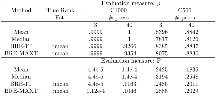
3.1 Spearman correlation coefficent (ρ) and Spearman Footrule distance (F) of BRE and of the competitor methods with respect to the true ranking.

means that BRE is significantly better than the corresponding

competi-tor, and means that BRE is significantly worse. . . 29

3.2 Average Spearman correlation coefficent (ρ) and Spearman Footrule dis-tance (F) of BRE and of the other competitors with respect to true ranking for the good, equal and poor cases with N = 10, 30 . . . 30 3.3 Spearman correlation coefficient (ρ) and Spearman Footrule distance (F)

of BRE using the mean and the raw mean as true-rank estimator. means

that BRE with mean is significantly better than BRE with raw mean as true-rank estimator . . . 32 3.4 Results of BRE with respect to the median and the mean on the video

datasets. Performance are evaluated in terms of ρ and F distances with respect to the true ranking. . . 34 3.5 Absolute and relative errors between the weights provided by BRE-1T and

QBRE with respect to the true weights. The statistical significance of the QBRE results with respect to BRE-1T is denoted by . . . 37

3.6 Results of BRE-1T with the different weighting schemas on the synthetic data. Performance are evaluated in terms of ρ and F distances with re-spect to the true ranking. The statistical significance of the base weighting schema with respect to all the other schema is denoted by , instead of that means the opposite case. . . 39

3.7 BRE with QBRE Weights vs BRE: Average ρ and F distance of BRE-1T with the weights evaluated on the synthethic data. The statistical signif-icance of BRE -1T (QBRE Weights) with respect to BRE -1T is denoted as , instead of that means the opposite case. . . 41

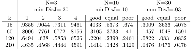
4.1 AverageDisJ coefficients on the 10 replicas for all the cases generated and the different k values. The lowest value (_N1) for the values of N = 3,10,30 are respectively .3, .1, .03. . . 48 4.2 Top-k rankings: Average of the scaled Spearman footrule distance (s.F)

of BRE and of the competitor methods with respect to the true ranking.

means that BRE is significantly better than the mean, and means

(8)

For each case the average of the DisJ coefficent is showed. . . 53 4.4 Top-k rankings from partial lists: Averaqe s.F distance of BRE and of the

competitor methods with respect to the true ranking. For each case the average of the DisJ coefficent is showed. . . 55 4.5 Average Partiality Index (P.I) for the dataset 2007-agg and 2008-agg . . . 59 4.6 LETOR 2007-agg: Precision and NDCG results of the BRE NW for all the

bbas evaluated against the mean. . . 63 4.7 LETOR 2008-agg: Precision and NDCG results of the BRE-NW for all the

bba evaluated against the mean . . . 64 4.8 LETOR 2007-agg: Precision and NDCG results of the BRE for all the bba

and the distances evaluated against the mean . . . 66 4.9 2008-agg: Precision and NDCG results of the BRE 1T for all the bba and

distances evaluated with respect to the mean . . . 67 4.10 LETOR 2007-agg: Comparison of BRE and the mean in terms of NDCG

on all the partions evaluated . . . 72 4.11 LETOR 2008-agg: Comparison of BRE and the mean in terms of NDCG

(9)

List of Figures

3.1 Example of BRE with NW schema: BBA from rankings (Eq. 3.1), combi-nation (Eq. 3.5) and the ranking outcome (Eq. 2.13) . . . 22 3.2 Example of BRE with weighting schema: weight application (Eq. 3.4),

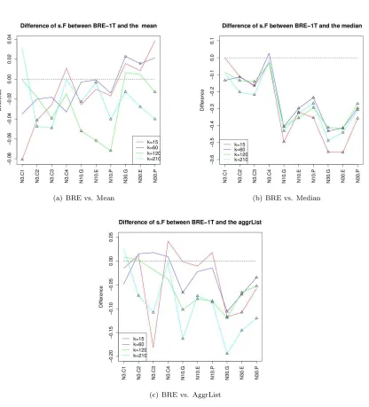
com-bination (Eq. 3.5) and the ranking outcome (Eq. 2.13)). The weights are computed using the mean of the rankings as true-rank estimator (Eq. 3.3). 24 4.1 Difference of s.F distance of BRE and the competitors. With△and are

highlighted respectively the cases where BRE outperforms significantly the competitors and BRE is outperformed significantly by the competitors. . . 50 4.2 BRE on Partial Rankings: Differences of BRE with respect to competitors

in terms of s.F distance. With △ and are highlighted respectively the

cases where BRE outperforms significantly the competitors and BRE is outperformed significantly by the competitors. . . 54 4.3 BRE on Top-k Lists of Partial Rankings: Differences of BRE with respect

to competitors in terms of s.F distance. With △ and are highlighted

respectively the cases where BRE outperforms significantly the competitors and BRE is outperformed significantly by the competitors. . . 56 4.4 The four bbas evaluated on LETOR, applied on a ranking with kj = 4

where the query contains Dn= 8 documents . . . 62 4.5 2007-agg: Result of BRE among the different BBA’s evaluated in terms of

NDCG . . . 64 4.6 2008-agg: Result of BRE among the different BBA’s evaluated in terms of

NDCG . . . 65 4.7 Histogram of NDCG@Mean obtained by the median in the 2007-agg and

2008-agg datasets. . . 69 4.8 2007-agg: Best results of BRE-1T with respect to the mean for all the

clusters evaluated . . . 70 4.9 2008-agg: Best results of BRE-1T with respect to the mean for all the

(10)

(11)

List of Algorithms

(12)

(13)

Chapter 1

Introduction

Ranking aggregation is a relevant problem that is faced in several application contexts such as marketing research, psychology and meta-search. In its general form the problem is stated as follows: given a set of experts or judges providing an ordered list from a set of items, the goal is to find a list that best represents the wholeset of input rankings according to some measure. A practical context that has given large in impulse to ranking aggrega-tion soluaggrega-tions is the so-called meta-search where the results of several search engines have to be combined to produce a consensus answer. Also in Bioinformatics, the aggregation of rankings emerges from the need to integrate different biological data related to the same question to be investigated. Although ranking aggregation is an optimization problem based on distance, it been shown that the solution of the Kemeney optimal aggregator (with Kendall’s distance) is an NP-hard problem even with justfour rankings. This com-putational limitation has led to several solutions to alleviate the comcom-putational burden of the problem. The ranking aggregation methods can be divided into two groups, one which comprises stochastic optimization methods and the other that includes heuristic methods. The methods in the first group try to find the best aggregated ranking using an optimization method, whereas the heuristic methods approximate the solution by means of heuristics. The rankings can be divided into three kinds: total rankings, partial and top-k rankings (lists). The difficulty of the aggregation is greater in the case of partial or top-k lists since the lists have different lengths and share also disjoint sets of items. We point out that in the formulation of the ranking aggregation problem the quality of input rankings and the presence of a true ranking is overlooked. Few works in literature have arisen this fact, highlighting that the ultimate goal is to find an aggregate ranking closer to the true ranking. In this work we tackle the ranking aggregation problem intro-ducing the true ranking in its formulation. The goal is to find a satisfying estimatate of the unknown true ranking given a set of input rankings provided by experts with different degree of approximation quality. We claim that this the case for rankings provided by bioinformatic experts because of the underlying physical reality of the unknown biological phenomenon at hand.

(14)

allowing the modeling of subjective knowledge in a non Bayesian way. Given a frame of possible hypotheses or items, the framework allows us to assign a quantitative measure of the expert evidence on the whole power set of the frame. This leads to model vari-ous levels of knowledge of the experts from complete knowledge down to total ignorance. Several combination rules and conditioning operations are defined in the framework, to update and combine the beliefs of the experts. Moreover, the framework extends both the usual set theory operations (union, intersection) and probability theory (condition-ing, marginalization). The Belief Function Theory has been applied to machine learning problems such as classification, clustering and combination of classifiers.

In this thesis we propose and evaluate a novel algorithm, called Belief Ranking Estimator (BRE) that estimates the true ranking given a set of rankings. Through the use of Belief Functions we model the correctness of the items ranked from the point of view of each expert (ranking): we then combine all the experts views taking into account the reliability of the rankings involved. The reliability of the input rankings is assessed by computing the distance at the rankings to a true-rank estimator. As the true-rank estimator we can to use the output ranking of any aggregation method.

The novelty of our solution lies in a new formulation of the ranking aggregation problem that takes into account the quality of the input rankings with respect to the true ranking. A second aspect is the modeling of the correctness of the rank in order to manage the uncertainty of the items ranked, using Belief Functions. To the best of our knowledge this framework has never been applied to ranking aggregation before. Moreover, this is the first approach in the ranking aggregation literature that deals with the uncertainty of ranked items. One of the aadvantages is that our approach alloes to model different pieces of a priori knowledge about the experts involved (such as the correctness of the positions of a subset of the items with respect to the others) into the aggregation step. Several possible extensions of the algorithm may be proposed. We have focused our efforts on the empirical results of our method instead of pursuing a more theoretical analysis. The performance of our solutions has been compared against state-of-the-art methods, on both synthetics and real data. With respect to total rankings, we have evaluated the per-formance of BRE using different true-rank estimators. Moreover, the role of the weights in the algorithm has been deeply investigated. A novel algorithm, called Quality Belief Ranking Estimator (QBRE), for the approximation of the quality of the input rankings has been proposed and evaluated on total rankings. Due to the lack of real data containing total rankings with an available true ranking, we have developed a rigorous experimental setting based on synthetic data. On the partial/top-k rankings we have investigated the performance of BRE both on the synthetic data and on real data. On synthetics data we have tested BRE on three cases of partial rankings that meet different hypotheses on the quality of the experts. Finally, BRE has been evaluated on LETOR, that is a collection of datasets related to the meta-search problem.

(15)

one of key points in our solution. Weights that are good estimation of the quality of the input rankings increase considerably the performance of BRE. The evaluation of BRE on partial/top-k rankings has highlighted some difficulties to outperform the competitors. As for partial rankings, we have also showed how BRE can encode different a priori in-formation such as different belief assignments.

(16)

(17)

Chapter 2

Ranking Aggregation and Belief

Functions: An Introduction

2.1

The Ranking Aggregation Problem and its Application

Ranking aggregation is a well-studied problem, that arises in different areas such as psychology, market advertisement research, combination of experts in Information Re-trieval or in Bioinformatics. Rankings speaking generally, are ordered sets of items where the order can be provided in several ways: for example, from the subjective preference of users or from the output numeric score of an algorithm (e.g. a classifier). The problem of ranking aggregation concerns the combination of several rankings in order to obtain a final ranking that satisfies specific criteria.

The ranking is a really simple structure that encodes in a intrinsic way some of the knowl-edge that brings on expert or an user to generate an ordered list. On the other hand, the hidden information that has generated the ranking is really difficult to know and use in the aggregation step. For this reason ranking aggregation methods are based only on the information of the rankings: the items and their position. Rankings are defined as total if they are permutations of the set of items. In many situations, rankings are partial: not all the lists contain the same items. A particular case of partial lists are top-k lists, where only the first k items are included in the rankings. However, in most of the real applications (for example document meta-search) partial/top-k lists are the only rankings available, and the partiality of the rankings increases the difficulties of the aggregation task.

(18)

condition [1]. Other Bioinformatics tasks where ranking aggregation has been applied are the combination of miRNA target prediction and the combination of different gene expression microarray studies [2]. Ranking aggregation has also been widely applied to the meta-search problem, which concerns the combination of the answers of several web search engines [3][4][5].

Statistics has given a notable contribution to the study of distances between rankings [6] and of probabilistic models able to deal with the combination of rankings, such as Thurstone’s model[7][8], Luce’s model [9][10], and Mallow’s model with its extension to partial data [11][12][13]. The solutions provided for the ranking aggregation problem are basically of two categories: Stochastic optimization and heuristic methods. In the first category, optimization techniques, such as cross-entropy Monte Carlo [2][14] and genet-ics algorithms [15], are applied to obtain the optimal aggregation for a given distance measure. Heuristic methods are simpler methods that find a solution based on their own criteria, such as the Borda Count’s methods that include the mean and the median of the rankings [16][4], the Markov Chain [4] and MEDrank [17]. Moreover unsupervised and supervised algorithms based on generative models for rankings have been applied to ranking aggregation on meta-search problems [5][18][19].

In the following section we briefly define formally the rankings and the major distances used in rankings aggregation. Sec. 2.3 is devoted to the presentation of the state-of-the-art solutions for aggregating rankings. Finally, we introduce a slightly different point of view on ranking aggregation based on by the presence a true ranking underlying the real situation.

2.2

Definition of Rankings and Distance between Rankings

Before describing the ranking aggregation problem and the different types of solutions proposed in literature, we introduce and define the rankings and the most used distances between them. We begin with total rankings, ranking is a permutation of a set of objects.

Let X = {x1, . . . , xn} be a set of items to be ranked by an expert opinion. We refer

indistinctly to the objects inX as elements or items. We denote asτ = (τ(1), . . . , τ(n)) a ranking associated to X, where τ(i) is the rank associated with the item xi. Each expert

knows all the elements in X, and it provides an ordering of its elements. We denote as

Rj the j-th expert involved in the ranking, so for each expert we have a corresponding

ranking τRj _{= (}_τRj₍₁₎_{, . . . , τ}Rj₍_n_{)). To simplify the notation, each ranking is denoted by}

τj _{for all}_j _∈_N _where_N _{is the number of experts and consequently of rankings. The rank}

values associated to the most important element can be either 1 or n, without any loss of generality in the permutation case. The notation |τj_| _{means the length of the ranking}

and in case of total rankings for all j ∈N n=|τj_{|. We point out that for sets specified}

with {}the ordering of the elements is arbitrary, whereas when using (), a specific order with respect to the rank of the items is given.

(19)

2.2. Definition of Rankings and Distance between Rankings

values of the rankings. We define the footrule distance as follows:

F(τ, σ) =

n

X

i=1

|τ(i)−σ(i)| (2.1)

where τ and σ are total rankings. As indicated in [6], the F distance can be normalized by dividing by the maximum value n₂2, so that an F value equal to 1 means totally differ-ent rankings and 0 means iddiffer-entical rankings. TheF distance is computable in linear time. The Kendall distance [20] compares rankings, counting the pairwise disagreements between two rankings. Formally, Kendall’s distance [21] between two total rankings τ

and σ is defined as:

K(τ, σ) = X

{i,j}∈P

K_i,j∗ (τ, σ) (2.2)

whereP is the set of the unordered pairs of distinct items in X and K∗

i,j(τ, σ) is defined

as:

K_i,j∗ (τ, σ) =

(

0 ifxi, xj are in the same order inτ andσ

1, if xi, xj are in the inverse order inτ andσ

(2.3)

Kendall’s distance can be normalize by dividing by its maximum value n₂

[6]. It turns out to be the number of adjacent transpositions needed to transform one ranking into the other and it can be computed in nlogn time.

Another measure to evaluate correlation between two rankings is Spearman’s rank cor-relation coefficent [20][22]. Given two total rankings τ and σ, Spearman’s correlation coefficent, denoted byρ, is defined as :

ρ(σ, τ) = 1− 6

Pn

i=1(π(i)−σ(i))2

n(n2₋₁₎ (2.4)

ρis defined as the Pearson correlation between two ranked variables, namely rankings. ρ

returns values in the interval [−1,1]. ρ= 1 means a total positive correlation between the rankings instedρ=−1 means a total negative correlation between the input rankings.

If the items present in the rankings are not the same, two different situations can arise: Partial rankings and top-k rankings. Partial rankings, also referred to as partial lists, occur when the rankings are induced by a total ordering over a subset ofX. We denote as

τj _{= (}_τj₍₁₎_{, . . . , τ}j₍_i₎_{, . . . , τ}j₍_l

j)) the partial ranking of lengthlj =|τj|, where Cj denotes

the set of items in thej-th ranking andxi ∈Cj, Cj ⊂X. This situation is really common

in real problems, for example in meta-search applications, search engines return a list of documents for a query that contains a far fewer of documents than the number of all web pages. In this case we cannot make any assumption for the documents not ranked by the expert, since the relation between the subset of items and the universe setU is unknown. Top-k rankings are a special case of partial rankings for which only the top k elements are included in the output rankings of the experts. The top-k rankings are still denoted

by τj _{= (}_τj₍₁₎_{, . . . , τ}j₍_i₎_{, . . . , τ}j₍_l

j)), with length of kj = lj = |τj| and xi ∈Cj, Cj ⊂ X.

(20)

the unranked items in a top-k list can be placed below, with the same rank values. A detailed description of the hypothesis evaluated on partial ranking/top-klists is discussed in Chapter 4

To deal with the comparison between partial rankings and total rankings, a suitable generalizations of the distances on total rankings are to be defined. We denote as τ|S the

projection of a ranking τ with respect to a subset S this produces a new ranking that contains only the element in S and maintains the order of τ.

Induced Footrule Distance Given τ1_{, . . . , τ}N _{partial rankings, let} _U _{be the union of}

the elements in τ1_{, . . . , τ}N _and _σ _{a total ranking w.r.t} _U_{. The induced footrule distance}

[4] between σ and a partial list τj _is:

i.F =F(σ|τj, τj) (2.5)

where the σ|τj is the projection of the total ranking σ on the elements of the partial

ranking τj_{. In this case the result} _σ

|τi is re-ranked in order to compute the F distance.

The normalization of the i.SF is done dividing by |τ₂j|2, since it is anF distance computed on the same items. In case of N partial rankings the induced footrule distance is:

i.F(σ, τ1, . . . , τN) =

N

X

j=1

F(σ|τj, τj)

N

Scaled Footrule Distance The scaled footrule distance [4] is defined as follows:

s.F(σ, τ) = X

i∈Cτ

|σ(i)/|σ| −τ(i)/|τ|| (2.6)

where σ, τ are respectively the total ranking and the partial ranking and Cτ is the set of

elements ranked in τ. The main difference between the scaled one with respect to the induced version, is the weighting of the distance based on the size of the rankings. We have normalized the s.F distance dividing by |τ|/2 as suggested in [4]. We presented only the distances related to the Spearman footrule distance since we deal only with this distance in this work. For Kendall distance versions for partial and total rankings have also been proposed [21]. An easy way to manage and compare top-k rankings is to transform the top-krankings in a sort of total rankings (so-called augmented rankings [5]) where in each list the unranked items are placed at position k+ 1 and finally apply the usual distances.

2.3

Ranking Aggregation Methods

In this section we provide a discussion of state-of-the-art methods and a formal defini-tion of the ranking aggregadefini-tion problem.

(21)

2.3. Ranking Aggregation Methods

on the set of itemsX, the goal is to find the underlying order onX, τ. Suppose that the input rankingsτj _{are noisy versions of}_τ_{, obtained by swapping two elements of} _τ _{with a}

probability p < 1/2. The maximum likelihood estimate of τ using the Kendall distance

K is [23]:

τ∗ = arg min

τ

1

N

X

j=1

K(τ, τj) (2.7)

The estimate τ∗ _{is referred as to Kemeny optimal aggregation [4]. Dwork} _{et al.} _have

shown that the computation of the Kemeny optimal aggregation is a NP-hard problem even when the number of rankings is four [4]. In order to solve the Kemeny optimal aggregation-problem, stochastic search solutions and heuristic solutions has been pro-posed.

The Kemeny optimal aggregation (Eq. 2.7) can be approximated via the Spearman footrule distance [4]. This leads to the Footrule optimal aggregation where the above optimal aggregation criteria is based on the Spearman footrule distance. The Footrule optimal aggregation for total rankings is computable in polynomial time by reduction to the computation of the minimum cost of matching on weighted bipartite graph [4].

Let τ1_{, . . . , τ}j_{, . . . , τ}N _be _N _{total rankings over a universe set} _X ₍_n ₌ _|_X_{|). We define}

a weighted bipartite graph (X,P,W), where X = {xi, . . . , xn} is the set of the items to

be ranked and P = {1, . . . , n} contains the n possible positions p ∈ P. Each node of

X is connected to all the possible positions. The weight for each edge W(xi, p) is set

to the total footrule distance of the rankings that rank item xi item at position p. This

corresponds toW(xi, p) = N

X

j=1

F(τj(i), p). The output is the permutation over the set X

that results by the minimum cost of perfect matching in the bipartite graph.

In the case of partial lists, finding the Footrule optimal aggregation is an NP-hard prob-lem, Dwork et al. suggest to solve the problem (as in the case of total rankings) as the minimum cost of a bipartite graph in which the weights assigned are based on the scaled footrule distance [4].

Stochastic Optmimization

In order to efficiently explore the combinatorial solution space to find the τ∗ _from

(22)

Chain solutions [2]. It has also been applied in another bioinformatics work where the task was to find the best clustering algorithms across different evaluation measures space [14]. In that work it has been introduced a weighted formulation of both the footrule and Kendall distances. The weights used are the quantitative outputs of the methods (scores), in order to penalize the difference of the rank of each item. The same authors have implemented the CEMC algorithm in a R package called RankAggr [15]. In the same work an optimization algorithm based on genetic algorithms is also proposed.

Heuristic Solutions for Ranking Aggregation

Methods which provide approximate solutions without optimizing any cost function, are classified as heuristic. This category include the Borda Count [16][4], the MEDrank algorithms, and also other simple heuristics such as the median and the mean of the rank-ings that can be generalized by the Borda Count.

Borda Count is a really simple method that can include different aggregation functions. Borda Count assigns to each item xi a score B(i) corresponding to the position in which

the item appears in a specific ranking. For each item all the scores are summed up for all the rankings and finally the items are ranked by their total score. Given N

total rankings τ1_{, . . . , τ}j_{, . . . , τ}N _{for each item} _x

i ∈ X and for each ranking τj Borda

Count assigns a score Bj₍_i_{) equal to the number of items placed below} _x

i in τj. Let

Bi = f(B1(1), . . . , Bj(i), . . . , BN(n)) an aggregate function of the Borda scores where

i ∈ {1, . . . , n,} the final rankings is obtained sorting the Bi score. The most used

aggre-gate functions [1][4] are:

– the median f(B1_{, . . . , B}N_{) =}_median₍_B1_{, . . . , B}N₎

– the geometric mean f(B1_{, . . . , B}N_{) =} N

Y

l=1

Bl

!1/N

– the p-norm f(B1_{, . . . , B}N_{) =} N

X

l=1

(Bl)p

We point out that the arithmetic mean is a special cases of the p-norm when p= 1 and

Bj₍_i_{) =} _τl₍_i_{). In the case of partial rankings the Borda Count works as in the total}

ranking case, the only difference is that an equal score is assigned to the unranked items for in each partial ranking.

Another heuristic proposed to solve the Kemeny optimal aggregator is based on Markov Chains space [4]. Borda Count methods consider the rankings in their totality, whereas Markov chains allows to model pairwise ranking information. All the items presented in the rankings (or in the union in case of top-k lists) are represented in a graph, where the transition probabilities from one node xi to another nodexj encode the pairwise ranking

(23)

2.3. Ranking Aggregation Methods

approach, in fact four Markov Chain schema (named MC1, MC2, MC3, MC4) has been proposed in [4] and each one uses a different heuristic. Without describing the details of each MC schema, the most interesting for the partial ranking is MC4, where the initial transition matrix gives an high probability value to a move from the state P to the state Q if in the majority of the rankings the items P is ranked above Q. Being heuristic none of the proposed Markov chains methods produces a Kemeney optimal aggregation, but they show interesting performances in practice. [4]. Other Markov chains methods for ranking aggregation has been proposed also in [1], in order to best suit the bioinformatics applications.

Among the heuristic methods, there is also the MEDrank algorithm [17] that is based on the idea of aggregating the input rankings using a median rank for each item. MEDrank in the case of total rankings can optimize the Footrule optimal aggregation if the aggregate ranking has no ties. Moreover, MEDrank satisfies also the Kemeny optimal aggregation within a constant bound (see. [4]). The algorithm is described as follows. Given N total rankingsτ1_{, . . . , τ}j_{, . . . , τ}N _{defined over a set}_X ₌_{_{x1, . . . , x}

i, . . . , , xn}of items, letc(i, φ)

a function that returns the number of rankings for which τ(i) = φ. At the beginning a rankM(i) = 1, i∈X is assigned to all the items. The algorithm starts with φ = 1, and at each step it updates for all the items theM(i) asM(i) =M(i) +c(i, φ). The first item that reaches M(i)> β gets a rank value equal to 1 in the output list and it is no more considered. The second item that reaches the same condition gets rank 2 an so on until all the rank values up to φ are assigned to the items. The suggested value of threshold

β is N₂: an item must be counted at least a numebr of times equal to half the number of input rankings before being placed in the aggregate ranking. In the case of top-k lists, MEDrank terminates when the number of items in the aggregate ranking reaches k.

Probabilistic Models for Ranking Aggregation

(24)

Mallow’s model is based only on the ranking distance. In order to overcome the limitations and inherit the expressiveness of the two models, a novel probabilistic model called coset-permutation distance-based stagewise model (CPS), has been proposed and evaluated on a ranking aggregation task based on a meta-search problem [19]. The latter is a supervised algorithm that learns the parameters of the CPS model using a training set of rankings, after which an inference step produces the results on a test set.

2.4

Related Works: Learn to Rank Problem

Another issue related to rankings is the learn-to-rank problem. Here the goal is to learn a ranking model from training data. Learn to rank solutions are widely applied to the meta-search problems [3], where the goal is to learn a ranking function that orders the query-documents on the base of their relevance. Two well-known algorithms, based on a pairwise approach are RankBoost [24] and RankSVM [25]. For a complete review of the problem and the algorithms proposed we refer to a specific work [26]. The main difference between the learn-to-rank problem and ranking aggregation is the use of a training set to learn the rank model. This training set includes the rankings but also the relevance values associated with the items. Moreover, in meta-search problem the training data contains also a vector of numeric features relative to the query-document pairs [3]. The ranking aggregation methods presented above do not use relevant labels on the items but only rankings and they do not admit a learning step (expect for the probabilistic models). The ranking aggregation methods presented are total unsupervised solutions in fact no training rankings are available, thus it is not possible to compare the performance of this two approaches.

2.5

Ranking Aggregation vs. The Estimation of True Ranking

As mentioned above, in ranking aggregation the problem is to find a ranking that minimizes the distance from the input rankings. In this work, we deal with ranking aggregation from a point of view that is slightly different from the methods presented in our review of the state of the art. We have noted that the quality of input rankings with respect to a “true ranking´’ and also the existence of the true ranking is not taken into account in the ranking aggregation problem.

The relation between ranking aggregation methods and true ranking has been investigated in [27], where several ranking aggregation methods are compared in order to measure how the quality of the input rankings impacts the performance of the aggregate rankings. The author has showed with rigorous experimental evaluation that the performance of different aggregation methods is deeply connected to the extend whith which the input rankings are related to the true ranking.

(25)

2.6. Belief Function Theory

predictors in order to find a consensus list that contains in the first positions the true positive targets. A true ranking exists, but we know only a dichotomous ranking where items should be in top positions if they are true targets, or in the later part of the ranking otherwise [28]. Inspired by these considerations, we tacke the ranking aggregation problem by assuming the presence of a true ranking on given a set of items. The goal is to find a satisfying estime of the unknown true ranking given a set of input rankings provided by experts with different ”approximation quality¨. The main difference with respect to the ranking aggregation solutions based on minimization criteria is that we assume that the true ranking over the set of items does exist. Since we do not search a consensus list from the input lists, our approach does not address the ranking aggregation of user preferences.

2.6

Belief Function Theory

The Belief Function theory provides a robust framework for reasoning with imprecise and uncertain data, allowing the modeling of subjective knowledge in a non Bayesian way. The theory of the Belief Functions, also known as Dempster-Shafer theory, is based on the pioneering work of Dempster [29] and Shafer [30]. More recent advances of this theory has been introduced in theTransferable Belief Model (TBM), proposed by Smets [31]. The Belief Function Theory is a powerful framework to deal with decisions in all the situations where data is imprecise and the subjective views is an important features such as in information fusion tasks. Belief Functions theory generalizes both Set theory (intersection, union) and Probability theory (marginalization, conditioning). The TBM framework is divided in two levels, thecredal level is where the belief is assigned to a set of possible choices and this belief is updated and combined through several operators, and thepignistic level where decisions are taken on the set of choices. In the next sections we provide a basic explanation of the framework through the most common operators and a brief discussion of the application of belief functions on machine learning tasks.

2.6.0-A Representation of Evidence

We define Θ ={θ1, . . . , θk}as a set of propositions about the exclusive and exhaustive

possibilities in a certain domain. Θ is called the frame of discernment. Let 2Θ _{denote the}

set of the possible subsets of Θ. A functionm: 2Θ _→_[0_,_{1] is called}_{basic belief assignment}

(bba) if it satisfies:

m(∅) = 0 X

A⊆Θ

m(A) = 1

(26)

combination of several experts, the other is that the expert (or the combination of the experts) has belief in an hypothesis outside the frame Θ. The modeling of the ignorance of an expert lies in the possibility to assign evidence to a set of elements instead of assigning it to just a single element. If Θ = {a, b} and in the case the expert does not have any prior knowledge, m({a, b}) = 1 represents the total ignorance or confusion of the expert to decide between the two events. In the probability framework the uncertainty could be modeled using a prior over the events. In the previous example the ignorance/confusion could be modeled as P(a) =P(b) = 0.5 where the two propositionsaand bhave the same prior probabilities. It is easy to recognize the differences of the two approaches respect to the modeling of the uncertainty. In the probability model we have probability values for the two propositions whereas in the Belief Function framework the model directly repre-sents the total ignorance over the pair of propositions without any additional assumption. Some of the possible bbas are:

Bayesian All focal elements are singletons (Θ ={a, b}, m(a), m(b)>0)

Simple The bba has two focal sets and one of those is Θ (Θ = {a, b}, m(a) > 0 and

m(Θ) >0)

Categorical The bba has only one focal set (Θ ={a, b}, m(a)>0) Vacuos The bba has only m(Θ) = 1 as focal set.

If m is a valid bba ove the frame Θ, then the belief function Bel : 2Θ _→ _[0_,_{1] is defined}

as:

Bel(A) = X

B⊆A

m(B)

Another notion introduced in this framework is the plausibility function. P l : 2Θ _→_[0_,_1]

defined as:

P l(A) = X

A∩B6=∅

m(B)

It is also possible to express the plausibility asP l(A) = X

A∩B6=∅

m(B). The quantityBel(A) is the degree to which the evidence supports A, whereas theP l(A) is the upper bound of the degree of support that could be assigned on A. Moreover, it is possible to obtainm

from the Bel via the following trasformation:

m(A) =





 X

∅6=B⊆A

(−1)|A|−|B|

Bel(B) A6=∅

1−Bel(Θ), A=∅

(2.8)

(27)

2.6. Belief Function Theory

2.6.0-B Combination and Updating the Belief

In order to aggregate distinct sourcesm1, . . . , mnon Θ, the framework provides several

combination rules, such as the conjunctive rule, the disjunctive rule and the caution rules [31] among others. The conjunctive rule is defined as:

m1O∩2(A) =

X

B∩C=A

m1(B)m2(C) A ⊆Θ (2.9)

The conjunctive ruleO∩ is justified when all the sources of belief are supposed to assert the

truth and to be independent. Moreover,m1O∩2(∅) represents the degree of conflict between

the two bbas. Conflict arises when the different sources have singleton focal elements, in which case their intersection is∅. Another conjunctive operator isDempster’s combination rule, defined as:

m1⊗2(A) =



 

 

X

B∩C=A

m1(B)m2(C)

1−K A 6=∅

0 A =∅

whereK is the degree of conflictm1O∩2(∅): the⊗operator the conflict is used to normalize

the combined bbas. The conflict in the belief function framework can have different meanings and it should be managed in accordance to the application at hand. One possible meaning is that the frame Θ is not exhaustive, andm1O∩2(∅) quantifies the belief

that there exist hypothesis θ outside the frame Θ (open-word assumption). Otherwise

m1O∩2(∅) means that the sources do not report on the same object, this is applied in some

applications where the sources are clustered according to which object they report [32]. The use of the two conjunctive operators ⊗ and O∪ is related to the type of application.

The conjunctive operator is well indicated when we need to keep track of the conflict between the bbas to combine, wheres the⊗ rule is suggested when the conflict should be normalized.

If the sources to combine are still independent but at least one of the tells the truth (without knowing with one), then the disjunctive combination rule is more appropriate. Given two mass functionsm1 and m2 defined on Θ the disjunctive rule O∪ is defined as:

m1O∪2(A) =

X

B∪C=A

m1(B)m2(C) A ⊆Θ (2.10)

The disjunctive operator is associative, commutative and admits as neutral element the bba which assigns a total belief to the empty set (m(∅) = 1). In the literature other combination rules have been proposed such as the Debois and Prade’s rule [33] and the Yager’s rule [34]. These combination rules are a mix of the conjunctive and disjunctive operators, and propose other ways to deal with the conflict generated by the combination. Even if we do not present the details, we mention also the cautious rule [35], a combination rule appropriate when the sources of belief are dependent.

(28)

discount operation is defined as [36]:

m∗(A) =αm(A) A⊂Θ

m∗(Θ) = 1−α[1−m(Θ)] A= Θ (2.11) where m∗ _{are the discounted bbas. When decreasing} _α _{down to 0 the bba loses all its}

information, and the result is a vacuous belief functionm(Θ) = 1. A fully realiable source has α= 1, which leaves the bba unchanged. In case of simple bbas over a frame Θ defined as follows,

m(A) =s

m(Θ) = 1−s

m(B) = 0 ∀ 2Θ{Θ, A}

where m(A) is the only focal element except m(Θ), and s∈[0,1], the discount operation can be rewritten as:

m∗(A) =αs

m∗(Θ) = 1−αs (2.12)

2.6.0-C Decision Making

In the TBM framework the uncertainty reasoning is performed at the so-called credal level, where the bbas are combined and updates, instead the decision making is made at the pignistic level where the belief are used to make decision [31][37]. TBM framework to make decision requires to quantify the belief in probability in order to avoid the Dutch Books. Dutch Book is a set of bets that lead to a sure loss regardless of the outcome of the gamble. This only way to prevent this situation is to be certain that our belief is reppresented by a probability function. Smets proposes the pignistic transformation to transforms the masses defined on the power set of Θ to a probability space defined only on single atoms of Θ as following:

Betp(θ) = X

{A⊆Θ,θ∈A}

m(A)

1−m(∅)|A| ∀θ ∈Θ (2.13) The idea underling the pignistic transformation is to distribute equally every bba on the singleton elements that belongs to its focal element. Smets justifies the pignistic trasfor-mation as the only trasfortrasfor-mation that satisfies five specific assumptions related to the properties that the trasformation must satisfy. For a detailed description of all the as-sumptions satisfied by the pignistic trasformation we refers to [38]. Even if in this work we use the pignistic trasformation, other methods to map bbas into a probability measure such as the plausibility trasformation [39] has been proposed in literature.

(29)

2.7. Applications of Belief Function Theory

2.7

Applications of Belief Function Theory

(30)

(31)

Chapter 3

BRE: Belief Ranking Estimator

3.1

Introduction

(32)

unsupervised way given a set of input rankings. We evaluate BRE on total rankings of synthetic data and compare our method against some ranking aggregation competitor methods.

3.1.1 Notation and Definition of the Problem

LetX ={x1, . . . , xn} be a set of items to be ranked by an expert opinion. We denote

asτ = (τ(1), . . . , τ(n)) a ranking associated toX, whereτ(i) is the rank associated to the

item xi. We suppose to have τTrank = (τTrank(1), . . . , τTrank(n)), that is the golden ”true`‘

ranking on the items of X, and we denote asRj the expert involved in the ranking, so for

each expert we have a corresponding ranking τRj = (τRj(1), . . . , τRj(n)). To simplify the

notation, each ranking is denoted byτj _{for all}_j _∈_N _where_N _{is the number of experts and}

consequently of rankings. We suppose also that the most important items for a ranking

τj _{receives a rank value equal to}_n_{. This assumption in the set of the permutations does}

not lead to any loss of generality. The problem in its general form is stated as follows. Given N rankingsτRj _{of length}_n _{of the}_n_items _X₌_{_{x1, . . . , x}

n}, namely permutations,

that estimate with unknown quality the unknown true ranking τTrank find a ranking that

estimates the true ranking.

3.2

BRE: Belief Ranking Estimator

The Belief Ranking Estimator (BRE) is an unsupervised algorithm that iteratively computes an estimation of an unknown true ranking, given N input rankings that are assumed to be approximations of unknown quality of the true ranking. The core of the method is the use of belief functions in order to capture and model the uncertainty regard the position of each item contained in each ranking. Through the use of a true-rank estimator, BRE estimates the quality of the input rankings to use this information in the combination process. The main steps of the Belief Ranking Estimator are the following:

– Mapping the rank value of each item into belief assignments.

– Assessment of the quality of the input rankings using a true-rank estimator.

– Application of the quality information of the input rankings to the belief assignments .

– Combination of the beliefs associated with each item to produce a ranking as out-come.

(33)

3.2. BRE: Belief Ranking Estimator

Algorithm 1Belief Ranking Estimator: Iterative version

input I=τ1_{, . . . , τ}N _{// a vector of N Rankings}

input T // Numbers of iterations

input T E // True-rank estimator k= 0

BE=Belief From Rankings(I)

F inalRankk=Combination(BE)

while k !=T do

¯

w=ComputeWeights(I,TE(I)) BE=ApplyWeights( ¯w,BE)

F inalRankk=Combination(BE) I[pos(max( ¯w))]=F inalRankk BE=Belief From Rankings(I) k++

end while

output F inalRankk

3.2.1 BBA From Rankings

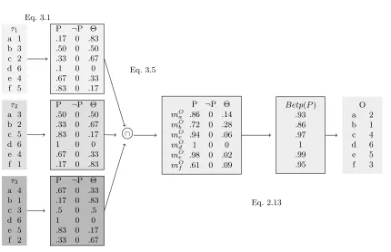
The mapping from rankings to belief assignments expresses all oura priori knowledge about the experts involved in the combination. Since we do not have at hand a specific application context with widea priori information, we assume to use only the rank values associated to each element. Notice that in a ranking the highly-considered items may have high or low rank values. Both cases are correct but this information should be considered to produce the right mapping according to the interpretation of the input rankings. We consider a simple frame of discernment Θ ={P,¬P}, where P,¬P are the hypothesis that an element is ranked in the right position or not respectively. The bba definition should reflect the fact that high-ranking elements have more belief to be in the right position from the point of view of the expert who provided the ranking. Since the lack of external information about the correctness of the ranking we are not able to assert if an element is not in the right position (¬P), the remaining belief is assigned to the uncertainty between the two possible hypotheses, namely to Θ. Given a set ofN rankings

τ1_{, . . . τ}j_{, . . . , τ}N _{of the same} _n _{elements, the bba of the} _j_{-th ranking on the} _i_{-th element}

is consequently assigned as:

mji(P) =

τj₍_i₎

n mji(¬P) = 0

mji(Θ) = 1−

τj₍_i₎

n

(3.1)

(34)

τ1 a 1 b 3 c 2 d 6 e 4 f 5

P ¬P Θ

.17 0 .83

.50 0 .50

.33 0 .67

.1 0 0

.67 0 .33

.83 0 .17

τ2 a 3 b 2 c 5 d 6 e 4 f 1

P ¬P Θ

.50 0 .50

.33 0 .67

.83 0 .17

1 0 0

.67 0 .33

.17 0 .83

τ3 a 4 b 1 c 3 d 6 e 5 f 2

P ¬P Θ

.67 0 .33

.17 0 .83

.5 0 .5

1 0 0

.83 0 .17

.33 0 .67

∩

O

P ¬P Θ

mOa .86 0 .14

mOb .72 0 .28

mO

c .94 0 .06

mOd 1 0 0

mOe .98 0 .02

mOf .61 0 .09

Betp(P) .93 .86 .97 1 .99 .95 O a 2 b 1 c 4 d 6 e 5 f 3 Eq. 2.13 Eq. 3.1 Eq. 3.5

Figure 3.1: Example of BRE with NW schema: BBA from rankings (Eq. 3.1), combination (Eq. 3.5) and the ranking outcome (Eq. 2.13)

highest position, the alternative but equivalent belief assignment is:

mji(P) =

n−(τj₍_i₎₋₁₎

n mji(¬P) = 0

mji(Θ) = 1−

n−(τj₍_i₎₋₁₎

n

(3.2)

where 1 is the lowest values present in the rank. We have used Eq. 3.1 in our experiment, however we have reported both to highlight the equivalence of the two interpretations of the ranking in terms of bba on Θ. More complex assignments will be discussed and evaluated in the case of partial rankings. The bba proposed above are computed in the

Belief From Ranking routine in both NW version (Alg. 2) and in the iterative version (Alg. 1). An numerical example of the bba proposed in Eq.3.1 is showed in Fig. 3.1.

3.2.2 Weight Computation

As quality of the input ranking, we mean how the input rankings are informative with respec to the true rankings Since the true ranking τTrank _{is not available to estimate}

of the qualities of the input rankings by the unsupervised context of the problem, we introduce an estimator (T E) of the true ranking as input in order to assess the quality of the rankings. Let denote τT E _{a ranking produced by the estimator} _{T E} _{from the input}

(35)

Algorithm 2Belief Ranking Estimator: Not weighted version

input I=τ1_{, . . . , τ}N _{// a vector of N Rankings}

input T // Numbers of iterations BE=Belief From Rankings(I)

F inalRankk=Combination(BE)

output F inalRankk

normalized as:

wj =

F(τj_{, τ}T E₎

1 2n2

∀j ∈1, . . . , N (3.3)

where F(·,·) is the Spearman footrule distance [4] (Sec. 2.2) defined over two rankings

τ, σ as:

F(π, σ) =

n

X

i=1

|π(i)−σ(i)|

In order to obtain weight values in the interval [0,1], the distance F is divided by the maximum values of the Spearman footrule distance for rankings of length n [6]. For two identical rankings w will be 0, instead of w = 1 that corresponds of two totally-inverted rankings. By ¯w is denoted the vector of the weights computed for all the N rankings. As an estimator it is possible to use any ranking, even a fixed raking based on some a priori knowledge of the problem. Given the unsupervised nature of BRE, we derive the estimator ranking by the aggregation of the input rankings through the methods presented in Chapter 2. The more the estimator ranking is a good approximation of the underlyng true ranking, the more the weights will be effective to represent the actual quality of the input rankings. Other distances among rankings, such as Kendall [4] and Coset-permutation distance [19] are still valid to compute ranking weights inside our method. In this work we have tested only the Spearman footrule distance, since we have focused our work to study the role of the Belief Function theory on this unexplored application context. The weights computation is executed by theComputeWeights routine in Alg. 1.

3.2.3 Application of the Weights

(36)

P _¬P Θ

.17 0 .83

.50 0 .50

.33 0 .67

.1 0 0

.67 0 .33

.83 0 .17

τ1

P _¬P Θ

.08 0 .92

.25 0 .75

.17 0 .83

.50 0 .50

.33 0 .67

.42 0 .58

P ¬P Θ

.50 0 .50

.33 0 .67

.83 0 .17

1 0 0

.67 0 .33

.17 0 .83

τ2

P ¬P Θ

.36 0 .64

.24 0 .76

.60 0 .40

.72 0 .28

.48 0 .52

.12 0 .88

P ¬P Θ

.67 0 .33

.17 0 .83

.50 0 .50

1 0 0

.83 0 .17

.33 0 .67

τ3

P ¬P Θ

.72 0 .28

.31 0 .69

.58 0 .42

1 0 0

.86 0 .14

.44 0 .56

∩

O

P _¬P Θ

mOa .84 0 .16

mOb .61 0 .39

mOc .86 0 .14

mOd 1 0 0

mOe .95 0 .05

mOf .71 0 .29

Betp(P) .91 .80 .93 1 .97 .85 O a 3 b 1 c 4 d 6 e 5 f 2 Eq. 3.4 Eq. 3.5 Eq. 2.13

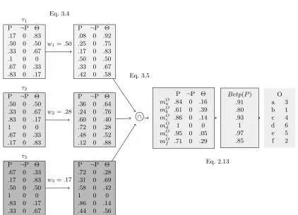
w1=.50

w2=.28

w3=.17

Figure 3.2: Example of BRE with weighting schema: weight application (Eq. 3.4), combination (Eq. 3.5) and the ranking outcome (Eq. 2.13)). The weights are computed using the mean of the rankings as true-rank estimator (Eq. 3.3).

element is described as follow:

if wj =min({w1, . . . , wN})

m′_ji(P) = mji(P) + (wj∗mji(Θ))

m′_ji(¬P) = 0

m′_ji(Θ) = 1−m′_ji(P)

if wj 6=min({w1, . . . , wN})

m′_ji(Θ) =mji(Θ) + (wj ∗mji(P))

m′_ji(¬P) = 0

m′_ji(P) = 1−m′_ji(Θ)

(3.4)

where mji is the bba of the j-th ranking on the i-th item, min(·) is the minimum

function and m′

ji is the discounted one. We apply these weights globally, namely the

(37)

3.2.4 Ranking Output

The final step of BRE is the combination of the bba of each item along all the rankings, using the conjunctive rule (Eq. 2.9) as follows:

mO_i (P) = O∩

N

j=1mji(P)

mOi (¬P) = O∩

N

j=1mji(¬P)

mOi (Θ) =O∩

N

j=1mji(Θ)

(3.5)

with i ∈ 1, . . . , n and where mO

i is the combined bba for the i-th item. The use of the

conjunctive rule is justified when all the sources of belief are assumed to tell the truth and to be independent. These requirements are fully satisfied here, since we suppose that the rankings are independent and totally reliable because the unsupervised context does not allow to make other assumptions on their quality. We apply the Eq. 2.13 on the mO

i in

order to take decisions in the frame Θ. The final rankingO = (O(1), . . . , O(i), . . . , O(n)) is produced by sorting all the items with respect to BetPi(P), that corresponds to the

probability of thei-th item of being in the right position. The combination step is done in the Combination routine in both NW version (Alg. 2) and the iterative version (Alg. 1).

3.2.5 BRE Versions

As described before, the three parts described above are embedded inside an iterative procedure that aims to replace the worst rankiing with combined ranking produced dur-ing each step as showed in the Alg. 1. The idea underlydur-ing this iterative replacement is that the ranking computed in each iteration will be more informative instead of the input rankings in terms of approximation quality of the true ranking. For the replacing of a possible good true-rank estimator, we expect that BRE will increase the quality of the true-rank estimator. The effect of the iterative procedure in the algorithm will be evaluated in details in the experimental parts (Sec. 3.4-3.5). Although there is no the-oretical constraint about the number of iterations, we propose as number of iteration

MAXT = N₂. The rational of this rule of the thumb is that replacing more then one half of the original rankings can possibly lead to poor performance due to the replacement of some of the best rankings with information affected by the worse ones.

We present three versions of BRE, one not-weighted (BRE-NW) where the rank-ings quality is not involved in the combination, the iterative version where weights and the ranking replacement are introduced and a T = 1 version without replacement.

BRE−NW, showed in Alg. 2, combines the belief distribution of the input rankings without the application of the weights. A numerical example of the BRE-NW is showed in Fig. 3.1. In the remaining of the chapter we refer as weighting schema to theBRE−1T

version, whereas as iterative schema whenT =MAXT.

(38)

truthfulness of the experts concerns the global reliability of the rankings, it is also related to the quality of the rankings with respect to the true ranking. If this information is available a priori can be directly used in BRE as input weights.

Another issue related to the a priori information available, is the possibility to known the information about each ranked item or for a subset of items. An example can be an expert that have a bias on the ranking of a subset of elements so it assigns systematically higher or lower rank values to these items in the ranking produced. Starting from this knowledge, other belief assignments should be considered, in order to map this bias into the frame Θ. A more complete scenario is when the information of the items are known

a priori for all the rankings, this can be perfectly managed into the BRE algorithm sup-ported by the Belief Function that permits to model the subjective point of view for the item of each ranking involved. The last consideration opens also the possibility to use and compute the weights for each item instead of a global weights applied to all the items of a ranking.

(39)

3.3. BRE vs. the Ranking Aggregation Methods

3.3

BRE vs. the Ranking Aggregation Methods

With respect to the classification in heuristic methods and optimization solutions for the rankings aggregation problem we can consider BRE to be an heuristic solution, since in its formulation there is no criterion to minimize. Among the state-of-the-art methods presented in Chapter 2, in the next experiments we have compared the performance of BRE with respect to the following methods: the mean and the median of the rankings (Borda Count’s method) and the Footrule optimal aggregator. We point out that BRE uses the Spearman footrule distance for the computation of the weights, so to provide a fair comparison we focus on solutions that minimize that distance. As heuristic com-petitors we use the Borda Count methods with the median and the mean as aggregation functions, where the score of each item corresponds to its rank value (BJ₍_i_{) =} _τj₍_i_)).

We simply refer to Borda Count’s methods as the mean and the median of the rankings. As for the optimal aggregator method, we include as competitor the Footrule optimal aggregator. The Footrule optimal aggregator minimizes the footrule distance with the input rankings, and it can be computed in polynomial time solving the minimum cost of matching on a weighted bipartite graph [4].

We have not included the MEDrank algorithm as competitor since we have just evalu-ated similar heuristics as the median of the rankings. Moreover the MEDrank algorithm provides the Footrule optimal aggregator in case of total rankings [17], and we have just included a similar solution as competitor.

The Markov chain methods take into account in their solutions the pairwise comparison of all the items on the rankings. We notice that the Markov chain solutions consider the problem from the point of view of the items present in the rankings. On the other hand, BRE faces the problem from the the point of the input rankings in fact the informations related to the pairwise comparison of all the items are not used. For the highlighted differences of the two approaches, we have not included the Markov chain methods as competitors.

The stochastic optimization solutions are not included as competitors on total rankings, since the Footrule optimal aggregator on total rankings is solved with acceptable compu-tational time. In general, BRE is not compared with the rankings aggregation methods based on probabilistic models since they include a step (both unsupervised and supervised solutions) where the probabilistic model learns from data. Moreover BRE and the other ranking aggregation methods are totally unsupervised solutions.

3.4

Experiment 1: BRE vs The Competitor Methods

In this section we describe the results of BRE with respect to some aggregation methods proposed in the state of the art. All the versions of BRE previously presented such as BRE-NW, BRE-1T and BRE-MAXT have been evaluated in order to highlight possible differences of performance.

(40)

aggregation methods evaluated has been given in Sec. 2.3. As true-rank estimator inside BRE we use the same ranking-aggregation competitor methods, in order to investigate if BRE increases the performance with respect to the methods used as true-rank estimator. We have not found real data on total rankings with an available true ranking. To the best of our knownledge, there is not any. For this reason we have decided to evaluate BRE on synthetic data that suits perfectly the problem at hand.

The data has been generated as follows. We have fixed a true ranking (τTrank) from

which the input rankings has been randomly generated according to fixed values of the Spearman coefficient, indicated asρ[20][22] (Eq. 2.4). The generated rankings are overall random permutations with respect to all the items contained in the true ranking. The variables that would be investigated in our experimental settings on synthetic data are the following:

– Correlation ρof the input rankings with respect to true ranking. – Number of experts (denoted as N).

Despite the space of the parameters is quite huge to be totally evaluated, we have decide to fix the length of the rankings (n= 300) in order to focus our attention on the correlation of the rankings (a measure of quality) and on the number of experts aggregated. Among all theN values we have generated a total of 10 different cases that permit to have a large picture of the BRE performance in heterogeneous situations of correlation with respect to the true ranking. The length of the rankingnhas been fixed equal to 300 for all the cases. We have evaluated a number of experts N equal to 3, 10,30. For each N value different cases of the input rankings has been proposed. For N=3 we have defined 4 cases:

Case 1 1 ranker extremely good (ρ=.80) with respect to the others (ρ=.06 ρ=.01). Case 2 two good rankers (ρ=.60, .40) and a very poor one (ρ=.01).

Case 3 3 rankers with high correlation (ρ=.80, .60, .10). Case 4 3 rankers with poor correlation (ρ=.01, .06, .03). For N = 10, 30 we have defined 3 cases each:

Case Good the 80% of the rankers are highly informative (ρ ∈ [.95, .70]) and the re-maining 20% are low correlated (ρ∈[.30, .10]).

Case Equal The rankers are equally distributed among the three types: highly, medium

(ρ∈[.70, .30]) and low correlated.

Case Poor The opposite of the case good, 80% of the rankers are poorly informative and only the 20% are hightly correlated.

(41)

3.4. Experiment 1: BRE vs The Competitor Methods

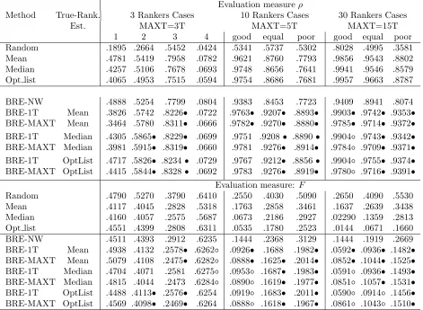
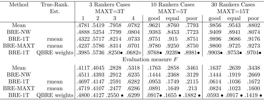
Table 3.1: Spearman correlation coefficent (ρ) and Spearman Footrule distance (F) of BRE and of the competitor methods with respect to the true ranking. means that BRE is significantly better than

the corresponding competitor, and means that BRE is significantly worse.

Evaluation measureρ

Method True-Rank. 3 Rankers Cases 10 Rankers Cases 30 Rankers Cases

Est. MAXT=3T MAXT=5T MAXT=15T

1 2 3 4 good equal poor good equal poor Random .1895 .2664 .5452 .0424 .5341 .5737 .5302 .8028 .4995 .3581 Mean .4781 .5419 .7958 .0782 .9621 .8760 .7793 .9856 .9543 .8802 Median .4257 .5106 .7678 .0693 .9748 .8656 .7641 .9941 .9546 .8579 Opt list .4065 .4953 .7515 .0594 .9754 .8686 .7681 .9957 .9663 .8787

BRE-NW .4888 .5254 .7799 .0804 .9383 .8453 .7723 .9409 .8941 .8074 BRE-1T Mean .3826 .5742 .8226 .0722 .9763 .9207 .8893 .9903 .9742 .9353

BRE-MAXT Mean .3464 .5780 .8311 .0666 .9782 .9270 .8880 .9785 .9714 .9372

BRE-1T Median .4305 .5865 .8229 .0699 .9751 .9208 .8890 .9904 .9743 .9342

BRE-MAXT Median .3981 .5915 .8319 .0660 .9781 .9276 .8914 .9784 .9709 .9371

BRE-1T OptList .4717 .5826 .8234 .0729 .9767 .9212 .8856 .9904 .9755 .9374

BRE-MAXT OptList .4415 .5844 .8328 .0692 .9783 .9276 .8919 .9780 .9716 .9391

Evaluation measure: F

Random .4790 .5270 .3790 .6410 .2550 .4030 .5090 .2650 .4090 .5530 Mean .4117 .4045 .2828 .5318 .1763 .2858 .3461 .1637 .2639 .3438 Median .4160 .4057 .2575 .5687 .0673 .2186 .2927 .02290 .1359 .2813 Opt list .4551 .4399 .2808 .6311 .0535 .1780 .2523 .0144 .0671 .1660 BRE-NW .4511 .4393 .2912 .6235 .1444 .2368 .3129 .1444 .1919 .2669 BRE-1T Mean .4938 .4132 .2578 .6262 .0926 .1688 .1982 .0592 .0936 .1482

BRE-MAXT Mean .5079 .4108 .2475 .6282 .0888 .1625 .2014 .0852 .1044 .1525

BRE-1T Median .4704 .4071 .2581 .6275 .0953 .1687 .1983 .0591 .0936 .1493

BRE-MAXT Median .4815 .4044 .2473 .6284 .0890 .1619 .1977 .0851 .1057 .1531

BRE-1T OptList .4488 .4113 .2576 .6254 .0919 .1683 .2011 .0590 .0914 .1456

BRE-MAXT OptList .4569 .4098 .2469 .6264 .0888 .1618 .1967 .0861 .1043 .1510

performance is measured with the Spearman correlation coefficient (ρ, Eq. 2.4) and the Spearman Footrule distance (F) computed with respect to the true ranking (τTrank).

In Tab. 3.1, we show the significance of the results of BRE with respect to the true-ranking estimator method used. In the discussion the significance has been also evaluated such as BRE-1T vs. BRE-MAXT and BRE-1T vs. BRE-NW.

In Tab. 3.1, we also present a competitor calledrandom, that corresponds to a ranking chosen uniformely randomly among the input rankings. Since BRE-1T is significantly better than the random competitor in all the cases and for both the evaluation measures, we can assert that the BRE results are very far from a random guess.

(42)

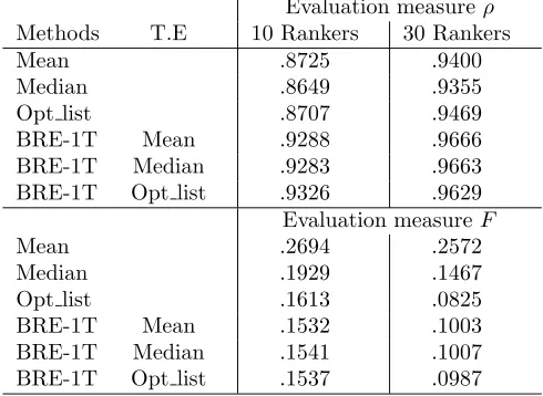
Table 3.2: Average Spearman correlation coefficent (ρ) and Spearman Footrule distance (F) of BRE and of the other competitors with respect to true ranking for thegood, equal and poor cases withN = 10,30

Evaluation measureρ

Methods T.E 10 Rankers 30 Rankers

Mean .8725 .9400

Median .8649 .9355

Opt list .8707 .9469

BRE-1T Mean .9288 .9666

BRE-1T Median .9283 .9663 BRE-1T Opt list .9326 .9629 Evaluation measureF

Mean .2694 .2572

Median .1929 .1467

Opt list .1613 .0825

BRE-1T Mean .1532 .1003

BRE-1T Median .1541 .1007 BRE-1T Opt list .1537 .0987

highlights a significant improvement with respect to the mean in terms ofF andρ, whereas the mean is influenced by the low-quality rankings.

Taking into account the median as the true-rank estimator, we notice that BRE-1T outperforms the median as competitor method in most of the evaluated cases for both evaluation measures, except for the case good withN =30 where the median outperforms our BRE. Also for the median, BRE-1T performance shows a significant improvement in the cases poor for N = 10, 30 with both the evaluation measures.

Opt list shows the best values of ρ and F with respect to the mean and the median in all the three cases with N = 30 and N = 10. BRE-1T with Opt list as estimator outperforms significantly the Opt list method in all cases poor (N = 10, 30) , except for the case good (N = 30, 10) and the case equal with N = 10 where Opt List shows the best results among all the other ranking aggregation competitors with F distance. From Tab. 3.1, we notice that BRE-MAXT shows significant improvement with respect to the estimators in same cases against the 1T version. From the comparison of BRE-1T with respect to BRE-MAXT, we point out that in the cases good and equal (N = 10), BRE-MAXT outperforms significantly the 1T version even if for small differences of ρ

and F. On the other hand, increasing the number of rankings (N = 30) the BRE-MAXT looses its positive edge. This flaw of the BRE-MAXT performance can be explained due to the fact that a lot of quite similar rankings are included into the combination by the replacing process.

(43)

3.4. Experiment 1: BRE vs The Competitor Methods

We point out that in a real situation the quality of the input rankings or their distribu-tion is unknown. It can be quite difficult to determine if the rankings are heterogeneous or homogeneous in terms of quality with respect to the true ranking. This may introduce doubts about whether to apply BRE or other aggregation methods. Taking into account the average results amo