pa o l o p i vat o
A N A LY S I S A N D C H A R A C T E R I Z AT I O N O F W I R E L E S S P O S I T I O N I N G T E C H N I Q U E S I N I N D O O R E N V I R O N M E N T
International Doctoral School in Information and Communication Technology XXV Cycle
Department of Information Engineering and Computer Science
University of Trento
Doctoral Dissertation of:
pa o l o p i vat o
Advisor:
p r o f. d a r i o p e t r i
Co-Advisor:
p r o f. l u i g i pa l o p o l i
e x a m i nat i o n c o m m i t t e e:
prof.d a r i o p e t r i Chair, Advisor prof.l u i g i pa l o p o l i Co-Advisor prof.c l au d i o na r d u z z i Member prof.a n t o n i o m o s c h i t ta Member
P U B L I C AT I O N S
i n t e r nat i o na l j o u r na l s
[J1] P. Pivato, L. Palopoli, and D. Petri, “Accuracy of RSS-Based Cen-troid Localization Algorithms in an Indoor Environment,”IEEE Transactions on Instrumentation and Measurement, vol. 60, no. 10, pp. 3451–3460, Oct. 2011.
[J2] D. Macii, A. Colombo, P. Pivato, and D. Fontanelli, “A Data Fu-sion Technique for Wireless Ranging Performance Improvement,” IEEE Transactions on Instrumentation and Measurement, vol. 61, no. 1, pp. 27–37, Jan. 2013.
i n t e r nat i o na l c o n f e r e n c e s
[C1] P. Pivato, S. Dalpez, and D. Macii, “Performance Evaluation of Chirp Spread Spectrum Ranging for Indoor Embedded Naviga-tion Systems,” in Proc. 7th IEEE International Symposium on In-dustrial Embedded Systems (SIES 2012), Karlsruhe, Germany, Jun. 2012, pp. 1–4.
[C2] C. M. De Dominicis, P. Ferrari, E. Sisinni, A. Flammini, P. Pivato, and D. Macii, “Timestamping Performance Analysis of IEEE 802.15.4a Systems based on SDR Platforms,” in Proc. IEEE In-ternational Instrumentation and Measurement Technology Conference (I2MTC 2012), Graz, Austria, May 2012, pp. 2034–2039.
[C3] P. Pivato, S. Dalpez, D. Macii, and D. Petri, “A Wearable Wireless Sensor Node for Body Fall Detection,” inProc. IEEE International Workshop on Measurement and Networking (M&N 2011), Anacapri, Italy, Oct. 2011, pp. 116–121.
[C4] D. Macii, P. Pivato, and F. Trenti, “A Robust Wireless Proximity Detection Techniques based on RSS and ToF measurements,” in Proc. IEEE International Workshop on Measurement and Networking (M&N 2011), Anacapri, Italy, Oct. 2011, pp. 31–36.
[C5] P. Pivato, L. Fontana, L. Palopoli, and D. Petri, “Experimental Assessment of a RSS-based Localization Algorithm in Indoor En-vironment,” in Proc. IEEE International Instrumentation and
surement Technology Conference (I2MTC 2010), Austin, TX, USA, May 2010, pp. 416–421.
[C6] M. Corra, L. Zuech, C. Torghele, P. Pivato, D. Macii, and D. Petri, “WSNAP: a Flexible Platform for Wireless Sensor Networks Data Collection and Management,” in Proc. IEEE Workshop on Environmental, Energy, and Structural Monitoring Systems (EESMS 2009), Crema, Italy, Sep. 2009, pp. 1–7.
A C K N O W L E D G M E N T S
I would like to thank my advisor, prof. Dario Petri, and my co-advisor, prof. Luigi Palopoli, for their valuable guidance and support during my Ph.D., teaching me the values of objectivity and independence in doing research.
A dutiful thank you to prof. David Macii for his professionalism and humanity shown to me several times.
C O N T E N T S
1 i n t r o d u c t i o n 1
1.1 Objectives and Novel Contribution of the Research . . 2
1.2 Thesis Organization . . . 3
2 s tat e o f t h e a r t 5 2.1 Introduction . . . 5
2.2 Positioning Techniques . . . 6
2.2.1 Lateration . . . 6
2.2.2 Angulation . . . 7
2.3 Wireless Ranging . . . 8
2.3.1 Received-Signal-Strength Ranging . . . 9
2.3.2 Time-of-Flight Ranging . . . 11
2.4 Related Work . . . 13
2.4.1 Infrared . . . 13
2.4.2 Ultrasound . . . 14
2.4.3 Radio-frequency . . . 14
3 r s s-b a s e d r a n g i n g a n d p o s i t i o n i n g i n i n d o o r e n -v i r o n m e n t 17 3.1 Introduction . . . 17
3.2 Measurement Context . . . 19
3.3 RF Channel Characterization . . . 20
3.3.1 Indoor RF Channel Propagation Model . . . 20
3.3.2 RF Channel Parameters Estimation . . . 23
3.4 Localization Algorithms . . . 26
3.4.1 Weighted Centroid Localization . . . 26
3.4.2 Relative Span Exponential Weighted Localization 30 3.5 Conclusion . . . 36
4 h y b r i d r s s-r t t m e t h o d f o r r a n g i n g p e r f o r m a n c e i m p r ov e m e n t 39 4.1 Introduction . . . 39
4.2 Uncertainty of RSS and RTT Ranging Techniques . . . 40
4.3 Data Fusion Algorithm for Distance Estimation . . . . 43
4.3.1 Data Acquisition and Filtering . . . 44
4.3.2 System Model . . . 47
x c o n t e n t s
4.3.3 Kalman Filter Definition . . . 48
4.3.4 Data Fusion . . . 49
4.4 Hardware Platform Description . . . 49
4.5 Experimental Results . . . 52
4.5.1 Uncertainty Evaluation of Individual Quantities 52 4.5.2 Accuracy Analysis in Dynamic Conditions . . . 56
4.6 Conclusion . . . 60
5 t i m e s ta m p i n g o f i e e e 802.15.4a c s s s i g na l s 63 5.1 Introduction . . . 63
5.2 Overview of IEEE 802.15.4a Chirp Spread Spectrum . . 66
5.3 Theoretical Model . . . 70
5.4 Uncertainty Analysis and Symbol Timestamp Definition 72 5.4.1 Incoherent baseband sampling and finite tem-poral resolution . . . 73
5.4.2 Wideband Noise . . . 74
5.4.3 Frequency Offsets . . . 74
5.4.4 Multipath Propagation . . . 78
5.4.5 Definition of Symbol Timestamp . . . 80
5.5 Experimental Characterization . . . 81
5.5.1 Experimental Setup . . . 81
5.5.2 Performance Metrics . . . 83
5.6 Experimental Results . . . 84
5.7 Conclusion . . . 86
6 c o n c l u s i o n 89 6.1 Contributions . . . 91
6.2 Future Research Work . . . 92
a e q u i va l e n c e b e t w e e n r e w l a n d w c l a l g o r i t h m s 93
L I S T O F F I G U R E S
Figure 2.1 Lateration positioning method. . . 7
Figure 2.2 Angulation positioning method. . . 8
Figure 3.1 Location test points within the Domotic Appli-cation Lab. . . 18
Figure 3.2 RSS measurements and related channel models 22
Figure 3.3 RSS error histograms . . . 25
Figure 3.4 WCL distance error . . . 29
Figure 3.5 WCL algorithm errors cumulative histograms 33
Figure 3.6 REWL distance error . . . 35
Figure 3.7 REWL algorithm errors cumulative histograms 37
Figure 4.1 Distance estimation algorithm block diagram . 45
Figure 4.2 Functional block diagram and snapshot of the Mobile Tracking System . . . 50
Figure 4.3 RSS- and ToF-based distance measurements stan-dard uncertainty and RMSE values . . . 54
Figure 4.4 Average probability of using the heuristic cri-terion as a function of the MA window size . . 55
Figure 4.5 Average RMSE patterns related to different RSS-and ToF-based distance estimators . . . 55
Figure 4.6 Histogram of the measured sampling time val-ues. . . 57
Figure 4.7 Measurement results obtained with the pro-posed data fusion algorithm . . . 59
Figure 4.8 Distance uncertainty box-and-whiskers plot: tar-get moving along a straight line . . . 61
Figure 4.9 Distance uncertainty box-and-whiskers plot: tar-get moving along an arc of circle . . . 61
Figure 5.1 Qualitative shape of four different IEEE 802.15.4a CSS symbols as a function of time . . . 67
Figure 5.2 IEEE 802.15.4a subchirp correlation pulse for
k=2 . . . 72
Figure 5.3 Effect of AWGN on timestamping jitter . . . . 75
Figure 5.4 Mean value and standard deviation of εo as a function of different systematic transmitter-receiver frequency offsets for subchirpsk=2 . 77
Figure 5.5 Distribution of εp in the presence of a strong multipath interference for a mean interarrival
time equal to5ns . . . 79
Figure 5.6 Definition and benefits of IEEE 802.15.4a CSS frame timestamping at the symbol level. . . 81
Figure 5.7 Symbol timestamping on the timescales of trans-mitter and receiver . . . 82
Figure 5.8 Distribution of the symbol timestamping er-rors in the case of data transfers between two N210 platforms . . . 87
L I S T O F TA B L E S Table 2.1 Comparison of indoor positioning systems . . 14
Table 3.1 Log-normal channel parameters . . . 24
Table 3.2 WCL algorithm mean distance error . . . 31
Table 3.3 WCL algorithm RMS distance error . . . 31
Table 3.4 REWL algorithm mean distance error . . . 34
Table 3.5 REWL algorithm RMS distance error . . . 34
Table 5.1 Sub-band center frequencies, chirping directions and temporal parameter of subchirps . . . 69
Table 5.2 Post-interpolation errors for 10 different frac-tional delays between0andTs. . . 73
Table 5.3 Single subchirp timestamping accuracy analysis. 84 Table 5.4 Symbol timestamping accuracy analysis. . . . 85
A C R O N Y M S A N D A B B R E V I AT I O N S
2D two-dimensional 3D three-dimensional AAL ambient assisted living ACK acknowledgement
a c r o n y m s a n d a b b r e v i at i o n s xiii
ADC analog-to-digital converter AoA angle-of-arrival
ATS Average TimeSynch
AWGN additive white Gaussian noise BS base station
CL centroid localization COTS commercial off-the-shelf CRB Crámer-Rao bound
CSMA carrier sense multiple access
CSMA-CA carrier sense multiple access with collision avoidance CSS chirp spread spectrum
DAC digital-to-analog converter DCR direct conversion receiver DDC digital down-converter
DQPSK differential quadrature phase-shift keying DUC digital up-converter
ENBW equivalent noise bandwidth FA fixed anchor
FIR finite impulse response
FPGA field programmable gate array
FTSP Flooding Time Synchronization Protocol GNSS global navigation satellite system
GPS global positioning system ID identification data
IEEE Institute of Electrical and Electronic Engineers IIR infinite impulse response
xiv a c r o n y m s a n d a b b r e v i at i o n s
ISI intersymbol interference KF Kalman filter
KF A Kalman filter A KF B Kalman filter B LOS line-of-sight
LR-WPAN low-rate wireless personal area network LSM least squares method
MA moving-average MAC media access control MCU microcontroller unit MT mobile target
MTS mobile tracking system NLOS non-line-of-sight OWR one-way ranging PAN personal area network PDA personal device assistant PHY physical layer
PTP Precision Time Protocol RAM random-access memory
RBS Reference-Broadcast Synchronization
REWL relative-span exponential weighted localization RF radio-frequency
RFID radio-frequency identification RMS root-mean square
RMSE root-mean-square error RSS received-signal-strength
a c r o n y m s a n d a b b r e v i at i o n s xv
RTT round-trip time RX receiver
SD secure digital
SDR software-defined radio SFD start frame delimiter SNR signal-to-noise ratio SPI serial peripheral interface TDC time-to-digital converter TDoA time-difference-of-arrival ToA time-of-arrival
ToF time-of-flight
TDMA time-division multiple access TWR two-way ranging
TX transmitter
USB universal serial bus
USRP universal software radio peripheral UWB ultra-wide band
1
I N T R O D U C T I O N
I
ndoor positioning, also referred to as indoor localization, shall be defined as the process of providing accurate people or objects co-ordinates inside a covered structure, such as an airport, an hospital, and any other building.The applications and services which are enabled by indoor localiza-tion are various, and their number is constantly growing. Industrial monitoring and control, home automation and safety, security, logis-tics, information services, ubiquitous computing, health care, and ambient assisted living (AAL) are just a few of the domains that in-door positioning technology can benefit. A significant example is of-fered by local information pushing. In this case, a positioning system sends information to a user based on her/his location. For instance, a processing plant may push workflow information to employees re-garding operating and safety procedures relevant to their locations in the plant. The positioning system tracks each employee, and has knowledge of the floor plan of the facility as well as the procedures. When an employee walks inside a defined perimeter of a particular area, such as packaging department, the positioning systems displays on the user’s personal device assistant (PDA) information regarding the work expected to be done in that area This significantly increases efficiency and safety by ensuring that employees follow carefully de-signed guidelines. Location-enabled applications like this are becom-ing commonplace and will play important roles in our everyday life.
The design of a positioning system for indoor applications is to be regarded as a challenging task. In fact, the global positioning sys-tem (GPS) is a great solution for outdoor uses, but its applicability is strongly limited indoors because the signals coming from GPS satel-lites cannot penetrate the structure of most buildings. For this rea-son, considerable research interest for alternative non-satellite-based indoor positioning solutions has arisen in the last years.
Actually, the positioning problem is strictly related with the mea-surement of the distance between the object to be located and a num-ber of landmarks with known coordinates. Then, the position of the
2 i n t r o d u c t i o n
target is commonly determined by means of appropriate statistical or geometrical algorithms.
Several approaches have been proposed, and various are the funda-mental technologies that have been used so far. Today, distance mea-surement between two objects can be easily obtained by using laser-, optical- and ultrasounds-based devices. However, evident drawbacks of these systems are their sensitivity to line-of-sight (LOS) constraint, and the strict object-to-object bearing requirement. The latter becomes an even worse downside when the topology of the system dynami-cally changes due to mobility of the target.
On the other hand, wireless-based ranging solutions are more in-sensitive to obstacles and non-alignment condition of devices. In ad-dition, they may take advantage of existing radio modules and in-frastructures used for communications. Accordingly, the ever grow-ing popularity of mobile and portable embedded devices provided with wireless connectivity has encouraged the study and the develop-ment of radio-frequency (RF)-based positioning techniques. The core of such systems is the measurement of distance-related parameters of the wireless signal.
The two most common approaches for wireless ranging are based on received-signal-strength (RSS) and message time-of-flight (ToF) measurements, respectively. In particular:
• the RSS-based method relies on the relationship between the measured received signal power and the transmitter-receiver distance, assuming that the signal propagation model and the transmitted power are known;
• the ToF-based technique leans on the measured signal propa-gation time and the light speed, owing to the fundamental law that relates distance to time.
1.1 o b j e c t i v e s a n d n ov e l c o n t r i b u t i o n o f t h e r e s e a r c h
The work presented in this dissertation is aimed at investigating and defining novel techniques for positioning in indoor environment based on wireless distance measurements.
1.2 t h e s i s o r g a n i z at i o n 3
for the localization of objects inside buildings. Nevertheless, several limitations exist (e.g., on the accuracy of the ranging, its impact on localization algorithms, etc.).
The work presented in this dissertation attempts to:
1. investigate the main sources of uncertainty affecting RSS- and ToF-based indoor distance measurement;
2. analyze the impact of ranging error on the accuracy of position-ing;
3. propose, on the basis of the understanding gained from 1. and 2., novel and effective systems in order to overcome the above-mentioned limitations and improve localization performance. The novel contributions of this thesis can be summarized as fol-lows:
• In-depth analysis of both RSS- and ToF-based distance measure-ment techniques, in order to assess advantages and disadvan-tages of each of them.
• Guidelines for using different ranging methods in different con-ditions and applications.
• Implementation and field testing of a novel data fusion algo-rithm combining both RSS and ToF techniques to improve rang-ing accuracy.
• Theoretical and simulation-based analysis of chirp spread spec-trum (CSS) signals for low-level timestamping.
• Experimental assessment of CSS-based timestamping as key en-abler for high accuracy ToF-based ranging and time synchro-nization.
1.2 t h e s i s o r g a n i z at i o n
This thesis is organized in six Chapters, including the present one, and one Appendix.
4 i n t r o d u c t i o n
Chapter 3 analyze the accuracy of indoor localization based on RSS measurements in a wireless sensor network (WSN). Two differ-ent classes of low-computational-effort algorithms based on the cen-troid concept are considered. The different sources of measurement uncertainty are investigated by means of theoretical simulations and experimental results.
Chapter 4examines in detail the RSS and ToF methods in order to evaluate the main uncertainty contributions affecting either measure-ment procedure. This preliminary analysis serves as the basis for the proposal of a new data fusion algorithm combining both techniques in order to improve ranging accuracy. The implementation of the pro-posed algorithm is discussed, and several experimental results are provided to prove the efficacy of the algorithm in reducing measure-ment uncertainty.
Chapter 5 introduces the main features of the CSS physical layer (PHY) described in the amendment IEEE 802.15.a-2007 and discusses the basic CSS signal detection problem in ideal conditions and under the effect of various uncertainty contributions. In particular, an opti-mal solution for frame timestamping at the symbol level is proposed. Some experimental results based on a software-defined radio (SDR) implementation of the IEEE 802.15.4a PHY show that CSS can be suc-cessfully adopted for accurate ranging and, as side effect, also for time synchronization.
2
S TAT E O F T H E A R T
2.1 i n t r o d u c t i o n
A
s alreadymentioned in the Introduction,positioning, also called localization, can be generally defined as the process of finding location coordinates of people or objects within a reference frame, in a two-dimensional (2D) or three-dimensional (3D) space.In the last years, the astonishing growth of mobile and portable devices provided with wireless connectivity has paved the way for the development of positioning systems relying on the measurement of different location-related parameters of the wireless signal. For instance, signal strength of an RF link notoriously depends on the range between transmitter and receiver, according to a law whose details depend on the propagation model of the physical environ-ment where communication occurs. Similarly, RF signal propagation time depends on the distance between the communicating devices, and can be determined by knowing the signal propagation speed in the medium. Furthermore, the angle at which RF signal arrives at the receiver yields important information about the position of the transmitter, and can be related to the transmitter-receiver separation as well. Accordingly, distance can be indirectly determined from the measurement of such parameters, and later processed by means of appropriate methods to estimate the position.
Probably, the best known and most widespread example of wire-less localization technique is the global positioning system (GPS). However, it is not the ultimate solution for all location-enabled ap-plications. In fact, GPS fulfills the demand for outdoor localization, where the devices can receive the signals coming from satellites, but its performance drastically deteriorates in the presence of obstruc-tions limiting the LOS, e.g., inside of buildings. The fact that indoor environments cannot take advantage of GPS has fostered the research for alternative non-satellite-based positioning solutions.
Within this context, we speak of wireless indoor positioning when the location procedure is performed using wireless systems and the reference frame is placed in indoor environment. One more
6 s tat e o f t h e a r t
tion is needed. Broadly speaking, especially in the literature, various positioning systems are referred to aswirelessin the sense that they re-quireno electric wiring. In this work, the termwirelessrefers exclusively to systems based onRF technologiesthat rely on distance estimates to determine the location of an object.
In the remainder of this Chapter, we aim to provide an overview of wireless indoor positioning systems, as a means of establishing a background for the present research. First, we describe the methods used to derive the location of an object through position-related mea-surements of the wireless link. Then, we focus on the range-based po-sitioning approach and, in particular, on the techniques used to infer distance estimates from RF signal measurements. Finally, we review the relevant literature on the subject.
2.2 p o s i t i o n i n g t e c h n i q u e s
Before we delve deep into the depths of wireless indoor positioning techniques, it is useful to introduce a generalized scenario that, re-gardless of the underlying technology and the final application, may describe the fundamental tasks that a positioning system is expected to perform. Within this generalized scenario, the essential require-ment is the communication between a device that need to be localized and a set of reference devices with fixed specific coordinates. Accord-ing to the context of the scenario beAccord-ing discussed and in agreement with terms commonly used in the literature, along this thesis we in-terchangeably use the words target, object, mobile, and combinations of thereof to indicate the wireless device whose location coordinates have to be estimated. Similarly, any reference device with known po-sition coordinates used to accomplish the location process is usually referred to asanchor,beacon,reference, orlandmark. In both cases, above mentioned terms are often followed by the wordnodeordevice.
2.2.1 Lateration
2.2 p o s i t i o n i n g t e c h n i q u e s 7
A B
C
P
P00 P000
P0
ρA
ρB ρC
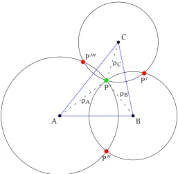
Figure 2.1: Lateration positioning method.
The most commonly used positioning technique determines target location by finding the intersection of circles with centers correspond-ing to the anchors coordinates and radii the distances from the target [1]. This range-based method is usually calledmultilateration. In ideal conditions, i.e., in the absence of noise or ranging errors, three in-tersecting circles, i.e., three anchors, are sufficient to achieve target location without ambiguity in a 2D space. In this case, the process is referred to as trilateration, since the anchors layout represents a triangle. Figure 2.1shows an example. A, Band C denote three an-chors whose coordinates in a reference system are known, whereas
P denotes a target whose position has to be determined. All the four devices lie in the same plane. The intersection of the circles centered in A,B, andC, with radiiρA, ρB, andρC, respectively, is marked in green and represents the location of targetP. The intersectionsP0,P00, andP000, respectively, are marked in red and point out the ambiguities that would be caused if only two anchors were used.
2.2.2 Angulation
8 s tat e o f t h e a r t
Figure 2.2: Angulation positioning method.
method is traditionally known as angulation. In the case of no noise or angle measurement inaccuracies, at least two target-to-anchor bear-ing lines are required to obtain positionbear-ing in a 2D space [1], as shown in Figure 2.2. LetAandBdenote two anchors whose coordinates in a reference system are known, andP denote a target whose position has to be determined. The three devices are in the same plane. The intersection of the bearing lines through A andB, with slopeα and
β, respectively, indicates the location of targetP. The coordinates ofP
can be computed by measuring angles αand βand considering the distance betweenAandBfound from their known coordinates.
2.3 w i r e l e s s r a n g i n g
Certainly, distance measurement forms the heart of any range-based positioning system. As a consequence, the accuracy of positioning strongly depends on the accuracy of ranging.
ac-2.3 w i r e l e s s r a n g i n g 9
curacy in the short range is notoriously quite hard and, consequently, it is still a hot research topic worldwide.
Camera-based solutions are very effective in terms of accuracy, even in the presence of partial occlusions. However, they are not always us-able because of privacy issues and because they suffer from scalabil-ity problems. To overcome the directional constraint of such systems, pan-tilt and omni-directional cameras have been also proposed [8]. Their main drawback is the high computational burden when multi-ple targets have to be recognized and tracked.
The most accurate approach is provided by laser-based systems, e.g., based on scanning heads, which also address the target pointing problem [9]. Unfortunately, these systems are much more expensive than the other solutions.
RF-based ranging techniques are inherently less sensitive to obsta-cles and dissipate less power than optical and ultrasound solutions. In addition, they may exploit the same wireless modules used for communication and they are particularly suitable for wearable in-door applications. As stated before, in wireless distance measurement techniques the range between two objects is obtained indirectly from some distance-related parameters of the RF signal. The two most com-mon approaches are based on RSS and signal ToF measurements. In the following Sections we present the fundamental aspects of RSS and ToF techniques, discussing the different phenomena that limit the accuracy of these measurements.
2.3.1 Received-Signal-Strength Ranging
The RSS-based ranging technique relies on the relationship between the measured received signal power and the transmitter-receiver dis-tance. If the transmitted power and the signal propagation model are known, the distance from the transmitter can be estimated by revers-ing the equation of the model.
The fundamental propagation model predicting the received signal-strength at a given distance from the transmitter in LOS path condi-tions is the so-calledfree-spacepath loss model [10]. It is described by the well-known free-space Friis equation as
s=stgtgt
λ 4πd
2
10 s tat e o f t h e a r t
where s is the received signal power, st is the transmitted signal power, gt and gr are transmitter and receiver antenna gains respec-tively, dis the distance between transmitter and receiver (expressed in meters) and λ is the wavelength (expressed in meters). Clearly, (2.1) does not hold when d equals to zero. Moreover, the Friis free-space model is valid only for values ofdwhich are in the far-field, or Fraunhofer region, of the transmitting antenna. For this reason, a ref-erence distance denoted asd0is introduced in the model as a known received power reference point in free-space. The value of such ref-erence distance must be chosen so that it lies in the far-field region of the transmitting antenna and is smaller than any other distance considered in the wireless link. Then, the received power s at any distancedfrom the transmitter greater thand0 can be expressed as
s=s0
d0 d
2
(2.2)
wheres0is the received power atd0, which can be derived from (2.1), or by considering the average received power at several points located at a radial distance d0 from the transmitter. When the transmitted powerst or the received powers0 at the reference point is known, it is easy to obtain the range between transmitter and receiver in free-space LOS conditions by reversing (2.1) or (2.2), respectively.
However, in practical wireless link the propagation path between transmitter and receiver may be non-line-of-sight (NLOS). Moreover, signal propagation can be subjected to the effect of various propaga-tion phenomena such as reflecpropaga-tion, diffracpropaga-tion and scattering, which alter the relationship between received power and distance. A num-ber of propagation models which take into account the different fac-tors impacting on signal propagation have been proposed in the lit-erature, both for indoor and outdoor environments. Among these, a model widely adopted in indoor environments is thelog-distance shad-owing path loss model [10]. It can be considered as a generalization of the free-space path loss model and is given by
s(t) =s0−10log
d d0
η
+w (2.3)
where s(t) is a random variable describing the received power (ex-pressed in decibels) at time t and distance d from the transmitter, s0 is the random variable modeling the received power (expressed
2.3 w i r e l e s s r a n g i n g 11
i.e., the rate at which the signal power decays with respect to distance, andwis a random variable with zero mean and varianceσ2
w, which
accounts for the random shadowing effects occurring over a large number of measurement positions which have the same distance be-tween transmitter and receiver, but have different levels of clutter on the propagation path. From (2.3) the distance between transmitter and receiver can be readily estimated as follows
dR(t) =d0·10
s0−s(t)
10·η (2.4)
Usually the RSS can be measured easily and without additional cir-cuitry, because most of integrated wireless chips are natively equipped with a received-signal-strength indicator (RSSI). In recent years, the RSS-based ranging has been widely analyzed both theoretically and experimentally. An exhaustive empirical analysis of this method is available in [11, 12]. The main drawback of RSS-based distance mea-surements is its considerable sensitivity to multipath and shadowing phenomena, which are particularly critical indoor for IEEE 802.15.4 networks [13, 14]. Some researchers state that the performance of RSS-based approaches cannot be significantly improved by means of signal processing techniques, since it is limited by the intrinsic vari-ability of the RSS in the chosen environment [15]. However, other authors believe that the total uncertainty can be mitigated through subsequent refinements [16].
2.3.2 Time-of-Flight Ranging
The ToF-based ranging method relies on the measurement of the propagation time of the RF signal. In general, two alternative ToF-based distance measurement techniques exist, i.e., the time-of-arrival (ToA) and the round-trip time (RTT) approach, respectively.
The ToA technique, also known as one-way ranging (OWR), relies on the estimation of the propagation time of a signal traveling be-tween two wireless devices [17]. In particular, the estimated distance results from the product of the signal propagation time and the light speed. However, the OWR technique requires that the transmitter and the receiver are tightly synchronized (i.e. in the order of1ns or less for short-range communications), which is particularly challenging [18].
be-12 s tat e o f t h e a r t
tween the time instant when a message is sent and the time instant when the corresponding response message is received by the same device [19]. In this case, the ToF value is obtained by dividing the measured RTT by two after removing the time spent by the message on either devices [20, 21]. Since the RTT is measured by the same node, no clock synchronization is required. For this reason, this ap-proach is more frequently used. In principle, using the RTT method the distance between transmitter and receiver can be easily estimated as follows
dT(t) = c 2·
τ(t) −oτ(t)
(2.5) whereτ(t)is a random variable modeling the total RTT,cis the speed of light, andoτ(t)is the random temporal overhead given by the sum
of:
• the latency between the moment when a message is timestam-ped on the sender side and the moment when the correspond-ing bit actually leaves the antenna;
• the time spent on the destination node to receive the incoming message and to reply with an acknowledgement (ACK) mes-sage;
• the latency between the moment when the first bit of the ACK message reaches the antenna and the moment when the mes-sage is timestamped by the receiver.
2.4 r e l at e d w o r k 13
technologies (e.g., based on the standard IEEE 802.15.4), accuracy typ-ically drops due to the large random jitter associated with time inter-val measurements [26].
2.4 r e l at e d w o r k
A number of indoor positioning systems have been developed in the last years to meet distinctive requirements of various applications and services.
Considering recent advances in this emerging field, performance evaluations of systems created almost ten years ago are hardly valid today to represent a useful state-of-the-art background. Moreover, most updated surveys on indoor positioning systems available in the literature highlight variety in the applications addressed, conceptual heterogeneity, and differences in design and in the adopted technol-ogy [27, 28]. Therefore, it is difficult – if not impossible – to accom-plish objective performance comparison and benchmarking between several systems. Furthermore, it is beyond the scope of our research to provide a complete overview of positioning systems available till now. Nevertheless, we think it is worthwhile reviewing the most sig-nificant work in the field of indoor positioning systems, despite of their age or the outdated technique used, reviewing the key features of each of them.
A number of classification schemes are used in the literature to sur-vey indoor positioning systems. In this dissertation, we classify the systems based on their enabling technology. Table 2.1 summarizes the main features of indoor positioning solutions reviewed in the fol-lowing Sections.
2.4.1 Infrared
14 s tat e o f t h e a r t
Table 2.1: Comparison of various indoor positioning systems.
s y s t e m t e c h n o l o g y m e t h o d o l o g y a c c u r a c y
Active Badge (1992) Infrared Proximity Room level
Active Bat (1997) Ultrasounds ToF, lateration 3cm
SpotON (2000) RFID RSS, lateration 3m
RADAR (2000) WLAN RSS, fingerprinting 3m
Ubisense (2005) UWB TDoA, AoA, triangulation 15cm
is located. Although infrared technology is inexpensive, the system has a number of drawbacks due to the characteristics of infrared sig-nals, i.e., short range (about4m), reflections, sensitivity to fluorescent lighting and direct sunlight.
2.4.2 Ultrasound
Active Bat [30] is widely regarded as the pioneering system for indoor people localization based on ultrasound technology. Similarly to the Active Badge system, whose represents an evolution, the Ac-tive Bat platform consists of an ultrasonic transmitter worn by each person to be located – the so-called Bat – and several ultrasonic re-ceivers mounted on the ceiling. The transmitter periodically sends a short pulse of ultrasounds that are received by a network of re-ceivers mounted on the ceiling in fixed known positions. The loca-tion of the user carrying the Bat is determined through lateraloca-tion by means of ToF-based distance measurements. In addition, the system implements a statistical rejection algorithm in order to eliminate large ranging errors due to reflections of the ultrasonic signals. An exper-imental test bed consisting of 720receivers deployed over a1000m2 ceiling and 75 transceivers provided a localization accuracy of 3cm for95% of the measurements. However, the large number of receivers needed to achieve high accuracy is very demanding both in terms of cost and deployment time, thus limiting the scalability of the system.
2.4.3 Radio-frequency
2.4 r e l at e d w o r k 15
the lateration method on inter-tag distances derived from RSS mea-surements of the signal. The system has significant limitations due to the poor location accuracy, of about 3m, and the long time required to accomplish the positioning process, i.e., between10 and20s.
RADAR [32] provides one of the first experimental works on in-door positioning based on IEEE 802.11 wireless local area network (WLAN) technology. The system adopts the RSS mapping technique, i.e., a database of RSS-location pairs collected within the reference frame. Then, given an RSS measurement, the target is assigned the location associated with the nearest RSS value stored in the database in terms of some defined metrics. The average location error reported by RADAR is approximately3m.
3
R S S - B A S E D R A N G I N G A N D P O S I T I O N I N G I N I N D O O R E N V I R O N M E N T
3.1 i n t r o d u c t i o n
A
s introduced in Chapter 2, a number approaches for wireless indoor localization rely on RSS measurements collected in a WSN. In fact, RSS can be used to estimate the range between a target node and a number of anchor nodes with known coordinates. The location of the target node is then determined by multilateration [27]. RSS-based technique is an appealing approach [34], mainly due to the fact that RSS measurements can be obtained with minimal effort and do not require extra circuitry, with remarkable savings in cost and en-ergy consumption of a sensor node. In fact, most of WSN transceiver chips have a built-in RSSI, which provides RSS measurement without any extra cost. Moreover, wireless nodes present some advantages in terms of system miniaturization, scalability, quick and easy network development, and reduced energy consumption.In the literature there exist many works about RSS-based outdoor localization, most of which analyze the problem through simulations and experimental data [35, 36]. Some of these studies showed the large variability of the RSS, due to the degrading effects of reflections, shadowing and fading of the radio waves [13,14,15,37]. This results in significant estimated distance errors and, finally, in lack of accuracy of positioning.
Conversely, to the best of our knowledge, less attention has been given to RSS-based indoor localization. Actually, the available results are obtained mainly by means of simulations. Furthermore, the mod-els adopted in these simulations use either the same or different path loss coefficients for each link, but they usually do not account for the different nonidealities of RF signal propagation in indoor
envi-Parts of this Chapter were published in:
P. Pivato, L. Palopoli, and D. Petri, “Accuracy of RSS-Based Centroid Localization Algorithms in an Indoor Environment,”IEEE Transactions on Instrumentation and Mea-surement, vol. 60, no. 10, pp. 3451–3460, Oct. 2011.
18 r s s-b a s e d r a n g i n g a n d p o s i t i o n i n g i n i n d o o r e n v i r o n m e n t
0 50 100 150 200 250 300 350 400 450 500 550 600 650 700 0 50 100 150 200 250 300 350 400 450 500 550 600 Distance [cm] Distance [cm] Test points Anchors 1 2 7 10 4
5 8 11
12 9
3 6
Figure 3.1: Location test points within theDomotic Application Lab.
ronments [38]. As a matter of fact, there is a lack of experimental data, which are necessary to adequately validate the proposed solu-tions [32]. For this reason, it is meaningful to investigate the accuracy of RSS-based indoor ranging and positioning. Therefore, in this Chap-ter we aim to present:
• a deep analysis of the impact of different disturbing phenomena such as reflections, diffraction and scattering on the accuracy of the RSS measurement;
• an exhaustive study of the influence of the error introduced by low-computational-complexity localization algorithms recently proposed in the literature.
At first, we consider a log-distance path loss model, which is widely used for the analysis of indoor wireless channels, and characterize it with respect to a specific measurement context. In this case our goal is the identification of the channel parameters by applying linear regres-sion to a significant set of RSS measurements. Afterwards, in addition to the characterization of the adopted channel propagation model, we carry on analyzing the accuracy of the so-called weighted centroid localization (WCL) and relative-span exponential weighted localiza-tion (REWL) algorithms. The proposed metrological characterizalocaliza-tion of the RSS-based indoor localization system allows us to provide an insightful interpretation of the limits of this approach. Finally, this im-proved knowledge will address the course of our research on indoor wireless ranging and positioning techniques, which will be presented in the following Chapters.
The remainder of this Chapter is organized as follows.Section 3.2
3.2 m e a s u r e m e n t c o n t e x t 19
scenario. The characterization of the indoor propagation channel is discussed inSection 3.3, dealing with the adopted channel model and the related channel parameters estimation. InSection 3.4, after a brief overview on the centroid localization (CL) approach, the algorithms used in our experiments are analyzed by means of meaningful simu-lation and experimental results. Finally, we draw the conclusions in
Section 3.5.
3.2 m e a s u r e m e n t c o n t e x t
In order to characterize the indoor propagation channel and investi-gate the accuracy of the WCL and REWL algorithms, we perform sev-eral experimental activities. The experiments were conducted in the Domotic Application Lab, Department of Information Engineering and Computer Science, University of Trento. This laboratory consists of a room of size5.8m×4m, furnished like a real living room (e.g., with a sofa, a table, some chairs, a TV set, and a small kitchen). Therefore, the proposed testbed well reproduces a real-word domestic indoor environment.
The system infrastructure was composed of: • 1mobile target(MT) node;
• 1base station(BS) node; • 12fixed anchor(FA) nodes.
The wireless sensing platform used for all experimental activities was a commercial Crossbow TelosB [39]. TelosB node is based on a Texas Instruments MSP430F1611 microprocessor, and equipped with a Chipcon CC2420 wireless module compliant with the standard IEEE 802.15.4. The module is able to transmit up to 128 bytes per packet at a nominal peak rate of 250kbit/s. We used this type of platform because of its remarkably popularity in the academic community and the wealth of open-source software available.
20 r s s-b a s e d r a n g i n g a n d p o s i t i o n i n g i n i n d o o r e n v i r o n m e n t
monitored environment. In order to verify the existence of an optimal coverage pattern assuring the communications in LOS conditions be-tween all the nodes, a preliminary evaluation of various placements of the nodes on the roof and on the ceiling was made. As a matter of fact, we verified that the radio link was good in any configurations. Moreover, we tested different relative antenna orientation between each MT and FA pair, without noticing remarkable differences in the RSS values measured. Then, we arranged the MT and the FAs so that their antennas were as parallel as possible in order to optimize the quality of the radio link.
The system performed the RSS measurements from the messages exchanged between the MT and each FA. The MT sent a ping to each of the 12 FAs requesting a reply. Then each FA replied in turn with a message containing the node identification data (ID) and the trans-mitted power level. When the MT received a reply message, it mea-sured the signal strength through the built-in RSSI and read the other information contained in the message. The procedure was repeated several times. All the measured RSS values were sent to the BS linked to a laptop personal computer, which stored the data. Finally, the col-lected RSS values were processed and analyzed in order to extract statistical information, to characterize the indoor propagation chan-nel as reported inSection 3.3.2and to evaluate the performance of the localization algorithms described in Section 3.4. It is worth noticing that to minimize the exchange of messages and the energy consump-tion, data collection and processing should be performed on the MT node. We made a different choice because using a personal computer allows for an exhaustive statistical analysis and an easier implemen-tation of different localization algorithms. The measuring procedure was repeated30times for each of the68test point locations, resulting in a total amount of 24 480 RSS values collected. The achieved mea-surement repeatability was quite high, i.e., always within±1dBm.
3.3 r f c h a n n e l c h a r a c t e r i z at i o n
3.3.1 Indoor RF Channel Propagation Model
3.3 r f c h a n n e l c h a r a c t e r i z at i o n 21
and expressed in (2.3) [10]. An alternative formulation for (2.3) is as follows
s=st+K−10log
d d0
η
+w (3.1)
where st is the transmitted signal power (expressed in decibel-mil-liwatts), and K is the attenuation factor at the reference distanced0. Let d denote the true distance between the MT and a FA, and let dR express the distance estimated by inverting (2.4) and using the measured value for s, i.e., the RSS values. Under the assumptions made in (2.3) and applying the law of propagation of uncertainty [40] to (3.1), we obtain that the distance estimator is biased, and its relative bias is given by
bdR
d '0.03
σ2w
η2 (3.2)
whereas the relative standard deviation results as
σdR
d '0.23
σw
η . (3.3)
Both these formulas have been validated by simulations not re-ported here for the sake of conciseness. In particular, from (3.2) and (3.3), we have the following:
b dR
σ dR
'0.11
σw
η (3.4)
Considering η ranging between 1 and 4, as commonly occurred in practice, (3.4) returns values in(0.03 σw, 0.11 σw). Therefore, the
dis-tance estimator bias could be significant. For insdis-tance, for η = 2.3
and σw = 6.1 dB, as occurred in our experimental results, we have
bdR
/σdR
' 30%. Moreover, according to (3.3), the relative stan-dard deviation of the estimated distance increases for about 5% to
22 r s s-b a s e d r a n g i n g a n d p o s i t i o n i n g i n i n d o o r e n v i r o n m e n t
200 300 400 500 600 700
−102 −99 −96 −93 −90 −87 −84 −81 −78 −75 −72 −69 −66 −63 −60
Log−distance [cm]
RSS [dBm]
(a)
200 300 400 500 600 700
−102 −99 −96 −93 −90 −87 −84 −81 −78 −75 −72 −69 −66 −63 −60
Log−distance [cm]
RSS [dBm]
(b)
Figure 3.2: RSS measurements and related channel models, considering
3.3 r f c h a n n e l c h a r a c t e r i z at i o n 23
3.3.2 RF Channel Parameters Estimation
The data set of RSS measurements, which was collected as described in Section 3.2, was used to estimate the channel parameters K and
η. The transmission power st was set to −25dBm in all nodes. This value was chosen because it was the minimum available power level ensuring a complete coverage of the room, thus allowing a good bal-ance between coverage and energy consumption. The reference dis-tance d0, which is related to the antenna far field region, was set to be equal to 10cm.
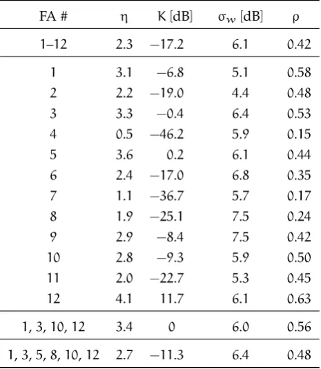
At first, we estimated the channel parameters by applying the lin-ear least squares method (LSM) to all the24 480RSS values collected, obtaining K = −17.2 dB and η = 2.3. The achieved result is shown in Figure 3.2(b)on the preceding page, where the dots represent RSS measurements and the solid line refers to the theoretical path-loss model derived by linear regression. In order to determine if the data well fit the derived parameters, we computed also the regression co-efficientρ, which resulted to be equal to0.42. Moreover, the standard deviation of the RSS measurements wasσw=6.1dB, leading to a rel-ative bias on the estimated distance of 17%, and a relative standard deviation of60%, as given by (3.2) and (3.3), respectively.
Secondly, we analyzed the path-loss model considering each FA node individually, while the MT was still moved in each of the68test points. The channel parametersKandηwere still estimated by using the LSM for each data set of2040collected RSS values.
Then, we considered the four FAs (i.e., FAs1,3,10and12) located in the corners of the room and the six-FA configuration given by the four FAs in the corners and the two FAs (i.e., FAs5and8) in the mid-dle of the room. We collected8160and12 240RSS values, respectively, and as described before, we used these values to estimate the channel parametersηandKthrough the LSM.
Table 3.1 on the following page lists the log-distance channel pa-rameters estimated in each case, together with the error standard de-viation and the related regression coefficient. As shown, the channel-model-error standard deviation is nearly constant for all the consid-ered sets of FAs, whereas the resulting path-loss exponents is quite changing. In particular, considering the channels related to each sin-gle FA, it ranges from a minimum of 0.5 for FA 4 to a maximum of
24 r s s-b a s e d r a n g i n g a n d p o s i t i o n i n g i n i n d o o r e n v i r o n m e n t
Table 3.1: Log Normal Channel Parameters.
FA # η K[dB] σw[dB] ρ
1–12 2.3 −17.2 6.1 0.42
1 3.1 −6.8 5.1 0.58
2 2.2 −19.0 4.4 0.48
3 3.3 −0.4 6.4 0.53
4 0.5 −46.2 5.9 0.15
5 3.6 0.2 6.1 0.44
6 2.4 −17.0 6.8 0.35 7 1.1 −36.7 5.7 0.17 8 1.9 −25.1 7.5 0.24
9 2.9 −8.4 7.5 0.42
10 2.8 −9.3 5.9 0.50 11 2.0 −22.7 5.3 0.45
12 4.1 11.7 6.1 0.63
1,3,10,12 3.4 0 6.0 0.56
1,3,5,8,10,12 2.7 −11.3 6.4 0.48
estimation point of view, these FAs represent the worst and the best case, respectively. Indeed, a higher value of the regression coefficient means that the data received by the related FA carry more informa-tion about the unknown distance. It is worth noticing that the four FAs located in the corners of the room provided the highest value of the regression coefficient; thus, they can be considered as the more informative ones. To the best of our knowledge, no previous work has reported remarkable differences of the channel parameters when considering each FA node singularly. However, given the different po-sitions of the FAs, the received signal is expected to be not affected by the same reflections, fading and multipath interference, thus leading to a significant difference in the channel models. It is worth noticing that similar observations on the irregularity of the wireless commu-nication channel were presented in [41], in which an extension to the isotropic radio model for outdoor environment was proposed.
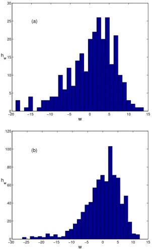
The histograms hw of the RSS errorw are depicted in Figure 3.3 on the next page, for the case of the 4and12 FAs, respectively. Both distributions show a behavior far from Gaussian, which is conversely to the assumption commonly made in the literature [10].
3.3 r f c h a n n e l c h a r a c t e r i z at i o n 25
−200 −15 −10 −5 0 5 10 15
5 10 15 20 25 30
h w
w (a)
−300 −25 −20 −15 −10 −5 0 5 10 15
20 40 60 80 100 120
h
w
w (b)
26 r s s-b a s e d r a n g i n g a n d p o s i t i o n i n g i n i n d o o r e n v i r o n m e n t
obtained histograms noticeably differ each other, suggesting a nonsta-tionary behavior of the RSS error with respect to the distance, which is different from what we would expect from the model suggested in [10].
3.4 l o c a l i z at i o n a l g o r i t h m s
The localization problem can shortly be formalized as follows. Con-sider a set of nodesN= {A1,A2, . . .,An}, each one with a fixed and known position. Note that we are working with the common assump-tion of 2D localizaassump-tion, since the third dimension usually is not of primary interest in indoor environment. Thus, the position of a FA is a two-tuple ai= (xi,yi), wherexi andyiare evaluated with respect to originOof the reference system. Letpdenote the position of a MT node of unknown coordinates (x,y), and let RSSi denote the mea-sured intensity of the signal strength from FAai experienced by the MT. The goal of a RSS-based localization algorithm is to provide esti-mate ˆp= (xˆ, ˆy)of positionpgiven the vector[RSS1,RSS2, . . .,RSSn]. RSS-based positioning algorithms can be categorized into two classes [27,42]:
• the range-based algorithm, which use several target-to-anchor distance estimations obtained through the RSS measurements to determine the position of the MT node;
• the range-free algorithm, which determines the position of the MT node without performing distance estimation.
In the following, we analyze two different approaches, the WCL and the REWL, respectively. The former belongs to the class of range-based solutions, whereas the latter is a range-free method. Both al-gorithms are characterized by a low computational effort. This, com-bined with low transmission power, allows to significantly limit node energy consumption.
3.4.1 Weighted Centroid Localization
es-3.4 l o c a l i z at i o n a l g o r i t h m s 27
tablished during the measurement. More specifically, the estimated position of the MT node is given by:
ˆ
p= 1
m·
m
X
i=1
ai (3.5)
wherem is the cardinality of the subsetN of visible FAs. It is worth noticing that when the MT node communicates with all the FAs, i.e., all FAs are visible, the centroid results the center of the FAs coordi-nates. Notice that the CL approach assumes all the visible FAs equally near the MT node. Since this assumption is most likely not satisfied in practice, in [44], the introduction of a function which assigns a greater weight to the FAs closest to the target, was proposed. The result is the WCL algorithm, which estimates the position of the MT node as:
ˆ
p=
n
X
i=1
(dˆi−g·ai) n
X
i=1 (dˆi−g)
(3.6)
where ˆdi is the distance between the MT and FA ai, which is esti-mated through RSSi of the visible FAs. Exponent g > 0determines the weight of the contribution of each FA. If g = 0, then ˆpis simply the sample mean of ai, and the WCL reduces to the CL approach. Increasing the value of g causes the FAs to reduce the range of their “attraction field” with respect to the MT node, thus increasing the
relative weight of the nearest FAs.
28 r s s-b a s e d r a n g i n g a n d p o s i t i o n i n g i n i n d o o r e n v i r o n m e n t
Similar error surfaces were obtained assuming that additive white Gaussian noise (AWGN) with different values of standard deviation affects the RSS measurements. We noticed that, on average, the max-imum values of the algorithm error are little sensitive to the noise. Otherwise, the noise affects significantly areas with small error val-ues, usually located near the center of the room, therefore increasing the center clustering behavior of the algorithm.
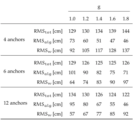
Table 3.2and3.3 on page31show the mean and root-mean square (RMS) values of the total distance error in the estimated positionetot, which is achieved by running the WCL algorithm on the experimen-tal data, with 4, 6 and 12 anchors, and considering different values of the exponent gwithin the range (1.0, 1.8). In particular, the algo-rithm inputs were the distances between the MT and each FA, which are estimated by inverting (3.1) and using the RSS values measured in each of the 68test points, as described inSection 3.2andSection 3.3. The same Tables also summarize the mean and the RSS of the algo-rithm distance error ealg and the experimental noise distance error
ewdetermined for the same sets of FAs and values of the exponentg. The experimental noise distance error was obtained as the difference between the position estimates determined by running the WCL al-gorithm using both the true and estimated distances. Notice that this latter error is due to the noise componentwin (3.1). In particular, Ta-ble 3.2and3.3show that, on the first approximation, meanµalg and
RMSalg of the algorithm error depend little on the FA position (i.e., FA number) and decrease with a raising exponentg. This behavior is partially compensated by the noise error, whose meanµwandRMSw
values increase with an increasing value ofgand decrease with a rais-ing number of FAs. As a result, the effect of the algorithm error on the total error is negligible for the four FAs, while it counts for6and
12FAs.
Furthermore, considering any two different FA configurations (e.g.,
4 and12 FAs) it is interesting to note that the ratio of the correspon-dent mean µw and RMS RSSw values of the noise error reported in
Table 3.2and3.3 tend to be inversely proportional to the square root of the product between the number of FAsnand the regression coef-ficientρgiven inTable 3.1on page 24, i.e.,
µw∝
s
1
3.4 l o c a l i z at i o n a l g o r i t h m s 29
170217
264311
358405
451498545
592639 216 262 307 353 399 445 490 536 0 20 40 60 80 100 120 140 (a) [cm] [cm] ealg [cm] 10 20 30 40 50 60 70 80 90 170217 264311 358405 451498 545592 639 216 262 307 353 399 445 490 536 0 20 40 60 80 100 120 140 (b) [cm] [cm] ealg [cm] 20 40 60 80 100 120 170217 264311 358405
451498545
592639 216 262 307 353 399 445 490 5360 20 40 60 80 100 120 140 (c) [cm] [cm] ealg [cm] 10 20 30 40 50 60 70
30 r s s-b a s e d r a n g i n g a n d p o s i t i o n i n g i n i n d o o r e n v i r o n m e n t
and
RMSw∝
s
1
n·ρ (3.8)
Since a growing number of FAs results in a decrease in the regres-sion coefficient, using more FAs reduces the effect of noise by a factor that is smaller than the square root of the number of FAs. In any case, (3.7) and (3.8) can provide some useful hints on the expected effect of noise in different system configurations with changing number of FAs.
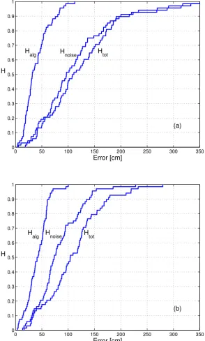
Figure 3.5on page 33 depicts the cumulative histograms H of the WCL estimation errors considering the four FAs in the corners of the room and all the 12 FAs. As expected, the median total estimation error is about 1m using both 4 or 12 FAs. Indeed the 4 FAs in the corners carry most of the information about the unknown distance, as shown inSection 3.3. Notice also that the use of12FAs, although does not produce a significant reduction of the average estimation error, has a beneficial effect on the maximum error.
3.4.2 Relative Span Exponential Weighted Localization
The REWL is an RSS-based range-free localization algorithm recently proposed in the literature [45]. This algorithm is inspired by the WCL method. The weights are obtained by the relative placement of each FA RSS value within the span of all the RSS values measured by the MT node. In the estimation of the MT position, the REWL algo-rithm favors the FAs which exhibit higher RSS values and therefore are likely to be closer to the MT node. This is obtained using the weighting factor λ, according to the exponentially moving average concept [45]. The estimated MT node position is given by [45]
ˆ
p=
n
X
i=1
[(1−λ)RSSmax−RSSi×a
i] n
X
i=1
(1−λ)RSSmax−RSSi
(3.9)
3.4 l o c a l i z at i o n a l g o r i t h m s 31
Table 3.2: WCL Algorithm Mean Distance Error.
g
1.0 1.2 1.4 1.6 1.8
4 anchors
µtot[cm] 113 113 116 120 124
µalg[cm] 67 52 42 38 40
µw[cm] 78 89 99 107 114
6 anchors
µtot[cm] 116 112 110 109 110
µalg[cm] 94 83 75 69 64
µw[cm] 55 63 71 78 84
12 anchors
µtot[cm] 123 117 114 111 109
µalg[cm] 87 73 60 50 41
µw[cm] 50 59 68 76 83
Table 3.3: WCL Algorithm RMS Distance Error.
g
1.0 1.2 1.4 1.6 1.8
4 anchors
RMStot[cm] 129 130 134 139 144
RMSalg[cm] 73 60 51 47 46
RMSw[cm] 92 105 117 128 137
6 anchors
RMStot[cm] 129 126 125 125 126
RMSalg[cm] 101 90 82 75 71
RMSw[cm] 64 74 83 90 97
12 anchors
RMStot[cm] 134 130 126 124 122
RMSalg[cm] 95 80 67 55 46
32 r s s-b a s e d r a n g i n g a n d p o s i t i o n i n g i n i n d o o r e n v i r o n m e n t
REWL algorithm reduces to (3.6), wheregranges between0.5and3.9
whenη andλassume values in (1, 4)and(0.1, 0.2) intervals, respec-tively (as given in the Appendix A).
Figure 3.6 on page 35 shows the surfaces representing the algo-rithm distance error ealg, which is obtained by running simulations of the REWL algorithm forλ=0.15, with4,6, and12FAs and with a grid resolution of5cm. The inputs of the algorithm were the theoreti-cal RSS values that might be measured by the MT in each point of the grid in the absence of noise. These values were evaluated using the path-loss model (3.1), considering for each set of anchors the related channel parameters η and K reported in Table 3.1 on page 24 and the true distances d between the MT and the FAs, which are calcu-lated from their known coordinates. The transmission power was as-sumed to bePtx = −25dB, and the reference distance wasd0 =10cm. Clearly, the error tends to decrease with the increasing number of FAs. The shape of the error surfaces is substantially similar to the one of the WCL algorithm, with the exception of the four-FA configuration that features an higher error around the center of the grid. As pre-viously highlighted for the WCL, the six-FA configuration exhibits higher algorithm error values with respect to the four-FA configura-tion. Moreover, we analyzed also the error surfaces obtained by as-suming the RSS values affected by AWGN. Assessment on these is similar to the ones drawn for the WCL algorithm.
Table 3.4and3.5on page34report the mean and RMS values of the total distance error in the estimated positionetot, which is achieved by running the REWL algorithm with 4,6, and12 FAs and consider-ing λ = 0.10, λ = 0.15, and λ= 0.20. The algorithm inputs were the RSS values measured by the MT node in each of the68test point, as described inSection 3.2and3.3. The same Tables show also the mean and RMS values of the algorithm distance errorealg and the experi-mental noise distance errorew. This latter error is determined as the difference between the position estimates achieved by running the REWL algorithm on both the theoretical and measured RSS values. As shown, meanµalgandRMSalgof the algorithm error depend on the number of FAs, but they feature a different behavior as the weight-ing factorλchanges. In fact, with four FAs they increase passing from
3.4 l o c a l i z at i o n a l g o r i t h m s 33
0 50 100 150 200 250 300 350 0
0.1 0.2 0.3 0.4 0.5 0.6 0.7 0.8 0.9 1
Error [cm] H
(a) H
alg Hnoise Htot
0 50 100 150 200 250 300 350
0 0.1 0.2 0.3 0.4 0.5 0.6 0.7 0.8 0.9 1
Error [cm] H
(b) H
alg Hnoise Htot
Figure 3.5: Cumulative histograms for the WCL localization algorithm er-rors considering(a) the 4 FAs in the corners of the room, and
34 r s s-b a s e d r a n g i n g a n d p o s i t i o n i n g i n i n d o o r e n v i r o n m e n t
Table 3.4: REWL Algorithm Mean Distance Error.
λ
0.10 0.15 0.20
4 anchors
µtot[cm] 111 114 125
µalg[cm] 38 58 77
µw[cm] 95 117 130
4 anchors
µtot[cm] 116 106 105
µalg[cm] 82 62 59
µw[cm] 56 76 91
12 anchors
µtot[cm] 127 113 105
µalg[cm] 83 49 30
µw[cm] 51 75 92
Table 3.5: REWL Algorithm RMS Distance Error.
λ
0.10 0.15 0.20
4 anchors
RMStot[cm] 127 131 144
RMSalg[cm] 47 59 82
RMSw[cm] 111 138 157
6 anchors
RMStot[cm] 130 121 120
RMSalg[cm] 89 69 65
RMSw[cm] 69 91 107
12 anchors
RMStot[cm] 139 126 120
RMSalg[cm] 91 54 33
3.4 l o c a l i z at i o n a l g o r i t h m s 35
170217
264311
358405
451498545
592639 216 262 307 353 399 445 490 536 0 20 40 60 80 100 120 140 (a) [cm] [cm] ealg [cm] 10 20 30 40 50 60 70 80 90 170217 264311 358405 451498 545592 639 216 262 307 353 399 445 490 536 0 20 40 60 80 100 120 140 (b) [cm] [cm] ealg [cm] 20 40 60 80 100 120 170217 264311 358405
451498545
592639 216 262 307 353 399 445 490 5360 20 40 60 80 100 120 140 (c) [cm] [cm] ealg [cm] 10 20 30 40 50 60 70 80
Figure 3.6: REWL distance error forλ=0.15considering(a)the4FAs in the corners of the room,(b)6FAs, and(c)all the12FAs reported in
36 r s s-b a s e d r a n g i n g a n d p o s i t i o n i n g i n i n d o o r e n v i r o n m e n t
total error, they depend little on both the FA position (i.e., FA number) and the weighting factorλ.
Figure 3.7shows the cumulative histograms H of the localization errors resulting when running the REWL algorithm withλ=0.15and for the four FAs on the corners of the room and for all 12 FA nodes, respectively. Considerations similar to those expressed for the WCL algorithm can be done. In particular, for the 12-FA configuration, the maximum total distance error etot is limited, while the algorithm distance errorealgis not negligible.
3.5 c o n c l u s i o n
In this Chapter, we have analyzed the performance of indoor rang-ing and positionrang-ing based on RSS measurements collected by a WSN. The accuracy of two classes of low-computational-effort positioning algorithms relying on the centroid concept, which are called WCL and REWL, has been investigated. The measurement system was de-ployed in a real indoor environment where, by the online running of the studied algorithms, we obtained the estimated position of a MT node in different test points inside an observation field.
At first, we characterized the indoor wireless propagation channel using the log-distance shadowing path loss model, which is largely adopted in the literature. We showed that this model is affected by a quite high relative bias and standard uncertainty. This is most likely due to the severe propagation conditions of the indoor radio channel, i.e., affected by multipath and shadowing phenomena. Therefore, we might expect that the ranging error and, as a consequence, the MT positioning error grows as the distance from the FAs increases.
Secondly, we found that the information carried by each FA strongly depends on the FA position. Hence, for both the considered position-ing algorithms, an increasposition-ing number of FAs does not necessarily improve measurement accuracy, i.e., conversely to what we would expect.
asso-3.5 c o n c l u s i o n 37
0 50 100 150 200 250 300 350
0 0.1 0.2 0.3 0.4 0.5 0.6 0.7 0.8 0.9 1
Error [cm] H
(a) H
alg Hnoise Htot
0 50 100 150 200 250 300 350
0 0.1 0.2 0.3 0.4 0.5 0.6 0.7 0.8 0.9 1
Error [cm] H
(b)
Halg H
noise Htot
38 r s s-b a s e d r a n g i n g a n d p o s i t i o n i n g i n i n d o o r e n v i r o n m e n t
ciated to the wireless propagation channel model and, in any case, it results as high as few tens of percent of the size of the considered indoor environment.
4
HYBRID RSS-RTT METHOD FOR RANGING PERFORMANCE IMPROVEMENT
4.1 i n t r o d u c t i o n
T
he study we carried out in Chapter 3 highlighted the consid-erable sensitivity of the RSS-based ranging and positioning to multipath and shadowing phenomena. In particular, the multipath propagation alters the relationship between RSS values and distance described by the log-distance shadowing path loss model (2.3), and yields to non-monotonic and space-varying measurement results. Ap-parently, the RSS values exhibit large space-varying fluctuations, but a quite small variance over time when the receiving and the transmit-ting devices are still and the environment is not perturbed by other moving objects. Despite these limitations, the wide availability of wireless transceiver chips equipped with RSSI makes the RSS-based ranging an easy and cost-effective means to enable object positioning in indoor environment.On the other hand, as mentioned in Chapter 2, the distance be-tween two wireless devices can be derived from the signal ToF ob-tained by means of RTT measurement. It is worth reminding that the RTT is measured by the same device, so no common time reference between transmitter and receiver is needed. Therefore, the RTT-based approach eliminates the error due to imperfect time synchronization between the devices. The ranging accuracy in this case depends on a variety of factors, such as the signal modulation type, the properties of the adopted transceiver and the timestamping mechanisms at the transmitting and receiving ends, i.e., the technique used to record the moment when a message is whether sent or received [46].
All things considered, by leveraging the possibility of combining different measurements by means of multisensor data fusion
tech-Parts of this Chapter are going to appear in:
D. Macii, A. Colombo, P. Pivato, and D. Fontanelli, “A Data Fusion Technique for Wireless Ranging Performance Improvement,”IEEE Transactions on Instrumentation and Measurement, vol. 61, no. 1, pp. 27–37, Jan. 2013.