Mathematical Modeling with Local Volatility Surface by Radial Basis Function Approach

Vol. 9, No. 2, 2015, 191-200

ISSN: 2279-087X (P), 2279-0888(online) Published on 14 March 2015

www.researchmathsci.org

191

Annals of

Mathematical Modeling with Local Volatility Surface by

Radial Basis Function Approach

Lasker Ershad Ali1, Masudul Islam2 and Shamima Sultana1

1

Mathematics Discipline, Khulna University, Khulna-9208, Bangladesh

E-mail: [email protected]

2

Statistics Discipline, Khulna University, Khulna-9208, Bangladesh

E-mail: [email protected]

Corresponding author: Lasker Ershad Ali

Received 18 February 2015; accepted 3 March 2015

Abstract. Some obstacles create vulnerable situations in financial market. Overcome this

unexpected situation, it is essential to reform the financial market by measuring the risk of share market. This project investigates the sensitivity of radial basis functions to construct different volatility surface by radial basis function approaches to understand the risk of share market. Different types of radial basis functions on the basis of different error measurement such as average error as well as relative average error of Dhaka Stock Exchange (DSE) are measured and multiquadratic function gives the best result with compare to other functions especially Gaussian and Thin plate spline function.

Keywords: Financial market, radial basis function, volatility surface AMS Mathematics Subject Classification (2010): 34K28, 34K50, 34K60 1. Introduction

Stock market is one of the principal financial institutions of Bangladesh which opens door for companies to raise huge amount of capital from a lot of individual investors inside and outside of the country. To observe the present situation of the market and to find the volatility surface we use radial basis function with some interpolation and also try to introduce different Radial basis functions such as Gaussian function, multi-quadratic function and thin plane spline function to evaluate observations.

192

In the early 1970s, Fischer Black, Myron Scholes, and Robert Merton made a major breakthrough in the pricing of stock options [1]. The famous Black-Scholes model has been intensively studied and used as the foundation for almost any option pricing formula in today’s financial markets. The model has a huge influence on the way that trader’s price and hedge options [15]. It has also been pivotal to the growth and success of financial engineering in the 1980s and 1990s. Here shows the Black-Scholes model for valuing Bangladeshi call and put options on a non dividend paying stock is derived. In 1987 Hull and White explained the pricing of options on assets with stochastic volatilities [10]. Hon and Mao used radial basis function method for solving options pricing model in 1999 [9]. Coleman and Verma reconstructed the unknown local volatility function for options pricing model also in 1999 [3]. Recently, many researchers working in the field of financial mathematics especially radial basis functions approaches to observe share market situation. In 1999, Schaback improved error bounds for scattered data interpolation by radial basis functions [13] and solved limit problems for interpolation by analytic radial basis functions in 2008. Driscoll, and Fornberg described interpolation problem in the limit of increasingly flat radial basis functions [4]. Kim, et al. reconstructed local volatility function approximation by using radial basis function networks in 2006 [11]. In 2010, Glover used radial basis function approach to reconstructing the local volatility surface of European options [7].

This paper can be explained how volatility can be either estimated from historical data or implied from option prices using the model and show how the Black-Scholes model can be extended to deal with Bangladeshi call and put options on dividend-paying stocks and present some results on the pricing of Bangladeshi call options on dividend paying stocks.

2. Some mathematical tools

The derivation of the Black-Scholes partial differential equation (PDE) is based on the fundamental fact that the option price and the stock price depend on the same underlying

source of uncertainty. If Sis asset price,

σ

is volatility, r is risk free rate and V(S,t)

the price of a derivative as a function of time and stock price then Black-Scholes partial differential equation [1] is

2 2

2 2

2 1

S S

V t

V rS S V

rV

σ

∂ ∂ + ∂ ∂ + ∂ ∂

= (1)

The boundary conditions can be easily determined by the option price. For a call option at expiry the option is worth the difference between the current underlying asset price S and the strike price K, if S > K the call boundary condition is

) 0 , max(S K

VT = T − (2)

where, S_Tis the asset price at maturity T. Again, a similar argument can be used for a put

option resulting in the put boundary condition

) 0 ,

max( T

T K S

V = − (3)

The Black-Scholes equation shows that inputs required for modeling an option are the underlying asset price S, the strike K, the maturity T, the risk free rate r, and the

volatility all these parameters are directly observable except for the volatility. The

193

) ( ) (x

φ

x

φ

= is the RBF so that

φ

acts on a vector in Rn space and only through the

norm. This means that

φ

can be thought a scalar function. The radial basis functions as

the model functions is f(x)=

α

1

φ

(

x−x1

)

+...+

α

_p

φ

(

x−x_p

)

(4)

where

φ

:R+ →R is typically nonlinear and is referred to as the transfer function [13].

Three types of radial basis functions like Gaussian, thin plate, and multiquadric are chosen for the model setup. RBF represents a map from P-dimensional input space to the

one-dimensional output space i.e. f :Rp →R1 that consists of a set of weights

m i i

w 1 ) (

}

{ ₌ and a set of radial basis functions mi

i

g 1 ) (

}

{ ₌ wherem≤n. There is a large class

of radial basis functions which can be written in a general form

(

()

)

) ( )

(

)

( i i

i

c x x

g =

φ

− (5)

where . denotes the Euclidean norm and {c(i)}_im₌₁ is a set of the centers that can be

chosen from the data points. For function approximation here uses Multiquadric function

approximation

φ

(i)(r)=

(

x−c(i)

)

= r2 +a(i)2 for somea(i) >0 (6) Inverse multiquadric approximation and Gaussiann function approximation respectively.

(

()

)

_{2 ()2}

)

( 1

) (

i i

i

a r c

x r

+ = − =

φ

for somea(i) >0 (7)

(

)



  

 

− = −

= () ₍2₎₂

) (

exp )

( i _i

i

a r c

x r

φ

for somea(i) >0 (8)

where a(i) is usually referred to as the width of the th basis function and

r= x−c(i) =

(

x−c(i)

)(

.x−c(i)

)

.

Here multivariate interpolation is used for reconstruct volatility surface. Thus the

simplest case of reconstruction of a d-variate unknown function u* from data occurs

when only a finite number of data in the form of values ( ),..., *( )

1 *

m

x u x

u at

arbitrary locations x ,...,1 xm in

d

R forming a set X ={x1,...,xm} are known. In

contrast to the n trial points y ,...,₁ y_n is

(

2

)

1

)

( _k

n

k

k x y

x

u =

∑

−

=

φ

α

(9)

The m data locations x ,...,₁ x_m are called test points or collocation points. To calculate

a trial function u of the form (9) which reproduces the data ( 1),..., *( )

*

m

x u x

u well,

we have to solve the m×nlinear system

(

xi yk

)

u xi i m

n

k

k − ≈ < <

∑

=

1 ), (

* 2 1

φ

α

(10)

for n coefficients

α

₁,...,

α

_n matrices with entries

φ

(

x_i−y_{k 2}

)

will occur and they are

194

sense to reconstruct u* by a function u of the form (9) by enforcing the exact

interpolation conditions

(

x x

)

j m n

x

u j k

n

k k

j =

∑

− ≤ ≤ =

= 1 , ) ( 2 1 *

α

φ

(11)

This is a system of m linear equations in m=n unknowns

α

1,...,

α

_n with a

symmetric coefficient matrix

(

)

(

j k

)

_{j k m}

x x x

A ≤ ≤ − = , 1 2

φ

(12)

In general, solvability of such a system is a serious problem, but one of the central features of kernels and radial basis functions is to make this problem.

3. The model

Reconstructing the local volatility surface is using for radial basis functions and the advance taken in the paper follows that of [7] closely, except radial basis functions are used instead of spline to represent the local volatility function. That is, a function

= ∑

=

m

j j j

h w t S 1 ) , (

σ

(13)

with h a set of m radial basis functions and

j

w a set of corresponding weights found that

satisfies ) , ( min t S

σ

∑₌ − n i f v t S i v

i 1 BS

2 )] ( )) , ( (

[

σ

(14)

where ( )

i f v

BS is the set of observed Black-Scholes prices and vi(

σ

(S,t)) is the

option price at S and t are given by

2 2 2 2 ) , ( 2 1 S t S S V t V rS S V rV

σ

∂ ∂ + ∂ ∂ + ∂ ∂

= (15)

The generated surfaces suffer from over fit and become unstable. To reduce this unstable condition, Tikhonov regularization can be used for this problem

) , ( min t S

σ

∑₌ − + ∑₌ m j j i BS w n i f v t S i v 1 1 2 )] ( )) , ( (

[

σ

λ

(16)

Equations (14) and (16) are nonlinear least squares minimization problems. A number of simplifying assumptions and heuristics are used to reduce the scale of the optimization presented in equation (14). Firstly we assume that the set of m radial basis functions, h in equation (13) are known and their positioning (centers) are fixed. The range of function sets are used and try to establish the best choice for the local volatility problem. The result of this assumption is to reduce the optimization problem to find the optimal weight

vector . Secondly we assume that, if Tikhonov regularization is needed then the

regularization parameter

λ

is chosen by using trial and error methods which are found

195

project. The procedure to recover the local volatility function for the problem is presented below for each of the key steps. For the function set h with observed market data f then

(i) Find an initial weight vectorw₀.

(ii) Evaluate the cost function given in equation (14)

(iii) Using an optimization algorithm update the optimal weight vector.

The whole procedure is very sensitive to initial choice of weight vector. To solve this and generate a surface of realistic volatilities a simple method is used. To find an

initialw₀such that the implied volatilities of observed market data f are interpolated using

the appropriate radial basis function set h and solve the following equation,

0

min

w ∑

( )

_ + ∑ 

   

∑

−

= = =

n

j m

w i

x h m

w i

f

i j

j j

1 1

2

0 2

1

0

λ

(17)

This provides an initial weight vector 0

w that gives a volatility surface that is reasonable.

Nelder-Mead Simplex Optimization algorithm is used as an optimization algorithm. The basic idea behind the Nelder-Mead Simplex algorithm is the creation and evolution of a simplex of points on the cost function surface to find the minimum. A simplex is a

prototype with n+1vertices in n dimensions. The vertices of this prototype are evaluated

and adjusted using several simple rules depending on the geometry of the function being searched. The first stage of the Nelder-Mead algorithm is creating the simplex.

For the implementation of this project the Preconditioned Conjugate Gradient approach [7] is used and the optimization algorithms for purposes of efficiency and simplicity it is decided that implementations in the MATLAB optimization toolbox would be used. The data which are used in this research obtained from Dhaka Stock Exchange and collect information about different strikes and different maturity rates from Bangladesh Bank. All data which are used in this research are secondary data.

4. Results and discussions

The basic problem of scientific computing that recovers the multivariate functions from discrete data. For this purpose we use radial basis functions and confine to reconstruct from strong data consisting of evaluations of the function itself or its derivatives at discrete points. Using 258 data to recover the functions from data sets are given as integrals against the test functions which are the challenging research problems [12].

0 50 100 150 200 250 300

-1 0 1 2 3 4 5 6 7

Different Radial Basis Function

Days of Index Data

E

x

p

e

c

ta

ti

o

n

V

o

la

ti

lit

y

Gaussain Function Multi quardic Function Thin plate spline Function

196

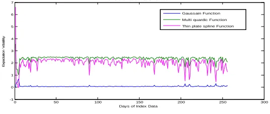
The above figure shows the different radial basis functions like Gaussian, multiquadratic and thin plate spline. It shows that the Gaussian function is better than other radial basis functions. Now investigate the errors for radial basis functions.

0 50 100 150 200 250 300

3000 3200 3400 3600 3800 4000 4200 4400 4600

Deys of Index Data

E

x

p

e

c

ta

ti

o

n

A

v

e

ra

g

e

E

rr

o

r

Average Error For Different Radial Basis Function Gaussain Average Error

Multi quardic Average Error Thin plate spline Average Error

Figure 2: Average error for different radial basis functions

The figure (2) shows average error for the different type of radial basis functions by using 258 data. It shows that all types of radial basis functions are overlapping each other. So it can’t identify the best for minimizing the error.

0 50 100 150 200 250 300

0.9975 0.998 0.9985 0.999 0.9995 1

1.0005 Relative Average Error For Different Radial Basis Function

Days of Index Data

E

x

p

e

c

ta

ti

o

n

R

e

la

ti

v

e

E

rr

o

r

Gaussain Relative Average Error Multi quardic Relative Average Error Thin plate spline Relative Average Error

Figure 3: Relative average error for different radial basis functions

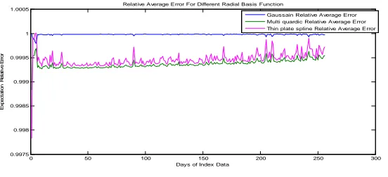
The above figure shows the relative average error for the different type of radial basis functions for 258 data and the multiquadratic function is best from other radial basis functions.

For the purposes of comparison, we use the same test problems presented in [7], [12] and several measures of performance are used for consistency. Firstly the average absolute error at each of the n known data points in pricing is given by

∑

= −

= n

i i

f i

V n ₁ ( )

1 error

Average

σ

(18)

where (

σ

)

i

V is the price at the data point i and

i

f is the observed radial basis function.

The maximum absolute error is observed at the data points for the equation (8).Then

interpolation is also given by

n i

i f i

V ( ) 1,...,

Max error

Max =

σ

− ∀ = (19)

∑

=

−

= n

i f_i i f i

V

n ₁

) ( 1

error relative Average

σ

197

i n

i f

i f i

V

,..., 1 )

( Max error relative

Max ∀ =

  

 

  



 ₋

=

σ

(21)

This research examines the radial basis interpolating function to reconstruct the surface and to judge the smoothness according to radial basis optimization algorithm. The radial basis function approach is running to use local volatility by the Nelder-Mead optimization, with Gaussian, multiquadratic and thin plate spline function sets are presented in table (1).

Radial Basis Function

Average Absolute Error

Maximum Absolute Error

Average Relative Error

Maximum Relative Error

General 3809.191 4612.344 0.999597 0.999998

Gaussian 3810.291 4612.648 0.999893 1.000000

Multiquadratic 3809.075 4610.683 0.999565 0.999881

Thin plate spline 3809.444 4611.504 0.999651 1.000023

Table 1: Summarized result using Nelder-Mead algorithm

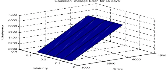
By using the equation (18) and the values from the table (1), we get different figures of Gaussian average error by using MATLAB code whose are shown in the figures bellow.

3000

3500

4000

4500 0

0.1 0.2 0.3 0.4 3000 3200 3400 3600 3800 4000 4200

Strike Gaussian average Error for 15 days

Maturity

V

o

la

ti

lit

y

e

rr

o

r

Figure 4: Gaussian average error for 15 days using Nelder-Mead algorithm

3000

3500

4000

4500

0 0.1 0.2 0.3 0.4

0 0.5 1 1.5 2

V

o

la

ti

lit

y

e

rr

o

r

Gaussian Relative Average Error for 15 days

Strike Maturity

198

3000

3500

4000

4500 0

0.1 0.2 0.3 0.4 2800 3000 3200 3400 3600 3800 4000

Strike Multiquadratic Average Error for 15 days

Maturity

V

o

la

ti

lit

y

e

rr

o

r

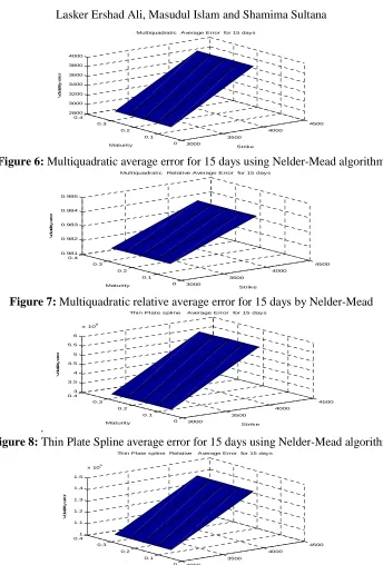
Figure 6: Multiquadratic average error for 15 days using Nelder-Mead algorithm

3000

3500

4000

4500 0

0.1 0.2 0.3 0.4 0.981 0.982 0.983 0.984 0.985

Strike Multiquadratic Relative Average Error for 15 days

Maturity

V

o

la

ti

lit

y

e

rr

o

r

Figure 7: Multiquadratic relative average error for 15 days by Nelder-Mead

. 3000

3500

4000

4500 0

0.1 0.2 0.3 0.4

3 3.5 4 4.5 5 5.5 6

x 108

Strike Thin Plate spline Average Error for 15 days

Maturity

V

o

la

ti

lit

y

e

rr

o

r

Figure 8: Thin Plate Spline average error for 15 days using Nelder-Mead algorithm

3000

3500

4000

4500 0

0.1 0.2 0.3 0.4

1 1.1 1.2 1.3 1.4 1.5

x 105

Strike Thin Plate spline Relative Average Error for 15 days

Maturity

V

o

la

ti

li

ty

e

rr

o

r

Figure 9: Thin Plate Spline relative average error for 15 days using Nelder-Mead

algorithm

199

defined surfaces which closely resemble the known volatility function or both the thin plate spline and the multiquadratic and a very unstable surface for the Gaussian.

In this research we try to find the minimum error among different types of radial basis function. In figure (1) we get three different types of curves of radial basis functions. But it is difficult to measure which is the best function. That’s why, we consider radial basis function in term of average error which are shown in figure (2) but face some problem to understand which function is the best. So we use relative average error for different radial basis function and get the best result for minimization the error for multiquadratic function which shown in figure (3).

Again we go for numerical solution to find the absolute error. From table (1) the average absolute error for general radial basis function is 3809.191, the maximum absolute error for general radial basis function is 4612.344, the average relative error for general radial basis function is 0.999597 and the maximum relative error for general radial basis function is 0.999998. The average absolute error for Gaussian radial basis function is 3810.291, the maximum absolute error for Gaussian radial basis function is 4612.648, the average relative error for Gaussian radial basis function is 0.999893 and the maximum relative error for Gaussian radial basis function is 1. The average absolute error for multiquadratic radial basis function is 3809.075, the maximum absolute error for multiquadratic radial basis function is 4610.683, the average relative error for multiquadratic radial basis function is 0.999565and the maximum relative error for multiquadratic radial basis function is 0.999881. The average absolute error for Thin plate spline radial basis function is 3809.444, the maximum absolute error for Thin plate spline radial basis function is 4611.504, the average relative error for Thin plate spilne radial basis function is 0.999651 and the maximum relative error for Thin plate spline radial basis function is 1.000023. Comparing the results both Thin plate spline and multiquadratics perform well, but Gaussian function sets not perform satisfactory level. So, more accurate result has shown by using the multiquadratic radial basis function. Thus multiquadratic radial basis function gives more accurate result than other two radial basis function in terms of error.

5. Conclusion

200

Acknowledgements

This research work has been supported by Khulna University Research Cell, Bangladesh. Therefore we have expressed our gratefulness to Khulna University Research Cell for the financial support.

REFERENCES

1. F.Black and M.Scholes, The pricing of options and corporate Liabilities, Journal of

Political Economy, 81(4) (1973) 637-654.

2. J.B.Cherrie, R.K.Beatson and G.N.Newsam Fast evaluation of radial basis functions:

methods for generalized multiquadrics inRn, SIAM Journal on Scientific Computing,

23 (5) (2002) 1549–1571.

3. F.Coleman, Y.Li and A.Verma, Reconstructing the unknown local volatility function,

Journal of Computational Finance, 2(3) (1999) 77-102.

4. T.A.Driscoll and B.Fornberg, Interpolation in the limit of increasingly flat radial

basis functions, Computers & Mathematics with Applications, 43(3–5) (2002) 413– 422.

5. G.E.Fasshauer, Solving differential equations with radial basis functions: multilevel

methods and smoothing, Journal of Advances in Computational Mathematic, 11(2-3) (1999) 139–159.

6. C.Franke and R.Schaback, Solving partial differential equations by collocation using

radial basis functions, Journal of Applied Mathematics and Computation, 93 (1) (1998) 73–82.

7. J.Glover, A radial basis function approach to reconstructing the local volatility

surface of European options. Master thesis of the University of the Witwatersrand, Johannesburg, (2010).

8. R.L.Hardy, Multiquadric equations of topography and other irregular surfaces,

Journal of Geophysical Research, 76 (1971) 1905–1915.

9. Y.C.Hon and X.Z.Mao, A radial basis function method for solving options pricing

mode, Financial Engineering, 8 (1999) 31–49.

10. J.Hull and A.White, The pricing of options on assets with stochastic volatilities.

Journal of Finance, 42(2) (1987) 281-300.

11. H.Kim, D.Lee and J.Lee, Local volatility function approximation using reconstructed

radial basis function networks, Lecture Note of Computer Science 3973, Springer

(2006) 524-530.

12. E.Larsson and B.Fornberg, A numerical study of some radial basis function based

solution methods for elliptic PDEs, Computers & Mathematics with Applications, 46(5-6) (2003) 891–902.

13. R.Schaback, Improved error bounds for scattered data interpolation by radial basis

functions, Mathematics of Computation, 68 (225) (1999) 201–216.

14. M.Pal, Numerical analysis for scientists and engineers: theory and C programs,

Alpha Science International Limited, 2007.

15. D.K.Biswas and S.C.Panja, Advanced optimization technique, Annals of Pure and

Applied Mathematics, 5(1) (2013) 82-89.

16. W.Ritha and I.A.Vinoline, Optimization of EPQ inventory models of two level trade

credit with payment policies under cash discount, Annals of Pure and Applied