Subgroup Discovery with CN2-SD

(1)

Subgroup Discovery with CN2-SD

Nada Lavraˇc [email protected]

Joˇzef Stefan Institute Jamova 39

1000 Ljubljana, Slovenia and Nova Gorica Polytechnic Vipavska 13

5100 Nova Gorica, Slovenia

Branko Kavˇsek [email protected]

1000 Ljubljana, Slovenia

Peter Flach [email protected]

University of Bristol Woodland Road

Bristol BS8 1UB, United Kingdom

Ljupˇco Todorovski [email protected]

1000 Ljubljana, Slovenia

Editor: Stefan Wrobel

Abstract

This paper investigates how to adapt standard classification rule learning approaches to subgroup discovery. The goal of subgroup discovery is to find rules describing subsets of the population that are sufficiently large and statistically unusual. The paper presents a subgroup discovery algo-rithm, CN2-SD, developed by modifying parts of the CN2 classification rule learner: its covering algorithm, search heuristic, probabilistic classification of instances, and evaluation measures. Ex-perimental evaluation of CN2-SD on 23 UCI data sets shows substantial reduction of the number of induced rules, increased rule coverage and rule significance, as well as slight improvements in terms of the area under ROC curve, when compared with the CN2 algorithm. Application of

CN2-SD to a large traffic accident data set confirms these findings.

Keywords: Rule Learning, Subgroup Discovery, UCI Data Sets, Traffic Accident Data Analysis

1. Introduction

(2)

learning is a form of descriptive induction (non-classificatory induction or unsupervised learning), aimed at the discovery of individual rules which define interesting patterns in data.

Descriptive induction has recently gained much attention of the rule learning research commu-nity. Besides mining of association rules (e.g., the APRIORI association rule learning algorithm (Agrawal et al., 1996)), other approaches have been developed, including clausal discovery as in the CLAUDIEN system (Raedt and Dehaspe, 1997, Raedt et al., 2001), and database dependency discovery (Flach and Savnik, 1999).

1.1 Subgroup Discovery: A Task at the Intersection of Predictive and Descriptive Induction

This paper shows how classification rule learning can be adapted to subgroup discovery, a task at the intersection of predictive and descriptive induction, that has first been formulated by Klösgen (1996) and Wrobel (1997, 2001), and addressed by rule learning algorithms EXPLORA (Klösgen, 1996) and MIDOS (Wrobel, 1997, 2001). In the work of Klösgen (1996) and Wrobel (1997, 2001), the problem of subgroup discovery has been defined as follows: Given a population of individuals and a property of those individuals we are interested in, find population subgroups that are statistically ‘most interesting’, e.g., are as large as possible and have the most unusual statistical (distributional) characteristics with respect to the property of interest.

In subgroup discovery, rules have the form Class_←Cond, where the property of interest for subgroup discovery is class value Class that appears in the rule consequent, and the rule antecedent Cond is a conjunction of features (attribute-value pairs) selected from the features describing the training instances. As rules are induced from labeled training instances (labeled positive if the property of interest holds, and negative otherwise), the process of subgroup discovery is targeted at uncovering properties of a selected target population of individuals with the given property of inter-est. In this sense, subgroup discovery is a form of supervised learning. However, in many respects subgroup discovery is a form of descriptive induction as the task is to uncover individual interesting patterns in data. The standard assumptions made by classification rule learning algorithms (espe-cially the ones that take the covering approach), such as ‘induced rules should be as accurate as possible’ or ‘induced rules should be as distinct as possible, covering different parts of the popula-tion’, need to be relaxed. In our approach, the first assumption, implemented in classification rule learners by heuristic which aim at optimizing predictive accuracy, is relaxed by implementing new heuristics for subgroup discovery which aim at finding ‘best’ subgroups in terms of rule coverage and distributional unusualness. The relaxation of the second assumption enables the discovery of overlapping subgroups, describing some population segments in a multiplicity of ways. Induced subgroup descriptions may be redundant, if viewed from a classifier perspective, but very valuable in terms of their descriptive power, uncovering genuine properties of subpopulations from different viewpoints.

(3)

algorithm for rule set construction which - as will be seen in this paper - hinders the applicability of classification rule induction approaches in subgroup discovery.

Subgroup discovery is usually seen as different from classification, as it addresses different goals (discovery of interesting population subgroups instead of maximizing classification accuracy of the induced rule set). This is manifested also by the fact that in subgroup discovery one can often tolerate many more false positives (negative examples incorrectly classified as positives) than in a classification task. However, both tasks, subgroup discovery and classification rule learning, can be unified under the umbrella of cost-sensitive classification. This is because when deciding which classifiers are optimal in a given context it does not matter whether we penalize false negatives as is the case in classification, or reward true positives as in subgroup discovery.

1.2 Overview of the CN2-SD Approach to Subgroup Discovery

This paper investigates how to adapt standard classification rule learning approaches to subgroup discovery. The proposed modifications of classification rule learners can, in principle, be used to modify any rule learner using the covering algorithm for rule set construction. In this paper, we illustrate the approach by modifying the well-known CN2 rule learning algorithm (Clark and Niblett, 1989, Clark and Boswell, 1991). Alternatively, we could have modified RL (Lee et al., 1998), RIPPER (Cohen, 1995), SLIPPER (Cohen and Singer, 1999) or other more sophisticated classification rule learners. The reason for modifying CN2 is that other more sophisticated learners include advanced techniques that make them more effective in classification tasks, improving their classification accuracy. Improved classification accuracy is, however, not of ultimate interest for subgroup discovery, whose main goal is to find interesting population subgroups.

We have implemented the new subgroup discovery algorithm CN2-SD by modifying CN2 (Clark and Niblett, 1989, Clark and Boswell, 1991). The proposed approach performs subgroup discovery through the following modifications of CN2: (a) replacing the accuracy-based search heuristic with a new weighted relative accuracy heuristic that trades off generality and accuracy of the rule, (b) incorporating example weights into the covering algorithm, (c) incorporating example weights into the weighted relative accuracy search heuristic, and (d) using probabilistic classification based on the class distribution of covered examples by individual rules, both in the case of unordered rule sets and ordered decision lists. In addition, we have extended the ROC analysis framework to subgroup discovery and propose a set of measures appropriate for evaluating the quality of induced subgroups. This paper presents the CN2-SD subgroup discovery algorithm, together with its experimental evaluation on 23 data sets of the UCI Repository of Machine Learning Databases (Murphy and Aha, 1994), as well as its application to a real world problem of traffic accident analysis. The ex-perimental comparison with CN2 demonstrates that the subgroup discovery algorithm CN2-SD pro-duces substantially smaller rule sets, where individual rules have higher coverage and significance. These three factors are important for subgroup discovery: smaller size enables better understanding, higher coverage means larger support, and higher significance means that rules describe discovered subgroups that have significantly different distributional characteristics compared to the entire pop-ulation. The appropriateness for subgroup discovery is confirmed also by slight improvements in terms of the area under ROC curve, without decreasing predictive accuracy.

(4)

algo-rithm CN2-SD by describing the necessary modifications of CN2. In Section 4 we discuss subgroup discovery from the perspective of ROC analysis. Section 5 presents a range of metrics used in the experimental evaluation of CN2-SD. Section 6 presents the results of experiments on selected UCI data sets as well as an application of CN2-SD on a real-life traffic accident data set. Related work is discussed in Section 7. Section 8 concludes by summarizing the main contributions and proposing directions for further work.

2. Background

This section presents the background of our work: the classical CN2 rule induction algorithm, including the covering algorithm for rule set construction, the standard CN2 heuristic, weighted relative accuracy heuristic, and the probabilistic classification technique used in CN2.

2.1 The CN2 Rule Induction Algorithm

CN2 is an algorithm for inducing propositional classification rules (Clark and Niblett, 1989, Clark and Boswell, 1991). Induced rules have the form “ifCondthenClass”, where Cond is a conjunc-tion of features (pairs of attributes and their values) and Class is the class value. In this paper we use the notation Class_←Cond.

CN2 consists of two main procedures: the bottom-level search procedure that performs beam search in order to find a single rule, and the top-level control procedure that repeatedly executes the bottom-level search to induce a rule set. The bottom-level performs beam search1 using classifica-tion accuracy of the rule as a heuristic funcclassifica-tion. The accuracy of a proposiclassifica-tional classificaclassifica-tion rule of the form Class_←Cond is equal to the conditional probability of class Class, given that condition Cond is satisfied:

Acc(Class_←Cond) =p(Class_|Cond) = p(Class.Cond) p(Cond) .

Usually, this probability is estimated by relative frequency n(Class_n(Cond).Cond).2 Different probability esti-mates, like the Laplace (Clark and Boswell, 1991) or the m-estimate (Cestnik, 1990, Dˇzeroski et al., 1993), can be used in CN2 for estimating the above probability. The standard CN2 algorithm used in this work uses the Laplace estimate, which is computed as n(Class_n(Cond)+k.Cond)+1, where k is the number of classes (for a two-class problem, k=2).

CN2 can also apply a significance test to an induced rule. A rule is considered to be significant, if it expresses a regularity unlikely to have occurred by chance. To test significance, CN2 uses the likelihood ratio statistic (Clark and Niblett, 1989) that measures the difference between the class probability distribution in the set of training examples covered by the rule and the class probability distribution in the set of all training examples (see Equation 2 in Section 5). The empirical evaluation in the work of Clark and Boswell (1991) shows that applying the significance test reduces the number of induced rules at a cost of slightly decreased predictive accuracy.

1. CN2 constructs rules in a general-to-specific fashion, specializing only the rules in the beam (the best rules) by iteratively adding features to condition Cond. This procedure stops when no specialized rule can be added to the beam, because none of the specializations is more accurate than the rules in the beam.

(5)

Two different top-level control procedures can be used in CN2. The first induces an ordered list of rules and the second an unordered set of rules. Both procedures add a default rule (providing for majority class assignment) as the final rule in the induced rule set. When inducing an ordered list of rules, the search procedure looks for the most accurate rule in the current set of training examples. The rule predicts the most frequent class in the set of covered examples. In order to prevent CN2 finding the same rule again, all the covered examples are removed before a new iteration is started at the top-level. The control procedure invokes a new search, until all the examples are covered or no significant rule can be found. In the unordered case, the control procedure is iterated, inducing rules for each class in turn. For each induced rule, only covered examples belonging to that class are removed, instead of removing all covered examples, like in the ordered case. The negative training examples (i.e., examples that belong to other classes) remain.

2.2 The Weighted Relative Accuracy Heuristic

Weighted relative accuracy (Lavraˇc et al., 1999, Todorovski et al., 2000) is a variant of rule accuracy that can be applied both in the descriptive and predictive induction framework; in this paper this heuristic is applied for subgroup discovery. Weighted relative accuracy, a reformulation of one of the heuristics used in EXPLORA (Kl¨osgen, 1996) and MIDOS (Wrobel, 1997), is defined as follows:

WRAcc(Class_←Cond) =p(Cond)_·(p(Class_|Cond)₋p(Class)). (1)

Like most other heuristics used in subgroup discovery systems, weighted relative accuracy consists of two components, providing a tradeoff between rule generality (or the relative size of a subgroup p(Cond)) and distributional unusualness or relative accuracy (the difference between rule accuracy p(Class_|Cond) and default accuracy p(Class)). This difference can also be seen as the accuracy gain relative to the fixed rule Class←true, which predicts that all instances belong to Class: a rule is interesting only if it improves upon this ‘default’ accuracy. Another aspect of relative accuracy is that it measures the difference between true positives and the expected true positives (expected under the assumption of independence of the left and right hand-side of a rule), i.e., the utility of connecting rule body Cond with a given rule head Class. However, it is easy to obtain high relative accuracy with highly specific rules, i.e., rules with low generality p(Cond). To this end, generality is used as a ‘weight’, so that weighted relative accuracy trades off generality of the rule (p(Cond), i.e., rule coverage) and relative accuracy (p(Class_|Cond)₋p(Class)).

In the work of Kl¨osgen (1996), these quantities are referred to as g (generality), p (rule accuracy or precision) and p0 (default rule accuracy) and different tradeoffs between rule generality and

precision in the so-called p-g (precision-generality) space are proposed. In addition to function g(p₋p0), which is equivalent to our weighted relative accuracy heuristic, other tradeoffs that reduce

the influence of generality are proposed, e.g.,√g(p₋p0)or p

g/(1₋g)(p₋p0). Here, we favor

the weighted relative accuracy heuristic, because it has an intuitive interpretation in ROC space, discussed in Section 4.

2.3 Probabilistic Classification

(6)

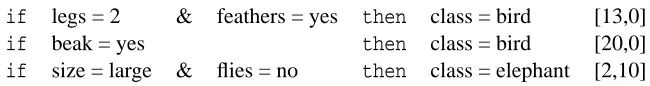
if legs = 2 & feathers = yes then class = bird [13,0]

if beak = yes then class = bird [20,0]

if size = large & flies = no then class = elephant [2,10]

Table 1: A rule set consisting of two rules for class ‘bird’ and one rule for class ‘elephant’.

In the case of unordered rule sets, the distribution of covered training examples among classes is attached to each rule. Rules of the form:

ifCondthenClass [ClassDistribution]

are induced, where numbers in the ClassDistribution list denote, for each individual class, how many training examples of this class are covered by the rule. When classifying a new example, all rules are tried and those covering the example are collected. If a clash occurs (several rules with different class predictions cover the example), a voting mechanism is used to obtain the final prediction: the class distributions attached to the rules are summed to determine the most probable class. If no rule fires, the default rule is invoked to predict the majority class of training instances not covered by the other rules in the list.

Probabilistic classification is illustrated on a sample classification task, taken from Clark and Boswell (1991). Suppose we need to classify an animal which is a two-legged, feathered, large, non-flying and has a beak,3, and the classification is based on a rule set, listed in Table 1 formed of three probabilistic rules with the [bird, elephant] class distribution assigned to each rule (for simplicity, the rule set does not include the default rule). All rules fire for the animal to be classified, resulting in a [35,10] class distribution. As a result, the animal is classified as a bird.

3. The CN2-SD Subgroup Discovery Algorithm

The main modifications of the CN2 algorithm, making it appropriate for subgroup discovery, involve the implementation of the weighted covering algorithm, incorporation of example weights into the weighted relative accuracy heuristic, probabilistic classification also in the case of the ‘ordered’ induction algorithm, and the area under ROC curve rule set evaluation. This section describes the CN2 modifications, while ROC analysis and a novel interpretation of the weighted relative accuracy heuristic in ROC space are given in Section 4.

3.1 Weighted Covering Algorithm

If used for subgroup discovery, one of the problems of standard rule learners, such as CN2 and RIPPER, is the use of the covering algorithm for rule set construction. The main deficiency of the covering algorithm is that only the first few induced rules may be of interest as subgroup descriptions with sufficient coverage and significance. In the subsequent iterations of the covering algorithm, rules are induced from biased example subsets, i.e., subsets including only positive examples that are not covered by previously induced rules, which inappropriately biases the subgroup discovery process.

(7)

As a remedy to this problem we propose the use of a weighted covering algorithm (Gamberger and Lavraˇc, 2002), in which the subsequently induced rules (i.e., rules induced in the later stages) also represent interesting and sufficiently large subgroups of the population. The weighted covering algorithm modifies the classical covering algorithm in such a way that covered positive examples are not deleted from the current training set. Instead, in each run of the covering loop, the algorithm stores with each example a count indicating how often (with how many rules) the example has been covered so far. Weights derived from these example counts then appear in the computation of WRAcc. Initial weights of all positive examples ejequal 1, w(ej,0) =1. The initial example weight

w(ej,0) =1 means that the example has not been covered by any rule, meaning ‘please cover this

example, since it has not been covered before’, while lower weights, 0<w<1 mean ‘do not try too hard on this example’. Consequently, the examples already covered by one or more constructed rules decrease their weights while the uncovered target class examples whose weights have not been decreased will have a greater chance to be covered in the following iterations of the algorithm.

For a weighted covering algorithm to be used, we have to specify the weighting scheme, i.e., how the weight of each example decreases with the increasing number of covering rules. We have implemented two weighting schemes described below.

3.1.1 MULTIPLICATIVEWEIGHTS

In the first scheme, weights decrease multiplicatively. For a given parameter 0<γ<1, weights of covered positive examples decrease as follows: w(ej,i) =γi, where w(ej,i)is the weight of example

ej being covered by i rules. Note that the weighted covering algorithm withγ=1 would result in

finding the same rule over and over again, whereas with γ=0 the algorithm would perform the same as the standard CN2 covering algorithm.

3.1.2 ADDITIVEWEIGHTS

In the second scheme, weights of covered positive examples decrease according to the formula w(ej,i) =_i+11 . In the first iteration all target class examples contribute the same weight w(ej,0) =1,

while in the following iterations the contributions of examples are inversely proportional to their coverage by previously induced rules.

3.2 Modified WRAcc Heuristic with Example Weights

The modification of CN2 reported in the work of Todorovski et al. (2000) affected only the heuristic function: weighted relative accuracy was used as a search heuristic, instead of the accuracy heuristic of the original CN2, while everything else remained the same. In this work, the heuristic function is further modified to handle example weights, which provide the means to consider different parts of the example space in each iteration of the weighted covering algorithm.

In the WRAcc computation (Equation 1) all probabilities are computed by relative frequencies. An example weight measures how important it is to cover this example in the next iteration. The modified WRAcc measure is then defined as follows:

WRAcc(Class_←Cond) =n0(Cond) N0 ·(

n0(Class.Cond) n0₍_Cond₎ −

(8)

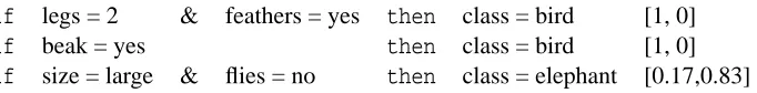
if legs = 2 & feathers = yes then class = bird [1, 0]

if beak = yes then class = bird [1, 0]

if size = large & flies = no then class = elephant [0.17,0.83]

Table 2: The rule set of Table 1 as treated by CN2-SD.

In this equation, N0 is the sum of the weights of all examples, n0(Cond)is the sum of the weights of all covered examples, and n0(Class.Cond) is the sum of the weights of all correctly covered examples.

To add a rule to the generated rule set, the rule with the maximum WRAcc measure is chosen out of those rules in the search space, which are not yet present in the rule set produced so far (all rules in the final rule set are thus distinct, without duplicates).

3.3 Probabilistic Classification

Each CN2 rule returns a class distribution in terms of the number of examples covered, as distributed over classes. The CN2 algorithm uses class distribution in classifying unseen instances only in the case of unordered rule sets, where rules are induced separately for each class. In the case of ordered decision lists, the first rule that fires provides the classification. In our modified CN2-SD algorithm, also in the ordered case all applicable rules are taken into account, hence probabilistic classification is used in both classifiers. This means that the terminology ‘ordered’ and ‘unordered’, which in CN2 distinguished between decision list and rule set induction, has a different meaning in our setting: the ‘unordered’ algorithm refers to learning classes one by one, while the ‘ordered’ algorithm refers to finding best rule conditions and assigning the majority class in the rule head.

Note that CN2-SD does not use the same probabilistic classification scheme as CN2. Unlike CN2, where the rule class distribution is computed in terms of the numbers of examples covered, CN2-SD treats the class distribution in terms of probabilities (computed by the relative frequency estimate). Table 2 presents the three rules of Table 1 with the class distribution expressed with probabilities. A two-legged, feathered, large, non-flying animal with a beak is again classified as a bird but now the probabilities are averaged (instead of summing the numbers of examples), resulting in the final probability distribution [0.72,0.28]. By using this voting scheme the subgroups covering a small number of examples are not so heavily penalized (as is the case in CN2) when classifying a new example.

3.4 CN2-SD Implementation

(9)

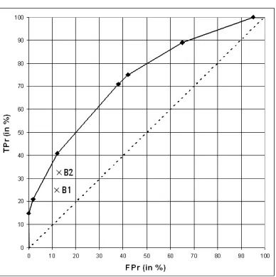
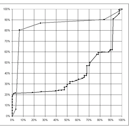
Figure 1: The ROC space with T Pr on the X axis and FPr on the Y axis. The solid line connecting seven optimal subgroups (marked by ) is the ROC convex hull. B1 and B2 denote suboptimal subgroups (marked by x). The dotted line – the diagonal connecting points (0,0) and (100,100) – indicates positions of insignificant rules with zero relative accuracy.

4. ROC Analysis for Subgroup Discovery

In this section we describe how ROC (Receiver Operating Characteristic) analysis (Provost and Fawcett, 2001) can be used to understand subgroup discovery and to visualize and evaluate discov-ered subgroups.

A point in ROC space shows classifier performance in terms of false alarm or false positive rate FPr= FP

T N+FP (plotted on the X -axis), and sensitivity or true positive rate T Pr= T P+FNT P (plotted

on the Y -axis). In terms of the expressions introduced in Sections 2.1 and 2.2, T P (true positives), FP (false positives), T N (true negatives) and FN (false negatives) can be expressed as: T P= n(Class.Cond), FP=n(Class.Cond), T N=n(Class.Cond)and FN=n(Class.Cond), where Class and Cond stand for_¬Class and_¬Cond, respectively.

(10)

4.1 The Interpretation of Weighted Relative Accuracy in ROC Space

Weighted relative accuracy is appropriate for measuring the quality of a single subgroup, because it is proportional to the distance from the diagonal in ROC space.4To see that this holds, note first that rule accuracy p(Class_|Cond)is proportional to the angle between the X -axis and the line connecting the origin with the point depicting the rule in terms of its T Pr/FPr tradeoff in ROC space. So, for instance, the X -axis has always rule accuracy 0 (these are purely negative subgroups), the Y -axis has always rule accuracy 1 (purely positive subgroups), and the diagonal represents subgroups with rule accuracy p(Class), the prior probability of the positive class. Consequently, all point on the diagonal represent insignificant subgroups.

Relative accuracy, p(Class_|Cond)₋p(Class), re-normalizes this such that all points on the diagonal have relative accuracy 0, all points on the Y -axis have relative accuracy 1₋p(Class) = p(Class) (the prior probability of the negative class), and all points on the X -axis have relative accuracy ₋p(Class). Notice that all points on the diagonal also have WRAcc=0. In terms of subgroup discovery, the diagonal represents all subgroups with the same target distribution as the whole population; only the generality of these ‘average’ subgroups increases when moving from left to right along the diagonal. This interpretation is slightly different in classifier learning, where the diagonal represents random classifiers that can be constructed without any training.

More generally, WRAcc isometrics lie on straight lines parallel to the diagonal (Flach, 2003, F¨urnkranz and Flach, 2003). Consequently, a point on the line T Pr=FPr+a, where a is the vertical distance of the line to the diagonal, has WRAcc=a.p(Class)p(Class). Thus, given a fixed class distribution, WRAcc is proportional to the vertical distance a to the diagonal. In fact, the quantity T Pr₋FPr would be an alternative quality measure for subgroups, with the additional advantage that it allows for comparison of subgroups from populations with different class distributions.

4.2 Methods for Constructing ROC Curves and AUC Evaluation

Subgroups obtained by CN2-SD can be evaluated in ROC space in two different ways.

4.2.1 AUC-METHOD-1

The first method treats each rule as a separate subgroup which is plotted in ROC space in terms of its true and false positive rates (T Pr and FPr). We then generate the convex hull of this set of points, selecting the subgroups which perform optimally under a particular range of operating characteristics. The area under this ROC convex hull (AUC) indicates the combined quality of the optimal subgroups, in the sense that it does evaluate whether a particular subgroup has anything to add in the context of all the other subgroups. However, this method does not take account of any overlap between subgroups, and subgroups not on the convex hull are simply ignored.

Figure 2 presents two ROC curves, showing the performance of CN2 and CN2-SD algorithms on the Australian UCI data set.

4.2.2 AUC-METHOD-2

The second method employs the combined probabilistic classifications of all subgroups, as indi-cated below. If we always choose the most likely predicted class, this corresponds to setting a fixed threshold 0.5 on the positive probability (the probability of the target class): if the positive

(11)

Figure 2: Example ROC curves (AUC-Method-1) on the Australian UCI data set: the solid curve for the standard CN2 classification rule learner, and the dotted curve for CN2-SD.

ity is larger than this threshold we predict positive, else negative. The ROC curve can be constructed by varying this threshold from 1 (all predictions negative, corresponding to (0,0) in ROC space) to 0 (all predictions positive, corresponding to (1,1) in ROC space). This results in n+1 points in ROC space, where n is the total number of classified examples (test instances). Equivalently, we can order all the classified examples by decreasing predicted probability of being positive, and tracing the ROC curve by starting in (0,0), stepping up when the example is actually positive and stepping to the right when it is negative, until we reach (1,1).5 Each point on this curve corresponds to a classifier defined by a possible probability threshold, as opposed to AUC-Method-1, where a point on the ROC curve corresponds to one of the optimal subgroups. The ROC curve depicts a set of classifiers, whereas the area under this ROC curve indicates the combined quality of all subgroups (i.e., the quality of the entire rule set). This method can be used with a test set or in cross-validation, but the resulting curve is not necessarily convex.6

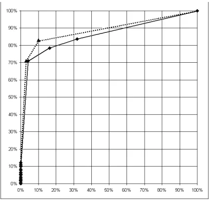
Figure 3 presents two ROC curves, showing the performance of the CN2 and CN2-SD algo-rithms on the Australian UCI data set. It is apparent from this figure that CN2 is badly overfitting on this data set, because almost all of its ROC curve is below the diagonal. This is because CN2 has learned many overly specific rules, which bias the predicted probabilities. These overly specific rules are visible in Figure 2 as points close to the origin.

5. In the case of ties, we make the appropriate number of steps up and to the right at once, drawing a diagonal line segment.

(12)

Figure 3: Example ROC curves (AUC-Method-2) on the Australian UCI data set: the solid curve for the standard CN2 classification rule learner, and the dotted curve for CN2-SD.

4.2.3 COMPARISON OF THETWOAUC METHODS

Which of the two methods is more appropriate for subgroup discovery is open for debate. The second method seems more appropriate if the discovered subgroups are intended to be applied also in the predictive setting, as a rule set (a model) used for classification. Its advantage is also that it is easier to apply cross-validation. In the experimental evaluation in Section 6 we use AUC-Method-2 in the comparison of the predictive performance of rule learners.

An argument in favor of using AUC-Method-1 for subgroup evaluation is based on the obser-vation that AUC-Method-1 suggests to eliminate, from the induced set of subgroup descriptions, those rules which are not on the ROC convex hull. This seems appropriate, as the ‘best’ subgroups according to the WRAcc evaluation measure, are subgroups most distant from the ROC diagonal. However, disjoint subgroups, either on or close to the convex hull, should not be eliminated, as (due to disjoint coverage and possibly different symbolic descriptions) they may represent interesting subgroups, regardless of the fact that there is another ‘better’ subgroup on the ROC convex hull, with a similar T Pr/FPr tradeoff.

Notice that the area under ROC curve (AUC-Method-1) cannot be used as a predictive qual-ity measure when comparing different subgroup miners, because it does not take into account the overlapping structure of subgroups. An argument against the use of this measure is here elaborated through a simple example.7Consider for instance two subgroup mining results, of say 3 subgroups in each resulting rule set. The first result set consists of three disjoint subgroups of equal size that together cover all the examples of the selected Class value and have a 100% accuracy. Thus these three subgroups are a perfect classifier for the Class value. In ROC space the three subgroups collapse at the point (0,1/3). The second result set consists of three equal subgroups (having a

(13)

imum overlap: with different descriptions, but equal extensions), also with a 100% accuracy and covering one third of the class examples. Clearly the first result is better, but the representation of the results in ROC space (and the area under ROC curve) is the same for both cases.

5. Subgroup Evaluation Measures

In this section we distinguish between predictive and descriptive evaluation measures, which is in-line with the distinction of predictive induction and descriptive induction made in Section 1. Descriptive measures are used to evaluate the quality of individual rules (individual patterns). These quality measures are the most appropriate for subgroup discovery, as the task of subgroup discovery is to induce individual patterns of interest. Predictive measures are used in addition to descriptive measures just to show that the CN2-SD subgroup discovery mechanisms perform well also in the predictive induction setting, where the goal is to induce a classifier.

5.1 Descriptive Measures of Rule Interestingness

Descriptive measures of rule interestingness evaluate each individual subgroup and are thus appro-priate for evaluating the success of subgroup discovery. The proposed quality measures compute the average over the induced set of subgroup descriptions, which enables the comparison between different algorithms.

Coverage. The average coverage measures the percentage of examples covered on average by one

rule of the induced rule set. Coverage of a single rule Riis defined as

Cov(Ri) =Cov(Class←Condi) =p(Condi) =

n(Condi)

N .

The average coverage of a rule set is computed as

COV = 1 nR

nR

∑

i=1

Cov(Ri),

where nRis the number of induced rules.

Support. For subgroup discovery it is interesting to compute the overall support (the target

cover-age) as the percentage of target examples (positives) covered by the rules, computed as the true positive rate for the union of subgroups. Support of a rule is defined as the frequency of correctly classified covered examples:

Sup(Ri) =Sup(Class←Condi) =p(Class.Condi) =

n(Class.Condi)

N .

The overall support of a rule set is computed as

SU P= 1 N_Class

∑

j

n(Classj· _

Classj←Condi

Condi),

(14)

Size. Size is a measure of complexity (the syntactical complexity of induced rules). The rule set

size is computed as the number of rules in the induced rule set (including the default rule):

SIZE=nR.

In addition to rule set size used in this paper, complexity could be measured also by the average number of rules/subgroups per class, and the average number of features per rule.

Significance. Average rule significance is computed in terms of the likelihood ratio of a rule,

nor-malized with the likelihood ratio of the significance threshold (99%); the average is computed over all the rules. Significance (or evidence, in the terminology of Kl¨osgen, 1996) indicates how significant is a finding, if measured by this statistical criterion. In the CN2 algorithm (Clark and Niblett, 1989), significance is measured in terms of the likelihood ratio statistic of a rule as follows:

Sig(Ri) =Sig(Class←Condi) =2·

∑

j

n(Classj.Condi)·log

n(Classj.Condi)

n(Classj)·p(Condi)

(2)

where for each class Classj, n(Classj.Condi)denotes the number of instances of Classjin the

set where the rule body holds true, n(Classj)is the number of Classjinstances, and p(Condi)

(i.e., rule coverage computed as n(Condi)

N ) plays the role of a normalizing factor. Note that

although for each generated subgroup description one class is selected as the target class, the significance criterion measures the distributional unusualness unbiased to any particular class – as such, it measures the significance of rule condition only.

The average significance of a rule set is computed as:

SIG= 1 nR

nR

∑

i=1

Sig(Ri).

Unusualness. Average rule unusualness is computed as the average WRAcc computed over all the

rules:

W RACC= 1 nR

nR

∑

i=1

WRAcc(Ri).

As discussed in Section 4.1, WRAcc is appropriate for measuring the unusualness of separate subgroups, because it is proportional to the vertical distance from the diagonal in the ROC space (see the underlying reasoning in Section 4.1).

As WRAcc is proportional to the distance to the diagonal in ROC space, WRAcc also reflects rule significance – the larger WRAcc, the more significant the rule, and vice versa. As both WRAcc and rule significance measure the distributional unusualness of a subgroup, they are the most important quality measures for subgroup discovery. However, while significance only measures distributional unusualness, WRAcc takes also rule coverage into account, therefore we consider unusualness – computed by the average WRAcc – to be the most appropriate measure for subgroup quality evalu-ation.

(15)

5.2 Predictive Measures of Rule Set Classification Performance

Predictive measures evaluate a rule set, interpreting a set of subgroup descriptions as a predictive model. Despite the fact that optimizing accuracy is not the intended goal of subgroup discovery algorithms, these measures can be used in order to provide a comparison of CN2-SD with standard classification rule learners.

Predictive accuracy. The percentage of correctly predicted instances. For a binary classification

problem, rule set accuracy is computed as follows:

ACC= T P+T N T P+T N+FP+FN.

Note that ACC measures the accuracy of the whole rule set on both positive and negative examples, while rule accuracy (defined as Acc(Class←Cond) = p(Class|Cond)) measures the accuracy of a single rule on positives only.

Area under ROC curve. The AUC-Method-2, described in Section 4.2, applicable to rule sets is

selected as the evaluation measure. It interprets a rule set as a probabilistic model, given all the different probability thresholds as defined through the probabilistic classification of test instances.

6. Experimental Evaluation

For subgroup discovery, expert evaluation of results is of ultimate interest. Nevertheless, before applying the proposed approach to a particular problem of interest, we wanted to verify our claims that the mechanisms implemented in the CN2-SD algorithm are indeed appropriate for subgroup discovery. For this purpose we tested it on selected UCI data sets. In this paper we use the same data sets as in the work of Todorovski et al. (2000). We have applied CN2-SD also to a real life problem of traffic accident analysis; these results were evaluated also by the expert.

6.1 The Experimental Setting

To test the applicability of CN2-SD to the subgroup discovery task, we compare its performance with the performance of the standard CN2 classification rule learning algorithm (referred to as CN2-standard, and described in the work of Clark and Boswell, 1991) as well as with the CN2 algorithm using WRAcc (CN2-WRAcc, described by Todorovski et al., 2000).

In this comparative study all the parameters of the CN2 algorithm are set to their default values (beam-size = 5, significance-threshold = 99%). The results of the CN2-SD algorithm are computed using both multiplicative weights (withγ= 0.5, 0.7, 0.9)8and additive weights.

We estimate the performance of the algorithms using stratified 10-fold cross-validation. The obtained estimates are presented in terms of their average values and standard deviations.

Statistical significance of the difference in performance compared to CN2-standard is tested using the paired t-test (exactly the same folds are used in all comparisons) with significance level of 95%: bold font and↑to the right of a result in all the tables means that the algorithm is significantly better than CN2-standard while_↓means it is significantly worse. The same paired t-test is used to compare the different versions of our algorithm with CN2-standard over all the data sets.

(16)

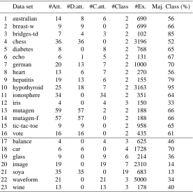
Data set #Att. #D.att. #C.att. #Class #Ex. Maj. Class (%)

1 australian 14 8 6 2 690 56

2 breast-w 9 9 0 2 699 66

3 bridges-td 7 4 3 2 102 85

4 chess 36 36 0 2 3196 52

5 diabetes 8 0 8 2 768 65

6 echo 6 1 5 2 131 67

7 german 20 13 7 2 1000 70

8 heart 13 6 7 2 270 56

9 hepatitis 19 13 6 2 155 79

10 hypothyroid 25 18 7 2 3163 95

11 ionosphere 34 0 34 2 351 64

12 iris 4 0 4 3 150 33

13 mutagen 59 57 2 2 188 66

14 mutagen-f 57 57 0 2 188 66

15 tic-tac-toe 9 9 0 2 958 65

16 vote 16 16 0 2 435 61

17 balance 4 0 4 3 625 46

18 car 6 6 0 4 1728 70

19 glass 9 0 9 6 214 36

20 image 19 0 19 7 2310 14

21 soya 35 35 0 19 683 13

22 waveform 21 0 21 3 5000 34

23 wine 13 0 13 3 178 40

Table 3: Properties of the UCI data sets.

6.2 Experiments on UCI Data Sets

We experimentally evaluate our approach on 23 data sets from the UCI Repository of Machine Learning Databases (Murphy and Aha, 1994). Table 3 gives an overview of the selected data sets in terms of the number of attributes (total, discrete, continuous), the number of classes, the number of examples, and the percentage of examples of the majority class. These data sets have been widely used in other comparative studies (Todorovski et al., 2000). We have divided the data sets in two groups (Table 3), those with two classes (binary data sets 1–16) and those with more then two classes (multi-class data sets 17–23). This distinction is made as ROC analysis is applied only on binary data sets.9

6.2.1 RESULTS OF THEUNORDEREDCN2-SD

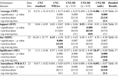
Tables 4 and 5 present summary results of the UCI experiments, while details can be found in Ta-bles 14–20 in Appendix A. For each performance measure, the summary table shows the average value over all the data sets, the significance of the results compared to CN2-standard (p-value), win/loss/draw in terms of the number of data sets in which the results are better/worse/equal com-pared with CN2-standard, as well as the number of significant wins and losses.

(17)

Performance Data CN2 CN2 CN2-SD CN2-SD CN2-SD Detailed

Measure Sets standard WRAcc (γ=0.5) (γ=0.9) (add.) Results

Coverage (COV) 23 0.131±0.14 0.311±0.17 0.403±0.23 0.450±0.26 0.486±0.30 Table 14

•significance – p value 0.000 0.000 0.000 0.000

•win/loss/draw 22/1/0 22/1/0 23/0/0 22/1/0

•sig.win/sig.loss 21/1 22/0 22/0 21/1

Support (SUP) 23 0.84±0.03 0.85±0.03 0.90±0.06 0.92±0.06 0.91±0.06 Table 15

•significance – p value 0.637 0.000 0.000 0.001

•win/loss/draw 13/10/0 18/5/0 20/3/0 16/7/0

•sig.win/sig.loss 5/4 13/1 18/0 13/1

Size (SIZE) 23 18.18±21.77 6.15±4.49 6.25±4.42 6.49±4.57 6.35±4.58 Table 16

•significance – p value 0.006 0.007 0.007 0.007

•win/loss/draw 22/1/0 22/1/0 20/3/0 23/0/0

•sig.win/sig.loss 22/0 21/0 19/2 18/0

Significance (SIG) 23 2.11±0.46 8.97±4.66 15.57±6.05 16.92±8.90 18.47±9.00 Table 17

•win/loss/draw 22/1/0 23/0/0 22/1/0 23/0/0

•sig.win/sig.loss 21/0 23/0 21/0 23/0

Unusualness (WRACC) 23 0.017±0.02 0.056±0.05 0.079±0.06 0.088±0.06 0.092±0.07 Table 18

•win/loss/draw 20/1/2 22/1/0 22/1/0 22/1/0

•sig.win/sig.loss 19/1 21/1 21/1 21/1

Table 4: Summary of the experimental results on the UCI data sets (descriptive evaluation mea-sures) for different variants of the unordered algorithm using 10-fold stratified cross-validation. The best results are shown in boldface.

The analysis shows that if multiplicative weights are used, most results improve with the in-creased value of the γparameter. As in most cases the best CN2-SD variants are CN2-SD with

γ=0.9 and with additive weights, and as using additive weighs is the simpler method, the additive weights setting is recommended as default for experimental use.

The summary of results in terms of descriptive measures of interestingness is as follows.

• In terms of the average coverage per rule CN2-SD produces rules with significantly higher coverage (the higher the coverage the better the rule) than both CN2-WRAcc and CN2-standard. The coverage is increased by increasing theγparameter and the best results are achieved by

γ=0.9 and by additive weights.

• CN2-SD induces rule sets with significantly larger overall support than CN2-standard mean-ing that it covers a higher percentage of target examples (positives) thus leavmean-ing a smaller number of examples unclassified.10

• CN2-WRAcc and CN2-SD induce rule sets that are significantly smaller than CN2-standard (smaller rule sets are better), while rule sets of CN2-WRAcc and CN2-SD are comparable, de-spite the fact that CN2-SD uses weights to ‘recycle’ examples and thus produces overlapping rules.

(18)

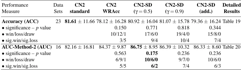
Performance Data CN2 CN2 CN2-SD CN2-SD CN2-SD Detailed

Measure Sets standard WRAcc (γ=0.5) (γ=0.9) (add.) Results

Accuracy (ACC) 23 81.61±11.66 78.12±16.28 80.92±16.04 81.07±15.78 79.36±16.24 Table 19

•significance – p value 0.150 0.771 0.818 0.344

•win/loss/draw 10/12/1 17/6/0 19/4/0 15/8/0

•sig.win/sig.loss 3/5 9/4 10/4 7/4

AUC-Method-2 (AUC) 16 82.16±16.81 84.37±9.87 86.75±8.95 86.39±10.32 86.33±8.60 Table 20

•significance – p value 0.563 0.175 0.236 0.236

•win/loss/draw 6/9/1 10/6/0 9/7/0 10/6/0

•sig.win/sig.loss 5/5 6/2 7/4 6/3

Table 5: Summary of the experimental results on the UCI data sets (predictive evaluation measures) for different variants of the unordered algorithm using 10-fold stratified cross-validation. The best results are shown in boldface.

• CN2-SD induces significantly better rules in terms of rule significance (rules with higher significance are better) computed by the average likelihood ratio: while the ratios achieved by CN2-standard are already significant at the 99% level, this is further pushed up by CN2-SD with maximum values achieved by additive weights. An interesting question, to be verified in further experiments, is whether the weighted versions of the CN2 algorithm improve the significance of the induced subgroups also in the case when CN2 rules are induced without applying the significance test.

• In terms of rule unusualness which is of ultimate interest to the subgroup discovery task, CN2-SD produces rules with significantly higher average weighted relative accuracy than CN2-standard. Like in the case of average coverage per rule the unusualness is increased by increasing theγ parameter and the best results are achieved byγ=0.9 and by additive weights. Note that the unusualness of a rule, computed by its WRAcc, is a combination of rule accuracy, coverage and prior probability of the target class.

In terms of predictive measures of classification performance results can be summarized as follows.

• CN2-SD improves the accuracy in comparison with CN2-WRAcc and performs compara-ble to CN2-standard (the difference is insignificant). Notice however that while optimiz-ing predictive accuracy is the ultimate goal of CN2, for CN2-SD the goal is to optimize the coverage/relative-accuracy tradeoff.

• In the computation of area under ROC curve (AUC-Method-2) due to the restriction of this method to binary class data sets, only 16 binary data sets are used in the comparisons. Notice that CN2-SD improves the area under ROC curve compared to CN2-WRAcc and compared to CN2-standard, but the differences are not significant. The area under ROC curve however seems not to be affected by the parameterγor by the weighting approach of CN2-SD.

(19)

6.2.2 RESULTS OF THEORDEREDCN2-SD

For completeness, the results for different versions of the ordered algorithm are summarized in Tables 6 and 7, without giving the results for individual data sets in Appendix A. In our view, the unordered CN2-SD algorithm is more appropriate for subgroup discovery than the ordered variant, as it induces a set of rules for each target class in turn.

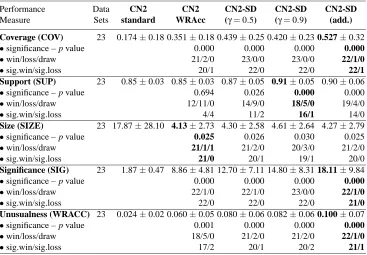
Performance Data CN2 CN2 CN2-SD CN2-SD CN2-SD

Measure Sets standard WRAcc (γ=0.5) (γ=0.9) (add.)

Coverage (COV) 23 0.174±0.18 0.351±0.18 0.439±0.25 0.420±0.23 0.527±0.32

•win/loss/draw 21/2/0 23/0/0 23/0/0 22/1/0

•sig.win/sig.loss 20/1 22/0 22/0 22/1

Support (SUP) 23 0.85±0.03 0.85±0.03 0.87±0.05 0.91±0.05 0.90±0.06

•win/loss/draw 12/11/0 14/9/0 18/5/0 19/4/0

•sig.win/sig.loss 4/4 11/2 16/1 14/0

Size (SIZE) 23 17.87±28.10 4.13±2.73 4.30±2.58 4.61±2.64 4.27±2.79

•significance – p value 0.025 0.026 0.030 0.025

•win/loss/draw 21/1/1 21/2/0 20/3/0 21/2/0

•sig.win/sig.loss 21/0 20/1 19/1 20/0

Significance (SIG) 23 1.87±0.47 8.86±4.81 12.70±7.11 14.80±8.31 18.11±9.84

•win/loss/draw 22/1/0 22/1/0 23/0/0 22/1/0

•sig.win/sig.loss 22/0 22/0 22/0 21/0

Unusualness (WRACC) 23 0.024_±0.02 0.060_±0.05 0.080_±0.06 0.082_±0.06 0.100_±0.07

•win/loss/draw 18/5/0 21/2/0 21/2/0 22/1/0

•sig.win/sig.loss 17/2 20/1 20/2 21/1

Table 6: Summary of the experimental results on the UCI data sets (descriptive evaluation mea-sures) for different variants of the ordered algorithm using 10-fold stratified cross-validation. The best results are shown in boldface.

6.3 Experiments in Traffic Accident Data Analysis

We have evaluated the CN2-SD algorithm also on a traffic accident data set. This is a large real-world database (1.5 GB) containing 21 years of police traffic accident reports (1979–1999). The analysis of this database is not straightforward because of the volume of the data, the amounts of noise and missing data, and the fact that there is no clearly defined data mining target. As described below, some preprocessing was needed before running the subgroup discovery experiments. Results of experiments were shown to the domain expert whose comments are included.

6.3.1 THETRAFFICACCIDENTDATASET

(20)

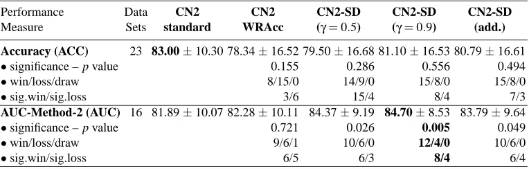
Performance Data CN2 CN2 CN2-SD CN2-SD CN2-SD

Measure Sets standard WRAcc (γ=0.5) (γ=0.9) (add.)

Accuracy (ACC) 23 83.00±10.30 78.34±16.52 79.50±16.68 81.10±16.53 80.79±16.61

•significance – p value 0.155 0.286 0.556 0.494

•win/loss/draw 8/15/0 14/9/0 15/8/0 15/8/0

•sig.win/sig.loss 3/6 15/4 8/4 7/3

AUC-Method-2 (AUC) 16 81.89±10.07 82.28±10.11 84.37±9.19 84.70±8.53 83.79±9.64

•win/loss/draw 9/6/1 10/6/0 12/4/0 10/6/0

•sig.win/sig.loss 6/5 6/3 8/4 6/4

Table 7: Summary of the experimental results on the UCI data sets (predictive evaluation measures) for different variants of the ordered algorithm using 10-fold stratified cross-validation. The best results are shown in boldface.

happened over the given period of time (1979–1999), the VEHICLE table contains data about the vehicles involved in those accidents, and the CASUALTY table contains data about the casualties involved in the accidents. Consider the following example: “Two vehicles crashed in a traffic accident and three people were seriously injured in the crash”. In terms of the traffic data set this is recorded as one record in the ACCIDENT table, two records in the VEHICLE table and three records in the CASUALTY table. The three tables are described in more detail below.

• The ACCIDENT table contains one record for each accident. The 30 attributes describing an accident can be divided in three groups: date and time of the accident, description of the road where the accident has occurred, and conditions under which the accident has occurred (such as weather conditions, light and junction details). In the ACCIDENT table there are more than 5 million records.

• The VEHICLE table contains one record for each vehicle involved in an accident from the ACCIDENT table. There can be one or many vehicles involved in a single accident. The VEHICLE table attributes describe the type of the vehicle, maneuver and direction of the vehicle (from and to), vehicle location on the road, junction location at impact, sex and age of the driver, alcohol test results, damage resulting from the accident, and the object that vehicle hit on and off carriageway. There are 24 attributes in the VEHICLE table which contains almost 9 million records.

• The CASUALTY table contains records about casualties for each of the vehicles in the VEHI-CLE table. There can be one or more casualties per vehicle. The CASUALTY table contains 16 attributes describing sex and age of casualty, type of casualty (e.g., pedestrian, cyclist, car occupant etc.), severity of casualty, if casualty type is pedestrian, what were his/her charac-teristics (location, movement, direction). This table contains almost 7 million records.

6.3.2 DATAPREPROCESSING

(21)

Number of Percentage of Class distribution (%)

PFC Examples Sampled Accidents fatal / serious / slight

1 2555 0.3 1.76 / 24.85 / 73.39

2 2523 1.9 2.53 / 30.87 / 66.60

3 2501 4.8 0.56 / 12.35 / 87.09

4 2499 1.9 2.16 / 27.21 / 70.63

5 2522 9.2 1.90 / 23.39 / 74.71

6 2548 2.0 1.41 / 13.69 / 84.90

7 2788 1.4 0.97 / 16.25 / 82.78

Table 8: Properties of the traffic data set.

the experiments on these samples. We focused on the ACCIDENT table and examined only the accidents that happened in 7 districts (called Police Force Codes, or PFCs) across the UK.11 The 7 PFCs were chosen by the domain expert and represent typical PFCs from clusters of PFCs with the same accident dynamics, analyzed by Ljubiˇc et al. (2002). In this way we obtained 7 data sets (one for each PFC) with some hundred thousands of examples each. We further sampled this data to obtain approximately 2500 examples per data set. The sample percentages are listed in Table 8 together with the other characteristics of these 7 sampled data sets.

Among the 26 attributes describing each of the 7 data sets we chose the attribute ‘accident severity’ to be the class attribute. The task that we have addressed was therefore to find subgroups of accidents of a certain severity (‘slight’, ‘serious’ or ‘fatal’) and characterize them in terms of attributes describing the accident, such as: ‘road class’, ‘speed limit’, ‘light condition’, etc.

6.3.3 RESULTS OFEXPERIMENTS

We want to investigate if by running CN2-SD on the data sets, described in Table 8, we are able to get some rules that are typical and different for distinct PFCs.

We used the same methodology to perform the experiments as in the case of the UCI data sets of Section 6.2. The only difference is that here we do not perform the area under ROC curve analysis, because the data sets are not two-class. The results presented in Tables 9–13 show the same advan-tages of CN2-SD over CN2-WRAcc and CN2-standard as shown by the results of experiments on the UCI data sets.12 In particular, CN2-SD produces substantially smaller rule sets, where individual rules have higher coverage and significance.

It should be noticed that these data sets have a very unbalanced class distribution (most accidents are ‘slight’ and only few are ‘fatal’, see Table 8). In terms of rule set accuracy, all algorithms achieved roughly default performance which is obtained by always predicting the majority class. Since classification was not the main interest of this experiment, we omit the results.

11. For the sake of anonymity, the code numbers 1 through 7 do not correspond to the PFCs 1 through 7 used for Police Force Codes in the actual traffic accident database.

(22)

CN2 CN2 CN2-SD CN2-SD CN2-SD CN2-SD

# standard WRAcc (γ=0.5) (γ=0.7) (γ=0.9) (add.)

COV±sd COV±sd COV±sd COV±sd COV±sd COV±sd

1 0.056±0.01 0.108↑ ±0.00 0.111↑ ±0.03 0.111↑ ±0.03 0.123↑ ±0.03 0.110↑ ±0.03

2 0.050±0.10 0.113↑ ±0.04 0.127↑ ±0.05 0.127↑ ±0.04 0.129↑ ±0.05 0.151↑ ±0.04

3 0.140±0.03 0.118±0.03 0.126±0.02 0.119±0.02 0.118±0.01 0.154±0.02

4 0.052±0.01 0.105↑ ±0.03 0.105↑ ±0.04 0.120↑ ±0.04 0.122↑ ±0.04 0.116↑ ±0.04

5 0.075±0.08 0.108↑ ±0.04 0.115↑ ±0.06 0.121↑ ±0.05 0.110↑ ±0.05 0.127↑ ±0.04

6 0.078±0.06 0.118↑ ±0.03 0.134↑ ±0.05 0.122↑ ±0.06 0.124↑ ±0.06 0.120↑ ±0.05

7 0.116±0.08 0.110±0.11 0.118±0.14 0.124±0.13 0.122±0.13 0.143↑ ±0.12

Average 0.081±0.03 0.111±0.01 0.120±0.01 0.121±0.00 0.121±0.01 0.132±0.02

•significance – p value 0.047 0.021 0.023 0.029 0.003

•win/loss/draw 5/2/0 6/1/0 6/1/0 6/1/0 7/0/0

•sig.win/sig.loss 5/0 5/0 5/0 5/0 6/0

Table 9: Experimental results on the traffic accident data sets. Average coverage per rule with standard deviation (COV_±sd) for different variants of the unordered algorithm.

SUP±sd SUP±sd SUP±sd SUP±sd SUP±sd SUP±sd

1 0.86±0.03 0.89±0.02 0.83±0.06 0.93↑ ±0.04 0.96↑ ±0.02 0.95↑ ±0.03

2 0.84±0.02 0.85±0.09 0.85±0.02 0.92↑ ±0.04 0.93↑ ±0.00 0.84±0.08

3 0.81±0.06 0.82±0.04 0.93↑ ±0.02 0.90↑ ±0.05 0.97↑ ±0.01 0.85±0.06

4 0.80±0.04 0.87↑ ±0.05 0.82±0.05 0.83±0.00 0.91↑ ±0.03 0.81±0.10

5 0.87_±0.08 0.85_±0.03 0.80_{↓ ±}0.03 0.83_±0.06 0.94_{↑ ±}0.02 0.83_±0.08

6 0.84±0.06 0.88↑ ±0.07 0.81±0.09 0.91↑ ±0.06 0.88↑ ±0.07 0.98↑ ±0.01

7 0.81±0.08 0.83±0.05 0.90↑ ±0.01 0.81±0.01 0.95↑ ±0.02 0.99↑ ±0.00

Average 0.83±0.03 0.85±0.02 0.85±0.05 0.88±0.05 0.93±0.03 0.89±0.08

•significance – p value 0.056 0.548 0.053 0.001 0.092

•win/loss/draw 6/1/0 4/3/0 6/1/0 7/0/0 6/1/0

•sig.win/sig.loss 2/0 2/1 4/0 7/0 3/0

Table 10: Experimental results on the traffic accident data sets. Overall support of rule sets with standard deviation (SUP_±sd) for different variants of the unordered algorithm.

6.3.4 EVALUATION BY THEDOMAINEXPERT

We have further examined the rules induced by the CN2-SD algorithm (using additive weights). We focused on rules with high coverage and rules that cover a high percentage of the predicted class as these are the rules that are likely to reflect some regularity in the data.

(23)

SIZE±sd SIZE±sd SIZE±sd SIZE±sd SIZE±sd SIZE±sd

1 16.7±0.60 9.3↑ ±0.99 10.0↑ ±0.51 10.6↑ ±0.46 10.6↑ ±0.73 9.5↑ ±0.25

2 18.7±1.28 9.2↑ ±0.33 10.0↑ ±0.20 10.3↑ ±0.21 10.3↑ ±0.56 11.1↑ ±0.23

3 7.0±0.30 8.6±0.95 9.2±0.19 10.2↓ ±0.14 9.5±0.35 9.8↓ ±0.19

4 18.0±1.39 9.9↑ ±0.59 10.4↑ ±0.31 11.2↑ ±0.64 11.2↑ ±0.24 10.3↑ ±0.56

5 12.8±1.44 9.6↑ ±0.19 10.1↑ ±0.51 11.2±0.84 11.6±0.96 9.7↑ ±0.21

6 12.5±0.31 8.5↑ ±0.35 9.3↑ ±0.51 8.7↑ ±0.91 9.4↑ ±0.60 8.5↑ ±0.39

7 8.6±1.41 9.3±0.41 9.9±0.90 10.8↓ ±0.73 11.1↓ ±0.13 10.4±0.59

Average 13.47±4.57 9.20±0.50 9.84±0.44 10.42±0.86 10.53±0.84 9.90±0.80

•significance – p value 0.040 0.066 0.123 0.127 0.075

•win/loss/draw 5/2/0 5/2/0 5/2/0 5/2/0 5/2/0

•sig.win/sig.loss 5/0 5/0 4/2 4/1 5/1

Table 11: Experimental results on the traffic accident data sets. Sizes of rule sets with standard deviation (SIZE_±sd) for different variants of the unordered algorithm.

SIG±sd SIG±sd SIG±sd SIG±sd SIG±sd SIG±sd

1 1.9±0.82 7.0↑ ±0.31 8.7↑ ±0.41 9.7↑ ±0.59 9.4↑ ±0.30 9.6↑ ±0.45

2 1.9±0.34 6.2↑ ±0.25 9.9↑ ±0.26 9.8↑ ±0.20 9.5↑ ±0.81 9.8↑ ±0.36

3 1.3±0.27 6.6↑ ±0.61 8.4↑ ±0.52 9.2↑ ±0.54 11.5↑ ±0.75 9.3↑ ±0.17

4 1.6_±0.10 7.6_{↑ ±}0.14 8.5_{↑ ±}0.79 11.0_{↑ ±}0.84 9.4_{↑ ±}0.80 11.1_{↑ ±}0.24

5 1.6±0.75 6.0↑ ±0.23 10.6↑ ±0.70 9.6↑ ±0.76 12.5↑ ±0.43 9.1↑ ±0.74

6 1.5±0.87 8.5↑ ±0.41 8.3↑ ±0.54 9.8↑ ±0.24 9.9↑ ±0.51 12.5↑ ±0.35

7 1.7±0.49 6.8↑ ±0.75 8.7↑ ±0.20 9.9↑ ±0.63 9.2↑ ±0.73 9.7↑ ±0.40

Average 1.64±0.20 6.95±0.86 9.01±0.89 9.85±0.56 10.20±1.28 10.16±1.21

•significance – p value 0.000 0.000 0.000 0.000 0.000

•win/loss/draw 7/0/0 7/0/0 7/0/0 7/0/0 7/0/0

•sig.win/sig.loss 7/0 7/0 7/0 7/0 7/0

Table 12: Experimental results on the traffic accident data sets. Average significance per rule with standard deviation (SIG±sd) for different variants of the unordered algorithm.

involved would also increase with accident severity. Contrary to these expectations we found rules of the following two kinds:

• Rules that cover more than the average proportion of ‘fatal’ or ‘serious’ accidents when just one vehicle is involved in the accident. Examples of such rules are:

IF nv < 1.500 THEN sev = "1" [15 280 1024]13 IF nv < 1.500 THEN sev = "2" [22 252 890]

(24)

WRACC±sd WRACC±sd WRACC±sd WRACC±sd WRACC±sd WRACC±sd

1 0.013±0.02 0.025↑ ±0.05 0.025↑ ±0.10 0.026↑ ±0.02 0.028↑ ±0.03 0.025↑ ±0.09

2 0.009±0.07 0.018↑ ±0.05 0.021↑ ±0.00 0.021↑ ±0.04 0.021↑ ±0.02 0.025↑ ±0.04

3 0.052±0.01 0.043±0.00 0.046±0.07 0.043±0.03 0.043±0.05 0.056±0.02

4 0.010±0.09 0.021↑ ±0.06 0.021↑ ±0.05 0.024↑ ±0.09 0.024↑ ±0.00 0.023↑ ±0.07

5 0.019±0.04 0.026↑ ±0.06 0.027↑ ±0.07 0.029↑ ±0.08 0.027↑ ±0.01 0.030↑ ±0.07

6 0.027±0.03 0.041↑ ±0.06 0.047↑ ±0.05 0.042↑ ±0.05 0.043↑ ±0.07 0.042↑ ±0.07

7 0.038±0.03 0.035±0.01 0.038±0.04 0.040±0.00 0.039±0.08 0.046±0.04

Average 0.024±0.02 0.030±0.01 0.032±0.01 0.032±0.01 0.032±0.01 0.035±0.01

•significance – p value 0.096 0.042 0.041 0.048 0.000

•win/loss/draw 5/2/0 5/2/0 6/1/0 6/1/0 7/0/0

•sig.win/sig.loss 5/0 5/0 5/0 5/0 5/0

Table 13: Experimental results on the traffic accident data sets. Unusualness of rule sets with stan-dard deviation (WRACC_±sd) for different variants of the unordered algorithm.

• Rules that cover more than the average proportion of ‘slight’ accidents when two or more vehicles are involved and there are few casualties. An example of such a rule is:

IF nv > 1.500 AND nc < 2.500 THEN sev = "3" [8 140 1190]

Having shown the induced results to the domain expert, he pointed out the following aspects of data collection for the data in the ACCIDENT table.14

• The severity code in the ACCIDENT table relates to the most severe injury among those reported for that accident. Therefore a multiple vehicle accident with 1 fatal and 20 slight injuries would be classified as fatal as one fatality occurred, while each individual casualty injury severity is coded in the CASUALTY table.

• Some (slight) injuries may be unreported at the accident scene: if the policeman compiled/revised the report after the event, new casualty/injury details can be reported (injuries that came to light after the event or reported for reasons relating to injury/insurance claims). However, these changes are not reflected in the ACCIDENT table.

The findings revealed by the rules were surprising to the domain expert and need further investi-gation. The analysis shows that examining the ACCIDENT table is not sufficient and that further examination of the VEHICLE and CASUALTY tables is needed in further work.

7. Related Work

Other systems have addressed the task of subgroup discovery, the best known being EXPLORA (Kl¨osgen, 1996) and MIDOS (Wrobel, 1997, 2001). EXPLORA treats the learning task as a sin-gle relation problem, i.e., all the data are assumed to be available in one table (relation), whereas

(25)

MIDOS extends this task to multi-relational databases. Other approaches deal with multi-relational databases using propositionalisation and aggregate functions can be found in the work of Knobbe et al. (2001, 2002).

Another approach to finding symbolic descriptions of groups of instances is symbolic cluster-ing, which has been popular for many years (Michalski, 1980, Gowda and Diday, 1992). Moreover, learning of concept hierarchies also aims at discovering groups of instances, which can be induced in a supervised or unsupervised manner: decision tree induction algorithms perform supervised symbolic learning of concept hierarchies (Langley, 1996, Raedt and Blockeel, 1997), whereas hi-erarchical clustering algorithms (Sokal and Sneath, 1963, Gordon, 1982) are unsupervised and do not result in symbolic descriptions. Note that in decision tree learning, the rules which can be formed from paths leading from the root node to class labels in the leaves represent discriminant descriptions, formed from properties that best discriminate between the classes. As rules formed from decision tree paths form discriminant descriptions, they are inappropriate for solving subgroup discovery tasks which aim at describing subgroups by their characteristic properties.

Instance weights play an important role in boosting (Freund and Shapire, 1996) and alternating decision trees (Schapire and Singer, 1998). Instance weights have been used also in variants of the covering algorithm implemented in rule learning approaches such as SLIPPER (Cohen and Singer, 1999), RL (Lee et al., 1998) and DAIRY (Hsu et al., 1998). A variant of the weighted covering algorithm has been used in the subgroup discovery algorithm SD for rule subset selection (Gamberger and Lavraˇc, 2002).

A variety of rule evaluation measures and heuristics have been studied for subgroup discovery (Kl¨osgen, 1996, Wrobel, 1997, 2001), aimed at balancing the size of a group (referred to as fac-tor g) with its distributional unusualness (referred to as facfac-tor p). The properties of functions that combine these two factors have been extensively studied (the so-called ‘p-g-space’ Kl¨osgen, 1996). An alternative measure q= _FP+T P_par was proposed in the SD algorithm for expert-guided subgroup discovery (Gamberger and Lavraˇc, 2002), aimed at minimizing the number of false positives FP, and maximizing true positives T P, balanced by generalization parameter par. Besides such ‘ob-jective’ measures of interestingness, some ‘sub‘ob-jective’ measure of interestingness of a discovered pattern can be taken into account, such as actionability (‘a pattern is interesting if the user can do something with it to his or her advantage’) and unexpectedness (‘a pattern is interesting to the user if it is surprising to the user’) (Silberschatz and Tuzhilin, 1995).

Note that some approaches to association rule induction can also be used for subgroup discovery. For instance, the APRIORI-C algorithm (Jovanoski and Lavraˇc, 2001), which applies association rule induction to classification rule induction, outputs classification rules with guaranteed support and confidence with respect to a target class. If a rule satisfies also a user-defined significance threshold, an induced APRIORI-C rule can be viewed as an independent ‘chunk’ of knowledge about the target class (selected property of interest for subgroup discovery), which can be viewed as a subgroup description with guaranteed significance, support and confidence. This observation led to the development of a novel subgroup discovery algorithm APRIORI-SD (Kavˇsek et al., 2003).