Efficient Occlusive Components Analysis
Marc Henniges [email protected]
Frankfurt Institute for Advanced Studies
Goethe-University Frankfurt, 60438 Frankfurt, Germany
Richard E. Turner [email protected]
Department of Engineering
University of Cambridge, Cambridge, CB2 1PZ, UK
Maneesh Sahani [email protected]
Gatsby Computational Neuroscience Unit
University College London, London, WC1N 3AR, UK
Julian Eggert [email protected]
Honda Research Institute Europe GmbH 63073 Offenbach am Main, Germany
J¨org L¨ucke [email protected]
Cluster of Excellence Hearing4all and Faculty VI University of Oldenburg, 26115 Oldenburg, Germany
Electrical Engineering and Computer Science Technical University Berlin, 10587 Berlin, Germany
Frankfurt Institute for Advanced Studies (previous affiliation) Goethe-University Frankfurt, 60438 Frankfurt, Germany
Editor:Daniel Lee
Abstract
We study unsupervised learning in a probabilistic generative model for occlusion. The model uses two types of latent variables: one indicates which objects are present in the image, and the other how they are ordered in depth. This depth order then determines how the positions and appearances of the objects present, specified in the model parameters, combine to form the image. We show that the object parameters can be learned from an unlabeled set of images in which objects occlude one another. Exact maximum-likelihood learning is intractable. Tractable approximations can be derived, however, by applying a truncated variational approach to Expectation Maximization (EM). In numerical experi-ments it is shown that these approximations recover the underlying set of object parameters including data noise and sparsity. Experiments on a novel version of the bars test using colored bars, and experiments on more realistic data, show that the algorithm performs well in extracting the generating components. The studied approach demonstrates that the multiple-causes generative approach can be generalized to extract occluding components, which links research on occlusion to the field of sparse coding approaches.
1. Introduction
A key problem in image analysis is to learn the shape and form of objects directly from unlabeled data. Many approaches to this unsupervised learning problem have been moti-vated by the observation that, although the number of objects appearing across all images is vast, the number appearing in any one image is far smaller. This property, a form of sparsity, has motivated a number of algorithms including sparse coding (SC; Olshausen and Field, 1996) and non-negative matrix factorization (NMF; Lee and Seung, 1999) with its sparse variants (e.g., Hoyer, 2004). These approaches can be framed as latent-variable models, where each possible object, or part of an object, is associated with a latent variable controlling its presence or absence in a given image. Any individual “hidden cause” is rarely active, corresponding to the small number of objects present in any one image. Despite this plausible motivation, SC or NMF make severe assumptions which coarsely approximate the physical process by which images are produced. Perhaps the most crucial assumption is that in the underlying latent variable models, objects or parts thereof, combine linearly to form the image. In real images the combination of individual objects depends on their relative distance from the camera or eye. If two objects occupy the same region in planar space, the nearer one occludes the other, i.e., the hidden causes non-linearly compete to determine the pixel values in the region of overlap.
In this paper we extend multiple-causes models such as SC or NMF to handle occlusion. The idea of using many hidden “cause” variables to control the presence or absence of ob-jects is retained, but these variables are augmented by another set of latent variables which determine the relative depth of the objects, much as in the z-buffer employed by computer graphics. In turn, this enables the simplistic linear combination rule to be replaced by one in which nearby objects occlude those that are more distant. One of the consequences of moving to a richer, more complex model is that inference and learning become correspond-ingly harder. One of the main contributions of this paper is to show how to overcome these difficulties.
The problem of occlusion has been addressed in different contexts (Jojic and Frey, 2001; Williams and Titsias, 2004; Fukushima, 2005; Eckes et al., 2006; L¨ucke et al., 2009; LeRoux et al., 2011; Tajima and Watanabe, 2011). Probabilistic ‘sprite’ models (e.g., Jojic and Frey, 2001; Williams and Titsias, 2004) assign pixels in multiple images taken from the same scene to a fixed number of image layers. The approach is most frequently applied to automatically remove foreground and background objects. Those models are in many aspects more general than the approach discussed here. However, in contrast to our approach, they model data in which objects maintain a fixed position in depth relative to the other objects. Other approaches study occlusion in the context of neural network models (Tajima and Watanabe, 2011) or generalized versions of restricted Boltzmann machines (RBMs) which incorporate occlusion (LeRoux et al., 2011). This paper takes a new and different approach which can be regarded as a generalization of sparse coding to model occlusion.
2. A Generative Model for Occlusion
e.g., to NMF or sparse coding). The second is a variable which controls the relative depths of the objects that are present. The third is the combination rule which describes how active objects which are closer occlude more distant ones. The second and third part are the distinguishing features of the model. They describe how values of observed variables are determined by the occlusion non-linearity given a set of hidden variables. While the occlusion model will be applicable to the same data as NMF or sparse coding, and while efficient inference and learning will require sparsity, explicitly modeled occlusions will define solutions different from these models with linear combination rules. Furthermore, more general features per observed variable such as color vectors can be taken into account.
B
A
objects permutationobjectϕ
feature mask
feature mask
image(ϕ2)
image(ϕ1)
Y ~s
image
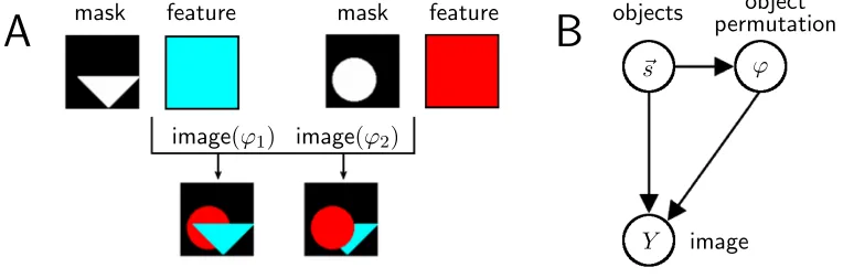
Figure 1: AIllustration of how object masks and features combine to generate an image. If two objects are randomly chosen (|~s|= 2), two different images with two different depth-orders (denoted by ϕ1 and ϕ2) can be generated. B Graphical model of the generation process with hidden variables ~s (object presence) and ϕ (depth permutation).
To model the presence or absence of objects we useHbinary hidden variabless1, . . . , sH. We assume that the presence of one object is independent of the presence of the others and, for simplicity, we also assume that each object is equally likely to be present in an image a priori(we refer to this probability by π). The probability for the presence and absence of objects is given by
p(~s|π) = H Y
h=1
Bernoulli(sh;π) = H Y
h=1
πsh(1−π)1−sh. (1)
Objects in a real image can be ordered by their depth and it is this ordering which determines how the objects occlude each other in regions of overlap. The depth-ordering is captured in the model by associating the active objects with a permutation. We randomly and uniformly choose a member ϕ of the set G(|~s|) which contains all permutation functions ϕ:{˜h1, . . . ,˜h|~s|} → {1, . . . ,|~s|},with |~s|=Phsh, where ˜h1 to ˜h|~s| are the indices of the non-zero entries of~s. More formally, the probability ofϕgiven~s(see Figure 1B) is defined by
A
B
C
sh
h
τ(S, h)
τ
sh
h
τ(S, h)
τ
sh
h
τ(S, h)
τ
Figure 2: Visualization of the mappingτ(S) :{1, . . . , H} →[0,2] which represents different permutations of objects in depth. The eye at the bottom illustrates the position of the observer. A and B show the two possible mappings if two causes are present. Cshows one of the 24 mappings if four causes are present.
Note that we could have defined the prior over the order in depth (Equation 2) independently of~s, by choosing fromG(H) withp(ϕ) = H1!. But then, because the depth of absent objects (sh = 0) is irrelevant, no more than|~s|! distinct choices ofϕwould have resulted in different images.
The final stage of the generative model describes how to produce the image given a selection of active causes and an ordering in relative depth of these causes. One approach would be to choose the closest object and to set the image equal to the feature vector associated with this object. However, this would mean that every image generated from the model would comprise just one object: the closest. What is missing from this description is a notion of the extent of an object and the fact that it might only contribute to a subset of pixels in an image. For this reason, our model contains two sets of object parameters. One set of parameters,W ∈RH×D, describes whether an object contributes to a pixel and the strength of that contribution (D is the number of pixels). The vector (Wh1, . . . , WhD) is therefore described as the maskof object h. If an object is highly localized, this vector will contain many zero elements. The other set of parameters, T ∈RH×C, represents the features of the objects. We define one vectorial feature per objecth,T~h∈RC, describing, for instance, the object’s RGB color (C = 3 in that case). Figure 1A illustrates the combination of masks and features, and Figure 1B shows the graphical model of the generation process. Let us formalize how an image is generated given the parameters W and T and given the hidden variables S = (~s, ϕ). To further abbreviate the notation, we will denote all the model’s parameters by Θ = (W, T, π, σ). We define the generation of a noiseless image
~
T(S,Θ) to be given by the following equations:
~
Td(S,Θ) = WhodT~ho
where ho = argmaxh{τ(S, h)Whd},
τ(S, h) =
0 ifsh = 0 3
2 ifsh = 1 and |~s|= 1 ϕ(h)−1
|~s|−1 + 1 otherwise
In Equation 3 the order in depth is represented by the mapping τ which intuitively can be thought of as the relative proximity of the objects. The form of this mapping has been chosen to facilitate later algebraic steps. To illustrate the combination rule of Equation 3 and the mapping τ consider Figure 1A and Figure 2. Let us assume that the mask values Whd are zero or one (although we will later also allow for continuous values). As depicted in Figure 1A an object h with sh = 1 occupies all image pixels with Whd = 1 and does not occupy pixels with Whd= 0. For all pixels with Whd = 1 the vectorT~h sets the pixels’ values to a specific feature, e.g., to a specific color. The functionτ maps all causesh with sh = 0 to zero while all other causes are mapped to values within the interval [1,2] (see Figure 2). In this way, it assigns a proximity value τ(S, h)>0 to each present object. For a given pixel d the combination rule in Equation 3 simply states that of all objects with Whd = 1, the most proximal is used to set the pixel property. The interval [1,2] represents a natural choice for proximity values, but any interval with boundaries greater zero would result in an equivalent generative process.
Given the latent variables and the noiseless image T~(S,Θ), we take the observed vari-ablesY = (~y1, . . . , ~yD) to be drawn independently from a Gaussian distribution, i.e.,
p(Y|S,Θ) = D Y
d=1
p(~yd|T~d(S,Θ)), p(~y|~t) = N(~y;~t, σ21). (4)
Equations 1 to 4 represent a model for image generation that incorporates occlusion. We will refer to the model as the Occlusive Components Analysis (OCA) generative model.
3. Maximum Likelihood
One approach to learning the parameters Θ = (W, T, π, σ) of this model from data
Y ={Y(n)}n=1,...,N is to use maximum likelihood learning, that is,
Θ∗ = argmaxΘ{L(Θ)} with L(Θ) = log p(Y(1), . . . , Y(N)|Θ)
. (5)
However, as there is usually a large number of objects that can potentially be present in the training images, and since the likelihood involves summing over all combinations of objects and associated orderings, the computation of Equation 5 is typically intractable. More concretely, givenH components the number of different sets of objects that may be present scales with 2H. Occlusion adds additional complexity: for any subset of sizeγ0 of theH objects that may be present there areγ0! different depth orders. Formally, the total number of hidden states to be considered is given by
Statesexact(H) = H X
γ0=0
H γ0
γ0!. (6)
of these intractabilities within the standard Expectation Maximization (EM) formalism for maximum likelihood learning. First, we will describe how the analytical intractability may be avoided using an approximation that softens the occlusion non-linearity, and which therefore allows parameter update equations (M-step equations) to be derived. Second, we will describe how the computational intractability can be addressed by leveraging the sparsity of visual scenes to reduce the space of solutions entertained by the posterior.
To find the maximum-likelihood parameters Θ∗, at least approximately, we use the EM formalism in the form used by Neal and Hinton (1998) and introduce the free-energy functionF(Θ, q) which is a function of Θ and of an unknown distribution q(S(1), . . . , S(N)) over the hidden variables. F(Θ, q) is a lower bound of the likelihoodL(Θ). Approximations introduced later on can be interpreted as constraining the functionq to lie within a specified class. In the model described above each image is assumed to be drawn independently and identically from an underlying distribution, q(S(1), . . . , S(N)) =Q
nqn(S(n),Θ0), which results in the free-energy
F(Θ, q) = N X
n=1
X
S
qn(S; Θ0) h
log p(Y(n)|S,Θ)
+ log p(S|Θ)i
+H[q], (7)
where the function H[q] =−P n
P
Sqn(S; Θ0) log(qn(S; Θ0)) (the Shannon entropy) is in-dependent of Θ. Note that P
S in Equation 7 sums over all possible states of S = (~s, ϕ), i.e., over all binary vectors and all associated permutations in depth, so that the num-ber of terms in the sum is given by Equation 6. These large sums are the source of the computational intractability. In the EM scheme, F(Θ, q) is maximized alternately with respect to the distribution q in the E-step (while the parameters Θ are kept fixed) and with respect to parameters Θ in the M-step (while q is kept fixed). Θ0 refers to the model parameters of the previous iteration of the algorithm. At the end of the M-step, we thus set Θ0 ← Θ. Each EM iteration increases the free-energy or leaves it unchanged. If q is unconstrained (or if any constraints imposed allow it) then the optimal setting of q in the E-step is given by the posterior distribution over the hidden states at the current parameter settings qn(S; Θ0) = p(S|Y(n),Θ0). In this case, each EM step increases the likelihood or leaves it unchanged and this process converges to a (local) maximum of the likelihood.
3.1 M-Step Equations
The M-step of EM, in which the free-energy,F, is optimized with respect to the parameters, is usually derived by taking derivatives ofF with respect to the parameters. Unfortunately, this standard procedure is not directly applicable because the occlusive combination rule in Equation 3 is not differentiable. However, it is possible to soften the combination rule using the differentiable approximation
~
Tρd(S,Θ) := PH
h=1(τ(S, h)Whd)ρWhdT~h PH
h=1(τ(S, h)Whd)ρ
, (8)
states combine in the sense of a softmax operation, and different interval boundaries for the proximity valuesτ(S, h) change how strongly the closest cause dominates the others. Such effects can be counteracted by choosing corresponding finite values forρ, however. For large values ofρ, differences due to different intervals become negligible again.
~
Tρ
d(S,Θ) is differentiable w.r.t. the parametersWhd andThc (withc∈ {1, . . . , C}). For largeρ, the derivatives can be well approximated as follows:
∂ ∂Wid
~
Tρ
d(S,Θ) ≈ Aρid(S, W)T~i,
∂ ∂Tc
i
~
Tρ
d(S,Θ) ≈ Aρid(S, W)Wid~ec, with
Aρid(S, W) := (τ(S,i)Wid)ρ PH
h=1(τ(S,h)Whd)ρ
,
Aid(S, W) := lim ρ→∞A
ρ
id(S, W),
(9)
where ~ec is a unit vector in feature space with entry equal one at position c and zero elsewhere. The approximations on the left-hand-side above become equalities for ρ → ∞. Given the approximate combination rule in Equation 9, we can compute approximations to the derivatives ofF(Θ, q). For large values of ρ the following holds (see Appendix B):
∂ ∂Wid
F(Θ, q)≈
N X n=1 X S
qn(S; Θ0)
∂ ∂Wid
~
Tρd(S,Θ) T
~ f
~
y(n), ~Tρd(S,Θ)
, (10)
∂
∂TicF(Θ, q)≈
N X n=1 X S
qn(S; Θ0) D X
d=1
∂ ∂Tic
~
Tρd(S,Θ) T
~ f
~
y(n), ~Tρd(S,Θ)
, (11)
where f~(~y(n), ~t) := ∂ ∂~t log
p(~y(n)|~t) = −σ−2(~y(n)−~t).
Setting the derivatives in Equations 10 and 11 to zero and inserting Equations 9 yields the following necessary conditions for a maximum of the free-energy that hold in the limit ρ→ ∞:
Wid = X
n
hAid(S, W)iqn T~iT ~y (n) d
X
n
hAid(S, W)iq
n T~
T i T~i
, T~i = X
n X
d
hAid(S, W)iqn Wid ~y
(n) d
X
n X
d
hAid(S, W)iq
n (Wid)
2 . (12)
Note that Equations 12 are not straightforward update rules. However, we can use them in the fixed-point sense and approximate the parameters which appear on the right-hand-side of the equations using the values from the previous iteration. For the update note that due to the multiplication of the weights and the mask,WhdT~hin Equation 3, there is degeneracy for the object parameters: givenh, the combinationT~dremains unchanged for the operation
~
Th→T~h/%andWhd→% Whd with%6= 0. This transformation does not leave the selection of the closest object unchanged (selection of ho in Equation 3) because the values of Whd are not binary. To remove the degeneracy and to keep the values of Whd close to zero or one, we rescale after each EM iteration as follows:
Whdnew=Whd/ Wh, T~hnew=WhT~h, where Wh =
1
|I|
X
d∈I
The use ofWhinstead of, e.g.,Whmax= maxd{Whd}is advantageous for some data, although for many other types of dataWhmaxworks equally well. Through the influence of the scaling on the selection of closest objects, small values of Whd tend to be suppressed for larger values of α and converge to zero. In general, we find the algorithm to avoid local optima more frequently if we initialize α at a small value and then slowly increase it over the EM iterations to a value near 12. The index set I thus contains all entriesWhd at first, and only later considers exclusively entries with higher values for normalization. In this way, smaller values are suppressed only when the algorithm is already closer to an optimum than it is in the beginning of learning.
If the derivatives of the free-energy in Equation 7 w.r.t. to σ (data noise) and π (ap-pearance frequency) are set to zero, we obtain through straightforward derivations (see Appendix B) the following two remaining update rules:
σnew = v u u t
1 N DC
N X
n=1 * D
X
d=1 C X
c=1
y(dcn)− Tdc(S,Θ)2 +
qn
, (13)
πnew= 1 HN
N X
n=1
h|~s|iq
n . (14)
3.2 E-Step Equations
The crucial quantities that have to be computed for update Equations 12 to 14 are expec-tation values w.r.t. the variational distributions qn(S; Θ0) in the form
hg(S,Θ)iq
n =
X
S
qn(S; Θ0)g(S,Θ), (15)
whereg(S,Θ) are functions that depend on the latent state and potentially the model pa-rameters. The optimal choice forqn(S; Θ0) is the exact posterior,qn(S; Θ0) =p(S|Y(n),Θ0), which is given by Bayes’ rule,p(S|Y(n),Θ0) = p(Y(n)|S,Θ0)p(S|Θ0)
P
S0p(Y(n)|S0,Θ0)p(S0|Θ0)
, with prior and noise distributions given by the OCA generative model in Equations 1 to 4. Unfortunately, the computation of the expectations or sufficient statistics in Equation 15 becomes compu-tationally intractable in this case because of the large number of states that have to be considered (see Equation 6). To derive tractable approximations, we can, however, make use of typical properties of visual scenes: in any given scene the number of objects which are present is far smaller than the set of all objects that can potentially be present in the scene. As such, the sum over all states in Equation 15 is typically dominated by only a few terms. More specifically, components which are compatible with the observed image are the only ones to make a significant contribution to this sum, whilst components which are incompatible make only a negligible contribution. Consequently, a good approximation to the expectation values in Equation 15 can be obtained by identifying the states which carry high posterior mass and retaining only these states.
space of functions, then the resulting variational EM algorithm is no longer guaranteed to converge to a local maximum of the likelihood. However, it still increases a lower bound on the likelihood, and frequently finds a good approximation to the maximum likelihood solution. The most commonly used constraint is to decompose q into a product of disjoint factors, for instance, one for each possible source object. By contrast, the approach adopted here uses a distribution truncated to a limited setKn of all possible source configurations, i.e,
qn(S; Θ) =
p(S|Y(n),Θ) X
S0∈K n
p(S0|Y(n),Θ)δ(S
∈ Kn) with δ(S∈ Kn) :=
1 ifS ∈ Kn
0 ifS 6∈ Kn , (16)
whereKn is a subset of the space of all states. IfKn, indeed, contains most of the posterior mass given a data point Y(n), then qn(S; Θ) approximates the exact posterior well. The variational approximation qn(S; Θ) is a truncated posterior distribution that allows for the efficient estimation of the necessary expected values. The approximation is, therefore, referred to as Expectation Truncation(ET; L¨ucke and Eggert, 2010) or truncated EM.
In the case of the OCA generative model, we might expect good approximations if we identified a small set of candidate objects which are likely to be present in the scene, and then letKn contain all of the combinations of the candidate objects. By usingqn(S; Θ) in Equation 16 as a variational distribution, the expectation values required for the M-step are of the form
hg(S,Θ)iq
n =
X
S∈Kn
p(S|Y(n),Θ) X
S0∈K n
p(S0|Y(n),Θ)g(S,Θ) = X
S∈Kn
p(S, Y(n)|Θ0)g(S,Θ) X
S0∈K n
p(S0, Y(n)|Θ0). (17)
We compute Kn for a given data point Y(n) in two stages. In the first we use a computa-tionally inexpensive selection orscoring function (see L¨ucke and Eggert, 2010) to identify candidate objects. The selection function Sh Y(n)
seeks to assign high values to states corresponding to objectsh present in the sceneY(n) and low values to states corresponding to objects which are not present. An ideal selection function would be monotonically related to the posterior probability of the object given the current image, but at the same time it would also be efficient to compute. The topH0 states are selected as candidates and placed into an index set In. In the second stage we form the set Kn from the candidate objects. The index set In is used to define the set Kn as containing the states of all likely object combinations, i.e.,
Kn={S| Phsh ≤γ and ∀h6∈In:sh = 0
or P
jsj ≤1}. (18)
As an additional constraint, Kn does not contain combinations of more than γ objects. Furthermore, we make sure that Kn contains all singleton states, which proved beneficial in numerical experiments.
The selection function itself is defined as the squared distance between the observed image and the image generated by thehth component alone,
Sh Y(n)
=−
D X
d=1 C X
c=1
Ycd(n)− Tcd(S(h); Θ) 2
whereS(h):= (~s(h), ϕ) with~s(h) being the state with only the hth object present. Intuitively, the selection function can be thought of as a measure of the log-probability that each singleton state accounts for the current data point (also see Appendix D). Since we are only interested in the relative values of the selection function between the different components, Equation 19 contains only the exponent of the strictly monotonic exponential function without the normalization pre-factors.
3.3 Efficient EM Learning
The M-step Equations 12 to 14 together with the approximation of the expectation values in Equation 17 represent a learning algorithm for the OCA generative model. Its efficiency crucially depends on the approximation parametersH0 andγ as they determine the number of latent states inKnthat have to be considered, that is,
StatesET(H, H0, γ) = γ X
γ0=0
H0
γ0
γ0! + (H−H0). (20)
Because of the preselection of H0 candidates, the combinatorics no longer scales with H. Only the number of singleton states scales linearly withH. Furthermore, the computation of the selection functions scales withH, but for the selection function specified in Equation 19 this scaling is only linear.
by:
Wid= X
n∈M
hAid(S, W)iqnT~iT~yd(n) X
n∈M
hAid(S, W)iqnT~iTT~i
~ Ti =
X
n∈M X
d
hAid(S, W)iqnWid~yd(n) X
n∈M X
d
hAid(S, W)iqn(Wid)2
(21)
σnew= v u u t 1 |M|CD X n∈M * D X d=1 C X c=1
ydc(n)− Tdc(S,Θ)2 +
qn
(22)
πnew= A(π)π B(π)
1
|M|
X
n∈M
h|~s|iq
n with (23)
A(π) = γ X γ0=0 H γ0
πγ0(1−π)H−γ0 and B(π) = γ X γ0=0 γ0 H γ0
πγ0(1−π)H−γ0.
These modified M-step equations can be derived from a truncated free-energy (L¨ucke and Eggert, 2010) of the form
F(q,Θ) = X n∈M
X
S
qn(S; Θ0) log
p(Y(n)|S,Θ)P p(S|Θ) S0∈Kp(S0|Θ)
, (24)
withqn(S; Θ0) given in Equation 16 and with K being the set of all states S with at most
γ non-zero components, K = {S| |~s| ≤ γ}. Details of the derivations of the update rules are given in Appendix B.
As can be observed, the update equations forW,T and σremain essentially unchanged except for averages now running over the subsetMinstead of all data points (Equations 21 and 22). The reason is that the derivatives of the truncated free-energy w.r.t. these param-eters are equal to the derivatives of the original free-energy except for reduced sums. For the derivative w.r.t. the prior parameter, the situation is different. The additional term in the denominator of the logarithm in Equation 24 results in a correction term for the update equation forπ (Equation 23). Intuitively, it is clear that discounting data points with more thanγ components has a direct impact on estimating the mean probability for a component to appear in a data point. The additional term in Equation 23 corrects for this.
To complete the procedure, we must determine the set Mof all data points which are estimated to haveγ active components or fewer. First note that the size of this set can be estimated given the current estimate forπ. It contains an expected number of
Ncut=N X
S,|~s|≤γ
p(S|π) =N
γ X
γ0=0
H γ0
πγ0(1−π)H−γ0
data points (analogously to theπ correction factor in Appendix B.2). Following L¨ucke and Eggert (2010), we now compute for all N data points the sums P
S∈Knp(S, Y
Iterating the M-step (Equations 21 to 23) and the E-step (Equations 17) results in a learning algorithm for the OCA generative model. As will be shown numerically in the next section, the algorithm allows for a very accurate estimation of model parameters based on a strongly reduced number of latent states.
4. Experiments
In order to evaluate the OCA learning algorithm, it has been applied to artificial and real-world data. Artificial data allows for an evaluation based on ground-truth information and for a comparison with other approaches. The use of real-world data enables us to test the robustness of the method.
4.1 Initialization and Annealing
For all data points, a vector~yd∈[0,1]3represented the RGB values of a pixel. In all trials of the experiments we initialized the parametersWhd andThc by independently and uniformly drawing from the interval [0,1]. The parameters for sparseness and standard deviation were initialized as πinit= H1 and σinit= 5, respectively.
Parameter optimization in multiple-cause models is usually a non-convex problem. For the OCA model, the strongly non-linear combination rule seems to result in even more pro-nounced local optima in parameter space than is the case for other models such as sparse coding. To efficiently avoid convergence to local optima, we (A) applied deterministic annealing (Ueda and Nakano, 1998; Sahani, 1999) and (B) added noise to model parame-ters after each EM iteration. Annealing was implemented by introducing the temperature T = β1. The inverse temperature β started near 0 and was gradually increased to 1 as iter-ations progressed. It modified the EM updates by substitutingπ →πβ, (1−π)→(1−π)β, and σ12 →
β
σ2 in all E-step equations. We also annealed the occlusion non-linearity by
set-tingρ= 1−1β; however, onceβ became greater than 0.95 we setρ= 21 and did not increase it further. We ran 100 iterations for each trial of learning. The inverse-temperature was set to β = D2 for the first 15 iterations, then linearly increased to β = 1 over the next 15 iterations, and then kept constant until termination of the algorithm.
Additive parameter noise was drawn randomly from a normal distribution with zero mean. Its standard deviation was initially set to 0.3 for the mask parameters and at 0.05 for the prior and noise parameters. The value was kept constant for the first 10 iterations and then linearly decreased to zero over the next 30 iterations. The degeneracy parameter α was initialized at 0.2 and increased to 0.6 from iteration 25 to 35. The amount of data points used for training was linearly reduced from N toNcut between iteration 15 to 30. Approximation parameters were set toγ = 3 and H0 = 5 unless stated otherwise.
4.2 Evaluation of Optimization Results
40
0
frequency
0.2 0.22 learnedσ 0.28 0.3
A B
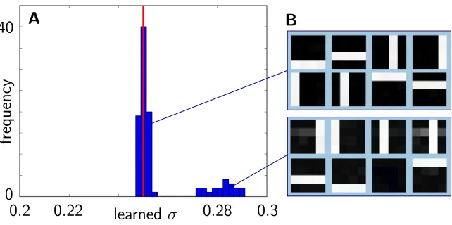
Figure 3: A Histogram of values for the parameter σ (Equation 13) for 100 runs of the algorithm on a standard bars test (see bars test section). The ground-truth value for σ in these runs was 0.25, indicated by the red line. As can be observed, most values lie close to this number while some values form a second mode at higher values. By thresholding the σ parameter, we can identify local optima. BExamples for the basis functions for the left and for the right cluster.
are not known and so another measure for the quality of a run has to be found. A good indication of the quality of the learned parameters is provided by the learned noise parameter σ (Equation 13). In fact, if we compute the derivative of the update rule for σ w.r.t. the mask and feature parameters and set these equal to zero, we obtain the same update rules for W and T as for the derivative of the energy. That is, maximizing the free-energy corresponds to optimizing (minimizing) the noise which the model has to assume to explain the data (see Appendix C). If this noise is small, the data are well explained by the parameters (see Figure 3 for an application to artificial data).
4.3 Colored Bars Test
annealing temperature sparsenessπH
stdσ
parameter noise
0 20 iteration 80 100 0.0
0.3 0.0 0.4 0.8
A C
D
E
F 4.0
1.0 0.0 2.0 4.0
B
Mask
100 50 20 10 5 1 0
Feature Combined Mask and Feature
iteration
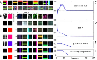
Figure 4: A Example of ten noiseless and noisified data points. B Development of the (reshaped) generative fields for the given iterations. For the first cause, maskW~h and featureT~hT are displayed separately. The other causes are shown as product
~
Wh·T~hT. C-D Development of data sparseness and standard deviation over the 100 iterations. E Magnitude of the noise which is added to the mask parameters after each iteration. FAnnealing temperature as chosen for the algorithm.
reliabilities. In addition to increasing efficiency, Expectation Truncation, therefore, helps in avoiding local optima for this model, presumably because local optima corresponding to broad posterior distributions are avoided. A similar observation was recently reported in an application of ET to a sparse coding variant (Exarchakis et al., 2012).
4.4 Standard Bars Test
Instead of choosing the bar colors randomly as above, they can also be set to specific values. In particular, if all bar colors are white, T~ = (1,1,1)T, the classical version of the bars test is recovered. Note that the learning algorithm can be applied to this standard form without modification, even though it is impossible to recover the relative depth of the bars in this case. When the generating parameters were as above (eight bars, probability of a bar to be present 28,N = 1000), all bars were successfully extracted in 80 of 100 trials (80% reliability). The estimated values of σ and π lay in the intervals [0.247,0.254] and [0.241,0.263], respectively. When learning on noiseless data, we obtained a reliability of 95%. By increasing the approximation parameters toγ = 4 andH0 = 6, reliability changed to 91%.
For a standard setting of the parameters (N = 500,H= 10,D= 5×5, probability of 102 for each bar to be present) as was used in numerous previous studies (Saund, 1995; Dayan and Zemel, 1995; Hochreiter and Schmidhuber, 1999; L¨ucke and Sahani, 2008; L¨ucke and Eggert, 2010), the OCA algorithm with γ = 3 and H0 = 5 achieved 83% for a noisy and 78% for a noiseless bars test. For N = 1000 data points reliability increased to 85%. For comparison, earlier generative modeling approaches such as those reported by Saund (1995) or Dayan and Zemel (1995) (both assuming a noisy-or like combination rule) achieved 27% and 69% reliability, respectively. Maximal Causes Analysis (L¨ucke and Sahani, 2008; L¨ucke and Eggert, 2010) achieved about 82% (MCA3) reliability. And the preliminary version of the OCA algorithm (L¨ucke et al., 2009) achieved 86% for noiseless data. Approaches such as PCA or ICA were reported to fail in this task (Hochreiter and Schmidhuber, 1999). Furthermore, different types of objective functions and neural network approaches (Charles et al., 2002; L¨ucke and Malsburg, 2004; Spratling, 2006) are also successful at this task, often reporting close to 100% reliability (also see Frolov et al., 2014). The assumptions used (e.g., fixed bar appearance, noise level, parameter constraints, constraint on latent activities) are often implicit but, at the same time, can significantly facilitate learning. NMF algorithms can be successful in extracting all bars (with up to 100% reliability) but require hand-set values for sparsity constraints on hidden variables and/or parameters (see Hoyer, 2004, and for discussions Spratling, 2006, L¨ucke and Sahani, 2008). In general, the fewer assumptions a model makes, the more difficult it becomes to infer the parameters from a given set of data. For earlier generative models and in particular for the more general model discussed in this paper, larger data sets directly translate into higher reliabilities. A reliability of 78% for the noiseless bars test is, for the OCA algorithm discussed in this work, in this view still relatively high. Reliabilities are comparable to values for MCA and to the preliminary OCA algorithm (L¨ucke et al., 2009). Note, however, that the latter did use fixed values for data noiseσ and bar appearance π which may explain the higher reliability.
all bars by considering several runs of the algorithm simultaneously. That is, given a set of N images, we can apply the algorithmM times, and use as the final result the parameters of a run with the smallestσvalue. For some data sets, we even obtain two clusters ofσ values (see Figure 3) where the cluster with smallerσ’s represents the runs which have terminated in an optimum with parameters representing all bars. Note that clearly separable clusters are not observed for all data sets and parameter settings. In general, however, runs with small σ values tend to correspond to parameters reflecting the true underlying generative process more accurately. For the standard settings of the bars test withD= 5×5,N = 500, H = 10, and noiseless data, the algorithm with M = 20 extracts all components in 50 of 50 runs. But note that each run now consists of evaluating M = 20 subruns. The same applies for values ofM down toM = 10.
4.5 Inference
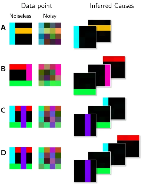
To briefly illustrate the algorithm’s performance on an inference task, i.e., the extraction of the underlying causes and their depth order, and to show how inference can be applied to data points exceeding γ components, let us consider data points generated according to the colored bars test. Furthermore, consider the model after it has learned the parameters to represent the bars, noise level, and sparsity. Given a data point, the trained model can infer the hidden variables by applying the following procedure: We start by executing an E-step with the same values for H0 and γ as used during training (H0 = 5 and γ = 3 in this case). We then determine the maximum a-posteriori (MAP) state ~s∗ based on the approximate posterior computed in this E-step. If this state has|~s∗|=γ active components, we repeat the E-step with values of H0 andγ increased by one each (leavingH0 unchanged if H0 = H). We terminate the procedure if the MAP state has less than γ states or if γ = H0 = H. Exemplarily, Figure 5 shows three data points and the corresponding MAP states obtained with the described procedure. The data point with two components terminated after the first E-step (Figure 5A), the data points with three afterγwas increased to four (Figure 5B), and the data point with four components terminated after γ was increased to five (Figure 5C,D show result for initial and final γ). For ambiguous data points, e.g., if the input contained two parallel bars, two states or more states can carry equally large probability mass due to the fact that different depth permutations do not change the image. The MAP estimate can still serve to illustrate the inference result but the approximate distribution over states represents a more accurate description in this case.
4.6 More Realistic Data
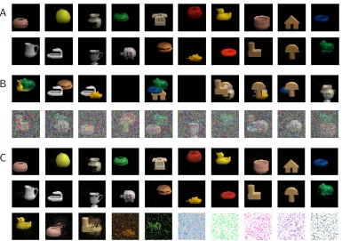
To numerically investigate the algorithm for more realistic data, it was applied to data based on pictures of objects from the COIL-100 database (Nene et al., 1996).1 Images were scaled down to 20×20 pixels and were placed at random planar positions on a black background image ofD= 35×35 = 1225 pixels. The objects were then colored with their mean color, weighted by pixel intensity (see Figure 6A). In 100 runs, we created N = 8000 data points by combiningHgen= 20 of these images according to the generative model with
Noiseless Noisy
Data point Inferred Causes
C B A
D
Figure 5: Examples of the inference procedure for the colored bars test. The second column shows the data points used for inference (with their noiseless versions in the first column). On the right, the causes inferred from the noisy data points are shown arranged in their inferred depth order. A - D The algorithm reliably inferred the causes for the three examples (C and D show two steps of the inference procedure). Note that we have learned the basis functions from noisy data with the same properties as those shown here.
prior parameter π = H2
gen = 0.1, i.e., πHgen = 2 and data noise σ = 0.25 (see Figure 6B).
B A
C
Figure 6: A20 downscaled COIL images. B10 noiseless and 10 noisy data points (obtained fromA according to Equation 3). C30 extracted basis functions. The first two rows display the clean extracted causes in the same order as in A. The third row shows the additionally learned causes which are mostly noisy fields or noisy combinations of more than one cause.
represented. Again, low values of the observation noise were found to indicate the successful extraction of all objects. By performing a series of runs and retaining the parameters of runs with the lowest learned observation noise, the reliability increased to close to 100%.
4.7 Real Data
A
1
5
10
15
30 0 D Iteration
C B
x y
Figure 7: Numerical experiment with photographic images of cars. A Five cars could ap-pear in three lanes which account for the arbitrary position in depth (y). Position in x-direction was fixed. BOne of the 500 pictures taken of one state with three active causes. C 10 data points after cutting and pre-processing. D Generative fields (mask on top, feature below) at different iterations.
iterations 15 and 26. Over 30 iterations we extracted the masks of all five cars along with data noise (σ= 0.05) and sparseness (π = 0.17 withπground-truth = H1 = 0.2). The features which had positive and negative values were mapped to [0,1] to be interpreted as color. As can be seen from the generative fields in iteration 30, not all masks were extracted cleanly. This can be explained by the fact that a different position in depth still causes a slight shift in planar space such that in some images one cause is higher or lower than in others. This smearing effect leads to a change in color because a pixel then sometimes belongs to the car and sometimes to the background which results in a color shift towards the background color (black). Another reason is that one cause does not only consist of one color but rather of a combination of the car color and background, shadow, window, and wheel color. For the yellow car which is relatively similar to the background the mask almost only represents the shadow of the car, which is the most salient part relative to the background. For the other cars, the masks correspond to representations of whole cars.
5. Discussion
We have studied learning in a multiple-cause generative model which assumes an explicit model of occlusion for component superposition. According to the OCA model assumptions, an object can appear in different depth positions for different images. This aspect reflects properties of real images and is complementary, e.g., to assumptions made by sprite models (Jojic and Frey, 2001; Williams and Titsias, 2004). A combination of sprite models and the OCA model is, therefore, a promising line of inquiry, e.g., towards systems that can learn from video data in which objects change their positions in depth. Other lines of research have also identified occlusions as an important property that has to be modeled for applications to visual data. In the context of neural network modeling, Tajima and Watanabe (2011) have recently addressed the problem (albeit with a very small number of components and in a partly supervised setting), while restricted Boltzmann machines have been augmented by LeRoux et al. (2011) to incorporate occlusions.
our model, the combination of masks and vectorial feature parameters, furthermore, allows for applications to more general sets of data than the scalar values used for SC, NMF or than in applications of sprite models (compare Jojic and Frey, 2001; Williams and Titsias, 2004). In numerical experiments we have used color images for instance. However, we can also apply our algorithm to gray-level data such as used for other algorithms. This allows for a direct quantitative comparison of the novel algorithm with state-of-the-art component extraction approaches. The reported results for the standard bars test show the competitiveness of our approach despite its larger set of parameters (compare, e.g., Spratling, 2006; L¨ucke and Sahani, 2008). For applications to visual data, color is the most straightforward feature to model. Possible alternatives are Gabor feature vectors which model object edges and textures, or further developments such as SIFT features (Lowe, 2004). Depending on the application, the generative model itself could also be generalized. It is, for instance, straightforward to introduce several feature vectors per cause. Although one feature (e.g., one color) per cause can represent a suitable model for many applications, it might for other applications also make sense to use multiple feature vectors per cause. In the extreme case, as many feature vectors as pixels could be used, i.e., T~h → T~hd. The derivation of update rules for such features would proceed along the same lines as the derivations for single features T~h. Furthermore, individual prior parameters for the frequency of object appearances could be introduced. Additional parameters could be used to model different prior probabilities for different arrangements in depth. Finally, the most interesting but also most challenging generalization direction would be the inclusion of explicit invariance models. In its current form the model uses, in common with state-of-the-art component extraction algorithms, the assumption that the component locations are fixed. Especially for images of objects, changes in planar component positions have to be addressed in general. Possible approaches that have been discussed in the literature have, for instance, been investigated by Jojic and Frey (2001) and Williams and Titsias (2004) in the context of occlusion modeling, by Eggert et al. (2004) and Wersing and K¨orner (2003) in the context of NMF, or by Berkes et al. (2009), Gregor and LeCun (2011) and others in the context of sparse coding. The crucial challenge of a generalization of the occlusion model studied in this work is the further increase in the dimensionality of the hidden space. By generalizing the methods as used here, such challenges could be overcome, however. On the other hand, methods such as sparse coding or NMF have proven to be useful building blocks in vision systems although they do not address translation invariance in an explicit way. As a generalization of sparse coding, the model studied here can provide a more accurate model in situations where the modeling of occlusions is important. Like for sparse coding, no prior information about the two dimensional nature of images is used in the model, i.e., learning would not suffer from a (fixed) permutation of all pixels applied to all data points. The tasks faced by the model may, therefore, appear easier for the human observer because humans make (e.g., for the COIL data) use of additional object knowledge such as of the gestalt law of proximity. This also illustrates that extensions of the model to incorporate prior knowledge about objects would further improve the approach.
be overcome. Replacing the standard linear superposition of sparse coding by an occlusion superposition resulted in a number of challenges that all had to be addressed:
1) The occlusion model required parameterized masks.
2) The learning equations are not closed-form.
3) Occlusion leads to a much larger combinatorial explosion of possible configurations.
4) Posterior probabilities are not unimodal.
5) Local optima in parameter space are more pronounced.
had an influence on the typical convergence points. With only parameter noise (i.e., with-out annealing), the algorithm usually converged within few EM iterations to local optima with a relatively large number of fields representing more than one component. With only annealing (i.e., without parameter noise), the algorithm often converged to local optima in which most components were represented correctly but where few generative fields repre-sented two components. The combination of annealing and parameter noise resulted in a frequent representation of all causes (see experiments). As stated earlier, we also observed a positive effect of the approximation scheme in avoiding local optima presumably because shallow local optima corresponding to solutions with dense states are not considered by the truncated approximation.
A further improvement that followed from the application of Expectation Truncation is the availability of learning rules for data noise and sparsity. While data noise could have been inferred within the preliminary study of the occlusion model (L¨ucke et al., 2009), inference of sparsity requires a correction term that compensates for considering a reduced space of latent configurations, and Expectation Truncation provides a systematic way to derive such a correction (compare Appendix B.2). Data noise and sparsity parameters are, notably, not a consequence of modeling occlusion. They are potential parameters also of standard sparse coding approaches or NMF objective functions. Nonetheless, most sparse coding approaches only optimize the generative fields because of limitations induced by the usual maximum a-posteriori based learning (but see Berkes et al., 2008; Henniges et al., 2010, for exceptions). Likewise, NMF approaches focus on learning of generative fields / basis functions. Sparsity is at most indirectly inferred by standard SC or NMF through cross-validation.
To summarize, our study shows that the challenges of occlusion modeling with explicit depth orders can be overcome, and that all model parameters can be efficiently inferred. The approach complements established approaches of occlusion modeling in the literature by generalizing standard approaches such as sparse coding or NMF to incorporate one of the most salient properties of visual data.
Acknowledgments
Appendix A. Illustration of Hidden State Combinatorics
after preselection
additional singleton:
(example) for data point
StatesET(4,3,2) = 11
StatesET(H, H0, γ) =
γ
X
γ0=0
H0 γ0
γ0! + (H−H0)
γ0= 1
γ0= 2
γ0= 3
γ0= 4
γ0= 0
ET withH = 4,H0= 3, and γ= 2
Exact EM withH = 4
Statesexact(4) = 65
Statesexact(H) =
H
X
γ0=0
H
γ0
γ0!
Appendix B. Derivation of Update Rules
Our goal is to optimize the free-energy, i.e.,
F(Θ, q) = N X n=1 X S
qn(S; Θ0) h
log p(Y(n)|S,Θ)+ log p(S|Θ) i
+ H[q],
where
p(Y(n)|S,Θ) = D Y
d=1
p(~yd(n)|T~d(S,Θ)) withp(~y|~t) =N(~y;~t, σ21).
More explicitly,
p(Y(n)|S,Θ) = D Y d=1 C Y c=1 1 √
2πσ2 exp
− 1
2σ2
y(cdn)− Tcd(S,Θ) 2
= 2πσ2−
CD 2 D Y d=1 C Y c=1 exp − 1
2σ2
ycd(n)− Tcd(S,Θ) 2
and for the logarithm
log
p(Y(n)|S,Θ)
=−CD
2 log 2πσ 2 − D X d=1 C X c=1 1 2σ2
y(cdn)− Tcd(S,Θ) 2
.
The prior term, we defined to be
p(S|Θ) =π|~s|(1−π)(H−|~s|) 1
|~s|!,
such that
log (p(S|Θ)) =|~s|log(π) + (H− |~s|) log(1−π)−
|~s| X
γ=1
log(γ).
The free-energy thus takes the form
F(Θ, q) = N X n=1 X S
qn(S; Θ0)
−CD
2 log 2πσ 2
− 1
2σ2 D X d=1 C X c=1
y(cdn)− Tcd(S,Θ)2
+|~s|log(π) + (H− |~s|) log(1−π)−
|~s| X
γ=1 log(γ)
B.1 Optimization of the Data Noise
Let us start be deriving the M-step equation forσ as follows:
∂
∂σF(Θ, q)
= N X n=1 X S
qn(S; Θ0)
−CD
2 ∂
∂σlog 2πσ 2 − ∂ ∂σ 1 2σ2
D X d=1 C X c=1
ycd(n)− Tcd(S,Θ)
2 = N X n=1 X S
qn(S; Θ0)
−CD
2 4πσ
2πσ2 −(−2 (2σ) −32) D X d=1 C X c=1
ycd(n)− Tcd(S,Θ)2 = N X n=1 X S
qn(S; Θ0)
−CD
σ +
1 2σ3
D X d=1 C X c=1
ycd(n)− Tcd(S,Θ)2
! = 0
⇒ 1
2σ3 N X n=1 X S
qn(S; Θ0) D X d=1 C X c=1
ycd(n)− Tcd(S,Θ)2
= N CD σ
⇒σ2 = 1 N CD N X n=1 X S
qn(S; Θ0) D X d=1 C X c=1
y(cdn)− Tcd(S,Θ)2
For ET, all we need to change is the amount of data points we consider. We thus obtain for the update of the data noise that
σnew = v u u t 1 |M|CD X n∈M * D X d=1 C X c=1
y(dcn)− Tdc(S,Θ)2 +
qn
.
B.2 Optimization of the Prior Parameter
Now we will derive the M-Step equation for the update of the parameter π as follows:
∂
∂πF(Θ, q) =
N X n=1 X S
qn(S; Θ0)
∂
∂π|~s|log(π) + ∂
∂π(H− |~s|) log(1−π) = N X n=1 X S
qn(S; Θ0)
|~s|
π −
H− |~s|
1−π = N X n=1 X S
qn(S; Θ0)
|~s| −Hπ π(1−π)
! = 0 ⇒ N X n=1 X S
qn(S; Θ0)|~s|=HπN
⇒ π= 1
N H N X n=1 X S
With ET, we have to introduce a normalization factor, A, which changesp(S|π) to
pET(S|π) = (1
Ap(S|π), |~s| ≤γ 0, |~s|> γ .
WithP
SpET(S|π) = P
S∈Kn
1
Ap(S|π)≈ P
S;|~s|<γ 1
Ap(S|π) !
= 1, we find that
A= X
S,|~s|≤γ
p(S|π) = X S,|~s|≤γ
π|~s|(1−π)(H−|~s|) 1
|~s|!
=1×π0(1−π)H +H×π1(1−π)(H−1) +H(H−1)×π2(1−π)(H−2)1
2!+. . .
= γ X
γ0=0
H γ0
πγ0(1−π)H−γ0.
As we are going to need it below, we define
B(π) := γ X
γ0=0
γ0
H γ0
πγ0(1−π)H−γ0
and also calculate the derivative of Aw.r.t. π as follows:
∂
∂πA(π) =
γ X
γ0=0
H γ0 γ0 π π γ0
(1−π)(H−γ0)−πγ0(1−π)(H−γ0)H−γ 0
1−π
= γ X
γ0=0
H γ0 π
γ0
(1−π)(H−γ0)
γ0 π −
H 1−π +
γ0 1−π
=1 π
γ X
γ0=0
γ0
H γ0
πγ0(1−π)(H−γ0)
− H
1−π
γ X
γ0=0
H γ0
πγ0(1−π)(H−γ0)
+ 1 1−π
γ X
γ0=0
γ0
H γ0
πγ0(1−π)(H−γ0)
=1
πB(π)− H
1−πA(π) + 1
1−πB(π)
= B(π) π(1−π)−
As we now take the derivative of the ET prior, we find that
∂
∂πlog (pET(S|π)) = ∂ ∂πlog
1 A(π)π
|~s|(1−π)(H−|~s|) 1
|~s|!
= |~s| π −
H− |~s|
1−π − ∂
∂πlogA(π)
= |~s| π −
H− |~s|
1−π − 1 A(π)
∂ ∂πA(π)
= |~s| π −
H− |~s|
1−π −
B(π) A(π)π(1−π) +
H 1−π
= |~s| π −
H 1−π +
|~s|
1−π −
B(π) A(π)π(1−π) +
H 1−π
= |~s| π(1−π) −
B(π) A(π)π(1−π).
We now have to set the free-energy with this expression equal to zero:
X
n∈M X
S∈Kn
q(n)(S,Θ0)
|
~s|
π(1−π) −
B(π) A(π)π(1−π)
! = 0 ⇒ X n∈M X
S∈Kn
q(n)(S,Θ0)|~s|= B(π)|M| A(π)
⇔ A(π)
B(π)|M|
X
n∈M X
S∈Kn
q(n)(S,Θ0)|~s|= 1
In a fixed-point sense, this expression can be multiplied with π on both sides, one repre-senting the updatedπnew and one the oldπ from the iteration before:
πnew=
A(π)π B(π)
1
|M|
X
n∈M
h|~s|iq n
B.3 Optimization of the Basis Functions
For the M-step equations of the mask and feature parameters, we observe that
∂ ∂Wid
F(Θ, q) = 1 2σ2
N X
n=1 X
S
qn(S; Θ0)
∂ ∂Wid D X d=1 C X c=1
y(cdn)− Tcd(S,Θ)2
=− 1
σ2 N X n=1 X S
qn(S; Θ0) C X
c=1
ycd(n)− Tcd(S,Θ)
∂
∂Wid
Tcd(S,Θ)
and
∂ ∂Tic
F(Θ, q) = 1 2σ2
N X
n=1 X
S
qn(S; Θ0)
∂ ∂Tic D X d=1 C X c=1
ycd(n)− Tcd(S,Θ) 2
=− 1
σ2 N X n=1 X S
qn(S; Θ0) D X
d=1
ycd(n)− Tcd(S,Θ)
∂
∂Tic
We thus have to calculate the derivative of the combination rule. Since the original non-linear combination rule is not differentiable, we calculate the derivative of the approximated function and find that
∂ ∂Wid
Tcdρ(S,Θ) = ∂ ∂Wid
PH
h=1(τ(S, h)Whd)ρWhdThc PH
h=1(τ(S, h)Whd)ρ
= u 0v
v2 − uv0
v2
=(τ(S, i)Wid) ρT
ic(ρ+ 1)×PHh=1(τ(S, h)Whd)ρ
PH
h=1(τ(S, h)Whd)ρ 2
−
PH
h=1(τ(S, h)Whd)ρWhdThc×ρ(τ(S, i)Wid)ρ−1τ(S, i)
PH
h=1(τ(S, h)Whd)ρ 2
=(τ(S, i)Wid) ρT
ic(ρ+ 1) PH
h=1(τ(S, h)Whd)ρ
− Tcdρ(S,Θ)×ρ(τ(S, i)Wid)ρ−1τ(S, i)
=. . . .
As this derivation does not result in an analytically tractable solution, we introduce another approximation: The prefactor (τ(S, h)Whd)ρ together with the normalizing denominator PH
h=1(τ(S, h)Whd)ρsimulates a differentiable step-function, i.e., its derivative will be zero almost everywhere, except for close to the point where the actual ’step’ is where it is infinitely large. We will thus treat this entity as a constant prefactor. We obtain that
∂ ∂Wid
Tcdρ(S,Θ) = PH
h=1(τ(S, h)Whd)ρ∂W∂idWhdThc PH
h=1(τ(S, h)Whd)ρ = (τ(S, i)Wid)
ρT ic PH
h=1(τ(S, h)Whd)ρ =Aρid(S, W)Tic,
where we defined for convenience that
Aρid(S, W) := (τ(S, i)Wid) ρ
PH
h=1(τ(S, h)Whd)ρ
withAid(S, W) := lim ρ→∞A
ρ
id(S, W).
For the feature parameter, we find that
∂ ∂Tic
Tcdρ(S,Θ) =Aρid(S, W)Wid.
For largeρ, we find for a well-behaved functionf(t) that
Aρid(S, W)f(Tcdρ(S,Θ))≈ Aρid(S, W)f(WidTic).
When we insert this, together with the derivations above, into the free-energy, we observe that
∂ ∂Wid
F(Θ, q) = 1 σ2
N X
n=1
X
S
qn(S; Θ0) C X
c=1
ycd(n)−WidTic
Aρid(S, W)Tic
and
∂ ∂Tic
F(Θ, q) = 1 σ2 N X n=1 X S
qn(S; Θ0) D X
d=1
y(cdn)−WidTic
Aρid(S, W)Wid
! = 0.
Then it follows that
N X
n=1 X
S
qn(S; Θ0)Aidρ(S, W)T~iT~y (n)
d = N X n=1 X S
qn(S; Θ0)Aρid(S, W)WidT~iTT~i
and N X n=1 X S
qn(S; Θ0) D X
d=1
Aρid(S, W)ycd(n)Wid= N X
n=1 X
S
qn(S; Θ0) D X
d=1
Aρid(S, W)Tic(Wid)2.
After a transformation, we find that
N X
n=1
Aρid(S, W) qn
~
TiT~yd(n)=Wid N X
n=1
Aρid(S, W) qn
~ TiTT~i
and N X n=1 D X d=1
Aρid(S, W) qny
(n)
cd Wid=Tic N X n=1 D X d=1
Aρid(S, W)
qn(Wid)
2.
Solving for the feature and mask parameters, we then obtain the necessary conditions for a maximum of the free-energy that need to hold in the limit ρ → ∞. They are given as follows:
Wid= N X
n=1
Aρid(S, W)q
n
~ TiT~yd(n)
N X
n=1
Aρid(S, W)q
n
~ TiTT~i
and
Tic= N X n=1 D X d=1
Aρid(S, W)q
nWidy
(n) cd N X n=1 D X d=1
Aρid(S, W)
qn(Wid)
2 .
For ET, we need to restrict the sums over the data points to only those summands corre-sponding to data points which can be expected to be explained by less or equalγ causes, i.e., data points which are in the setM. The resulting update equations are given as follows:
Widnew= X
n∈M
hAid(S, W)iqnT~
T i ~y
(n) d
X
n∈M
hAid(S, W)iqnT~
T i T~i
, T~inew= X
n∈M X
d
hAid(S, W)iqnWid~y
(n) d
X
n∈M X
d
hAid(S, W)iqn(Wid)
Appendix C. Influence of the Basis Functions on the Data Noise
Notably, as we alter the mask and feature values during learning, these new values have an effect on the value for σ. More specifically, we have seen that optimization runs resulting in low values for sigma closely correspond to a representation of the true underlying causes while runs with comparably high sigma values do not. For data such as provided by the bars test the final sigma values for different runs may even form corresponding clusters (Figure 3). The interplay between sigma values and object parameters will be investigated here in more detail: As we compare the derivative of the free-energy w.r.t. the masks and features
∂ ∂Wid
F(Θ, q) =− 1
σ2 N X n=1 X S
qn(S; Θ0) D X d=1 C X c=1
y(cdn)− Tcd(S,Θ) ∂ ∂Wid
Tcd(S,Θ)
and
∂ ∂Tic
F(Θ, q) =− 1
σ2 N X n=1 X S
qn(S; Θ0) D X d=1 C X c=1
y(cdn)− Tcd(S,Θ)
∂
∂Tic
Tcd(S,Θ)
with the derivative of the obtained update rule for the data noise squared, again w.r.t. both basis function parameters
∂ ∂Wid
σ2 = 2 N CD N X n=1 X S
qn(S; Θ0) D X d=1 C X c=1
ycd(n)− Tcd(S,Θ)
∂
∂Wid
Tcd(S,Θ)
∂ ∂Tic
σ2 = 2 N CD N X n=1 X S
qn(S; Θ0) D X d=1 C X c=1
ycd(n)− Tcd(S,Θ)
∂
∂Tic
Tcd(S,Θ)
we find that these are virtually identical, except for a pre-factor which will disappear when we set the derivatives equal to zero. The optimal values for the mask and feature vectors in terms of the free-energy thus also optimize the data noise.
Appendix D. Selection Function
A straightforward selection function is given by the posterior for only one active cause which we calculate through Bayes’ rule as, i.e.,
p(Sh|Y(n),Θ) =
p(Y(n)|Sh,Θ)p(Sh|Θ)
p(Y(n)|Θ)
whereS(h):= (~s(h), ϕ) with~s(h) being the state with only the hth object present. Since we are only interested in comparing the numbers per data point, a normalization w.r.t. p(Y(n)|Θ) is not required and does not have to be calculated for the selection function. Since the priorp(Sh|Θ) is identical for allSh, we can omit that entity as well. We are, therefore, left with only the noise (or likelihood) term, i.e.,
p(Y(n)|Sh,Θ) = 2πσ2 −CD 2 D Y d=1 C Y c=1 exp − 1
2σ2
ycd(n)− Tcd(Sh,Θ) 2
Since the logarithm is a strictly monotonic function, we instead can consider
log
p(Y(n)|Sh,Θ)
=−CD
2 log 2πσ 2
− 1
2σ2 D X
d=1 C X
c=1
y(cdn)− Tcd(Sh,Θ) 2
.
As the first term is constant for all causes, as is the prefactor − 1
2σ2, we omit these and are
then left with
Sh Y(n) =−
D X
d=1 C X
c=1
y(cdn)− Tcd(Sh; Θ) 2
,
which is the function used to select the most likely hidden units given Y(n) (compare Equation 19).
References
P. Berkes, R. Turner, and M. Sahani. On sparsity and overcompleteness in image models. In Advances in Neural Information Processing Systems, volume 20, pages 89–96, 2008.
P. Berkes, R. E. Turner, and M. Sahani. A structured model of video reproduces primary visual cortical organisation. PLOS Computational Biology, 5(9):e1000495, 2009.
J. Bornschein, M. Henniges, and J. L¨ucke. Are V1 receptive fields shaped by low-level visual occlusions? A comparative study. PLOS Computational Biology, 9(6):e1003062, 2013.
D. Charles, C. Fyfe, D. MacDonald, and J. Koetsier. Unsupervised neural networks for the identification of minimum overcomplete basis in visual data. Neurocomputing, 47(1-4): 119–143, 2002.
P. Dayan and R. S. Zemel. Competition and multiple cause models. Neural Computation, 7:565 – 579, 1995.
C. Eckes, J. Triesch, and C. von der Malsburg. Analysis of cluttered scenes using an elastic matching approach for stereo images. Neural Computation, 18(6):1441–1471, 2006.
J. Eggert, H. Wersing, and E. K¨orner. Transformation-invariant representation and NMF. In 2004 IEEE International Joint Conference on Neural Networks, pages 2535–39, 2004.
G. Exarchakis, M. Henniges, J. Eggert, and J. L¨ucke. Ternary sparse coding. InProceedings LVA/ICA, pages 204–212, 2012.
P. F¨oldi´ak. Forming sparse representations by local anti-Hebbian learning. Biological Cy-bernetics, 64:165–170, 1990.
A. A. Frolov, D. Husek, and P. Y. Polyakov. Two expectation-maximization algorithms for Boolean factor analysis. Neurocomputing, 130:83–97, 2014.
K. Gregor and Y. LeCun. Efficient learning of sparse invariant representations. CoRR, abs/1105.5307, 2011.
M. Henniges, G. Puertas, J. Bornschein, J. Eggert, and J. L¨ucke. Binary sparse coding. In Proceedings LVA/ICA, LNCS 6365, pages 450–57. Springer, 2010.
S. Hochreiter and J. Schmidhuber. Feature extraction through LOCOCODE. Neural Com-putation, 11:679–714, 1999.
A. Honkela and H. Valpola. Unsupervised variational Bayesian learning of nonlinear models. InAdvances in Neural Information Processing Systems, volume 17, pages 593–600, 2005.
P. O. Hoyer. Non-negative matrix factorization with sparseness constraints. Journal of Machine Learning Research, 5:1457–69, 2004.
N. Jojic and B. Frey. Learning flexible sprites in video layers. In IEEE Conference on Computer Vision and Pattern Recognition, pages 199–206, 2001.
D. D. Lee and H. S. Seung. Learning the parts of objects by non-negative matrix factoriza-tion. Nature, 401(6755):788–91, 1999.
N. LeRoux, N. Heess, J. Shotton, and J. Winn. Learning a generative model of images by factoring appearance and shape. Neural Computation, 23:593–650, 2011.
D. Lowe. Distinctive image features from scale-invariant keypoints. International Journal of Computer Vision, 60(2):91–110, 2004.
J. L¨ucke and J. Eggert. Expectation truncation and the benefits of preselection in training generative models. Journal of Machine Learning Research, 11:2855–900, 2010.
J. L¨ucke and C. Malsburg. Rapid processing and unsupervised learning in a model of the cortical macrocolumn. Neural Computation, 16:501–33, 2004.
J. L¨ucke and M. Sahani. Maximal causes for non-linear component extraction. Journal of Machine Learning Research, 9:1227–67, 2008.
J. L¨ucke, R. Turner, M. Sahani, and M. Henniges. Occlusive components analysis. In Advances in Neural Information Processing Systems, volume 22, pages 1069–77, 2009.
R. Neal and G. Hinton. A view of the EM algorithm that justifies incremental, sparse, and other variants. In M. I. Jordan, editor, Learning in Graphical Models. Kluwer, 1998.
S. Nene, S. Nayar, and H. Murase. Columbia object image library (COIL 100). 1996.
B. Olshausen and D. Field. Emergence of simple-cell receptive field properties by learning a sparse code for natural images. Nature, 381:607–9, 1996.
M. Sahani. Latent Variable Models for Neural Data Analysis. PhD thesis, Caltech, 1999.
E. Saund. A multiple cause mixture model for unsupervised learning. Neural Computation, 7:51–71, 1995.
M. Spratling. Learning image components for object recognition. Journal of Machine Learning Research, 7:793–815, 2006.
S. Tajima and M. Watanabe. Acquisition of nonlinear forward optics in generative models: Two-stage ”downside-up” learning for occluded vision. Neural Networks, 24(2):148–58, 2011.
R. Turner and M. Sahani. Two problems with variational expectation maximisation for time-series models. In D. Barber, T. Cemgil, and S. Chiappa, editors, Bayesian time series models, chapter 5, pages 109–130. Cambridge University Press, 2011.
N. Ueda and R. Nakano. Deterministic annealing EM algorithm. Neural Networks, 11(2): 271–82, 1998.
H. Valpola and J. Karhunen. An unsupervised ensemble learning method for nonlinear dynamic state-space models. Neural Computation, 14(11):2647–2692, 2002.
T. ˇSingliar and M. Hauskrecht. Noisy-or component analysis and its application to link analysis. Journal of Machine Learning Research, 7:2189–2213, 2006.
H. Wersing and E. K¨orner. Learning optimized features for hierarchical models of invariant object recognition. Neural Computation, 15(7):1559–88, 2003.
C. K. I. Williams and M. K. Titsias. Greedy learning of multiple objects in images using robust statistics and factorial learning. Neural Computation, 16:1039–62, 2004.
![Figure 2: Visualization of the mapping τ(S) : {1, . . . , H} → [0, 2] which represents differentpermutations of objects in depth](https://thumb-us.123doks.com/thumbv2/123dok_us/9809264.1966830/4.612.108.514.88.231/figure-visualization-mapping-t-represents-dierentpermutations-objects-depth.webp)