Machine Learning with Operational Costs

Machine Learning with Operational Costs

Theja Tulabandhula THEJA@MIT.EDU

Department of Electrical Engineering and Computer Science Massachusetts Institute of Technology

Cambridge, MA 02139, USA

Cynthia Rudin RUDIN@MIT.EDU

MIT Sloan School of Management and Operations Research Center Massachusetts Institute of Technology

Cambridge, MA 02139, USA

Editor:John-Shawe Taylor

Abstract

This work proposes a way to align statistical modeling with decision making. We provide a method that propagates the uncertainty in predictive modeling to the uncertainty in operational cost, where operational cost is the amount spent by the practitioner in solving the problem. The method allows us to explore the range of operational costs associated with the set of reasonable statistical models, so as to provide a useful way for practitioners to understand uncertainty. To do this, the operational cost is cast as a regularization term in a learning algorithm’s objective function, allowing either an optimistic or pessimistic view of possible costs, depending on the regularization parameter. From another perspective, if we have prior knowledge about the operational cost, for instance that it should be low, this knowledge can help to restrict the hypothesis space, and can help with generalization. We provide a theoretical generalization bound for this scenario. We also show that learning with operational costs is related to robust optimization.

Keywords: statistical learning theory, optimization, covering numbers, decision theory

1. Introduction

Machine learning algorithms are used to produce predictions, and these predictions are often used to make a policy or plan of action afterwards, where there is a cost to implement the policy. In this work, we would like to understand how the uncertainty in predictive modeling can translate into the uncertainty in the cost for implementing the policy. This would help us answer questions like:

Q1. “What is a reasonable amount to allocate for this task so we can react best to whatever nature brings?”

Q2. “Can we produce a reasonable probabilistic model, supported by data, where we might expect to pay a specific amount?”

Q3. “Can our intuition about how much it will cost to solve a problem help us produce a better probabilistic model?”

robust optimization, where the goal is to produce a single policy that is robust to the uncertainty in nature. Those paradigms produce a single policy decision that takes uncertainty into account, and the chosen policy might not be a best response policy to any realistic situation. In contrast, our goal is to understand the uncertainty and how to react to it, using policies that would be best responses to individual situations.

There are many applications in which this method can be used. For example, in scheduling staff for a medical clinic, predictions based on a statistical model of the number of patients might be used to understand the possible policies and costs for staffing. In traffic flow problems, predictions based on a model of the forecasted traffic might be useful for determining load balancing policies on the network and their associated costs. In online advertising, predictions based on models for the payoff and ad-click rate might be used to understand policies for when the ad should be displayed and the associated revenue.

In order to propagate the uncertainty in modeling to the uncertainty in costs, we introduce what we call thesimultaneous process, where we explore the range of predictive models and correspond-ing policy decisions at the same time. The simultaneous process was named to contrast with a more traditional sequential process, where first, data are input into a statistical algorithm to produce a predictive model, which makes recommendations for the future, and second, the user develops a plan of action and projected cost for implementing the policy. The sequential process is commonly used in practice, even though there may actually be a whole class of models that could be relevant for the policy decision problem. The sequential process essentially assumes that the probabilistic model is “correct enough” to make a decision that is “close enough.”

In the simultaneous process, the machine learning algorithm contains a regularization term en-coding the policy and its associated cost, with an adjustable regularization parameter. If there is some uncertainty about how much it will cost to solve the problem, the regularization parameter can be swept through an interval to find a range of possible costs, from optimistic to pessimistic. The method then produces the most likely scenario for each value of the cost. This way, by looking at the full range of the regularization parameter, we sweep out costs for all of the reasonable prob-abilistic models. This range can be used to determine how much might be reasonably allocated to solve the problem.

Having the full range of costs for reasonable models can directly answer the question in the first paragraph regarding allocation, “What is a reasonable amount to allocate for this task so we can react best to whatever nature brings?” One might choose to allocate the maximum cost for the set of reasonable predictive models for instance. The second question above is “Can we produce a rea-sonable probabilistic model, supported by data, where we might expect to pay a specific amount?” This is an important question, since business managers often like to know if there is some sce-nario/decision pair that is supported by the data, but for which the operational cost is low (or high); the simultaneous process would be able to find such scenarios directly. To do this, we would look at the setting of the regularization parameter that resulted in the desired value of the cost, and then look at the solution of the simultaneous formulation, which gives the model and its corresponding policy decision.

domain expert might truly have a prior belief on the cost to complete a task. Arguably, a manager having this more grounded type of prior belief is much more natural than, for instance, the manager having a prior belief on theℓ2norm of the coefficients of a linear model, or the number of nonzero coefficients in the model. Being able to encode this type of prior belief on cost could potentially be helpful for prediction: as with other types of prior beliefs, it can help to restrict the hypothesis space and can assist with generalization. In this work, we show that the restricted hypothesis spaces resulting from our method can often be bounded by an intersection of an anℓqball with a halfspace - and this is true for many different types of decision problems. We analyze the complexity of this type of hypothesis space with a technique based on Maurey’s Lemma (Barron, 1993; Zhang, 2002) that leads eventually to a counting problem, where we calculate the number of integer points within a polyhedron in order to obtain a covering number bound.

The operational cost regularization term can be the optimal value of a complicated optimization problem, like a scheduling problem. This means we will need to solve an optimization problem each time we evaluate the learning algorithm’s objective. However, the practitioner must be able to solve that problem anyway in order to develop a plan of action; it is the same problem they need to solve in the traditional sequential process, or using standard decision theory. Since the decision problem is solved only on data from the present, whose labels are not yet known, solving the decision problem may not be difficult, especially if the number of unlabeled examples is small. In that case, the method can still scale up to huge historical data sets, since the historical data factors into the training error term but not the new regularization term, and both terms can be computed. An example is to compute a schedule for a day, based on factors of the various meetings on the schedule that day. We can use a very large amount of past meeting-length data for the training error term, but then we use only the small set of possible meetings coming up that day to pass into the scheduling problem. In that case, both the training error term and the regularization term are able to be computed, and the objective can be minimized.

The simultaneous process is a type of decision theory. To give some background, there are two types of relevant decision theories: normative (which assumes full information, rationality and infinite computational power) and descriptive (models realistic human behavior). Normative deci-sion theories that address decideci-sion making under uncertainty can be classified into those based on ignorance (using no probabilistic information) and those based on risk (using probabilistic informa-tion). The former include maximax, maximin (Wald), minimax regret (Savage), criterion of realism (Hurwicz), equally likely (Laplace) approaches. The latter include utility based expected value and bayesian approaches (Savage). Info-gap, Dempster-Shafer, fuzzy logic, and possibility theories of-fer non-probabilistic alternatives to probability in Bayesian/expected value theories (French, 1986; Hansson, 1994).

convenience. In contrast, we assume only an unknown probability measure over the data, and the data itself defines the possible probabilistic models for which we compute policies.

Maximax (optimistic) and maximin (pessimistic) decision approaches contrast with the Bayesian framework and do not assume a distribution on the possible probabilistic models. In Section 4 we will discuss how these approaches are related to the simultaneous process. They overlap with the simultaneous process but not completely. Robust optimization is a maximin approach to decision making, and the simultaneous process also differs in principle from robust optimization. In robust optimization, one would generally need to allocate much more than is necessary for any single re-alistic situation, in order to produce a policy that is robust to almost all situations. However, this is not always true; in fact, we show in this work that in some circumstances, while sweeping through the regularization parameter, one of the results produced by the simultaneous process is the same as the one coming from robust optimization.

We introduce the sequential and simultaneous processes in Section 2. In Section 3, we give several examples of algorithms that incorporate these operational costs. In doing so, we provide answers for the first two questions Q1 and Q2 above, with respect to specific problems.

Our first example application is a staffing problem at a medical clinic, where the decision prob-lem is to staff a set of stations that patients must complete in a certain order. The time required for patients to complete each station is random and estimated from past data. The second example is a real-estate purchasing problem, where the policy decision is to purchase a subset of available prop-erties. The values of the properties need to be estimated from comparable sales. The third example is a call center staffing problem, where we need to create a staffing policy based on historical call arrival and service time information. A fourth example is the “Machine Learning and Traveling Re-pairman Problem” (ML&TRP) where the policy decision is a route for a repair crew. As mentioned above, there is a large subset of problems that can be formulated using the simultaneous process that have a special property: they are equivalent to robust optimization (RO) problems. Section 4 discusses this relationship and provides, under specific conditions, the equivalence of the simul-taneous process with RO. Robust optimization, when used for decision-making, does not usually include machine learning, nor any other type of statistical model, so we discuss how a statistical model can be incorporated within an uncertainty set for an RO. Specifically, we discuss how differ-ent loss functions from machine learning correspond to differdiffer-ent uncertainty sets. We also discuss the overlap between RO and the optimistic and pessimistic versions of the simultaneous process.

We consider the implications of the simultaneous process on statistical learning theory in Sec-tion 5. In particular, we aim to understand how operaSec-tional costs affect predicSec-tion (generalizaSec-tion) ability. This helps answer the third question Q3, about how intuition about operational cost can help produce a better probabilistic model.

ability. A shorter version of this work has been previously published (see Tulabandhula and Rudin, 2012).

2. The Sequential and Simultaneous Processes

We have a training set of (random) labeled instances,_{(xi,yi)}n_i=1, wherexi∈

X

,yi∈

Y

that we will use to learn a function f∗:

X

_→

Y

. Commonly in machine learning this is done by choosing f to be the solution of a minimization problem:

f∗_∈argmin_f∈Func

n

∑

i=1

l(f(xi),yi) +C2R(f) !

, (1)

for some loss functionl:

Y

_×

Y

_→R+, regularizerR:

F

unc_{→R, constantC}

2and function class

F

unc_{. Here,}

_Y

_{⊂R. Typical loss functions used in machine learning are the 0-1 loss, ramp loss,} hinge loss, logistic loss and the exponential loss. Function class

F

unc _{is commonly the class of} all linear functionals, where an element f _∈

F

unc _{is of the formβ}T_{x, where}

_X

_⊂Rp_,β∈Rp_{. We} have used ‘unc’ in the superscript for

F

unc _{to refer to the word “unconstrained,” since it contains} all linear functionals. Typical regularizersRare theℓ1andℓ2 norms ofβ. Note that nonlinearities can be incorporated into

F

unc _{by allowing nonlinear features, so that we now would have f(x) =}

∑p_j=1βjhj(x), where{hj}jis the set of features, which can be arbitrary nonlinear functions ofx; for simplicity in notation, we will equatehj(x) =xj and have

X

⊂Rp.

Consider an organization making policy decisions. Given a new collection of unlabeled in-stances _{x˜i}m_i=1, the organization wants to create a policyπ∗ that minimizes a certain operational cost OpCost(π,f∗,_{x˜i}i). Of course, if the organization knew the true labels for the{x˜i}i’s before-hand, it would choose a policy to optimize the operational cost based directly on these labels, and would not need f∗. Since the labels are not known, the operational costs are calculated using the model’s predictions, the f∗(x˜i)’s. The difference between the traditional sequential process and the new simultaneous process is whether f∗ is chosen with or without knowledge of the operational cost.

As an example, consider _{x˜i}i as representing machines in a factory waiting to be repaired, where the first feature ˜xi,1 is the age of the machine, the second feature ˜xi,2 is the condition at its last inspection, etc. The value f∗(x˜i) is the predicted probability of failure for ˜xi. Policy π∗ is the order in which the machines_{x˜i}i are repaired, which is chosen based on how likely they are to fail, that is,_{f∗(x˜i)}i, and on the costs of the various types of repairs needed. The traditional sequential process picks a model f∗, based on past failure data without the knowledge of operational cost, and afterwards computesπ∗ based on an optimization problem involving the_{f∗(x˜i)}i’s and the operational cost. The new simultaneous process picks f∗ andπ∗ _{at the same time, based on} optimism or pessimism on the operational cost ofπ∗_.

Formally, thesequential processcomputes the policy according to two steps, as follows.

Step 1: Create function f∗based on_{(xi,yi)}iaccording to (1). That is

f∗_∈argmin_f∈Func

n

∑

i=1

l(f(xi),yi) +C2R(f) !

.

Step 2: Choose policyπ∗_{to minimize the operational cost,}

The operational cost OpCost(π,f∗,_{x˜i}i) is the amount the organization will spend if policy πis chosen in response to the values of_{f∗(x˜i)}i.

To define thesimultaneous process, we combine Steps 1 and 2 of the sequential process. We can choose an optimistic bias, where we prefer (all else being equal) a model providing lower costs, or we can choose apessimistic biasthat prefers higher costs, where the degree of optimism or pessimism is controlled by a parameterC1. in other words, the optimistic bias lowers costs when there is uncertainty, whereas the pessimistic bias raises them. The new steps are as follows.

Step 1: Choose a model f◦obeying one of the following:

Optimistic Bias: f◦_∈ argmin f∈Func

" _n

∑

i=1

l(f(xi),yi)

+C2R(f) +C1 min

π∈ΠOpCost(π,

f,{x˜i}i)

, (2)

Pessimistic Bias: f◦_∈ argmin f_∈Func

" n

∑

i=1

l(f(xi),yi)

+C2R(f)−C1 min

π∈ΠOpCost(π,f,{x˜i}i)

. (3)

Step 2: Compute the policy:

π◦∈ argmin

π∈Π OpCost(π,

f◦,{x˜i}i).

WhenC1=0, the simultaneous process becomes the sequential process; the sequential process is a special case of the simultaneous process.

The optimization problem in the simultaneous process can be computationally difficult, particu-larly if the subproblem to minimize OpCost involves discrete optimization. However, if the number of unlabeled instances is small, or if the policy decision can be broken into several smaller subprob-lems, then even if the training set is large, one can solve Step 1 using different types of mathematical programming solvers, including MINLP solvers (Bonami et al., 2008), Nelder-Mead (Nelder and Mead, 1965) and Alternating Minimization schemes (Tulabandhula et al., 2011). One needs to be able to solve instances of that optimization problem in any case for Step 2 of the sequential process. The simultaneous process is more intensive than the sequential process in that it requires repeated solutions of that optimization problem, rather than a single solution.

The regularization termR(f)can be for example, anℓ1orℓ2regularization term to encourage a sparse or smooth solution.

As theC1coefficient swings between large values for optimistic and pessimistic cases, the algo-rithm finds the best solution (having the lowest loss with respect to the data) for each possible cost. Once the regularization coefficient is too large, the algorithm will sacrifice empirical error in favor of lower costs, and will thus obtain solutions that are not reasonable. When that happens, we know we have already mapped out the full range of costs for reasonable solutions. This range can be used for pre-allocation decisions.

whether a probabilistic model exists, corresponding to that cost, that is reasonably supported by data. This can answer question Q2 in Section 1.

It is possible for the set of feasible policiesΠto depend on recommendations_{f(x˜1), ...,f(x˜m)}, so thatΠ=Π(f,_{x˜i}i)in general. We will revisit this possibility in Section 4. It is also possible for the optimization overπ_∈Πto be trivial, or the optimization problem could have a closed form solution. Our notation does accommodate this, and is more general.

One should not view the operational cost as a utility function that needs to be estimated, as in reinforcement learning, where we do not know the cost. Here one knows precisely what the cost will be under each possible outcome. Unlike in reinforcement learning, we have a complicated one shot decision problem at hand and have training data as well as future/unlabeled examples on which the predictive model makes prediction on.

The use of unlabeled data_{x˜i}ihas been explored widely in the machine learning literature un-der semi-supervised, transductive, and unsupervised learning. In particular, we point out that the simultaneous process is not a semi-supervised learning method (see Chapelle et al., 2006), since it does not use the unlabeled data to provide information about the underlying distribution. A small unlabeled sample is not very useful for semi-supervised learning, but could be very useful for con-structing a low-cost policy. The simultaneous process also has a resemblance to transductive learn-ing (see Zhu, 2007), whose goal is to produce the output labels on the set of unlabeled examples; in this case, we produce a function (namely the operational cost) applied to those output labels. The simultaneous process, for a fixed choice ofC1, can also be considered as a multi-objective machine learning method, since it involves an optimization problem having two terms with competing goals (see Jin, 2006).

2.1 The Simultaneous Process in the Context of Structural Risk Minimization

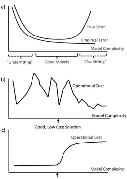
In the framework of statistical learning theory (e.g., Vapnik, 1998; Pollard, 1984; Anthony and Bartlett, 1999; Zhang, 2002), prediction ability of a class of models is guaranteed when the class has low “complexity,” where complexity is defined via covering numbers, VC (Vapnik-Chervonenkis) dimension, Rademacher complexity, gaussian complexity, etc. Limiting the complexity of the hy-pothesis space imposes a bias, and the classical image associated with the bias-variance tradeoff is provided in Figure 1(a). The set of good models is indicated on the axis of the figure. Models that are not good are either overfitted (explaining too much of the variance of the data, having a high complexity), or underfitted (having too strong of a bias and a high empirical error). By understand-ing complexity, we can find a model class where both the trainunderstand-ing error and the complexity are kept low. An example of increasingly complex model classes is the set of nested classes of polynomials, starting with constants, then linear functions, second order polynomials and so on.

Figure 1: In all three plots, the x-axis represents model classes with increasing complexity. a) Relationship between training error and test error as a function of model complexity. b) A possible operational cost as a function of model complexity. c) Another possible operational cost.

Recall that question Q3 asked if our intuition about how much it will cost to solve a problem can help us produce a better probabilistic model. Figure 1 can be used to illustrate how this question can be answered. Assume we have a strong prior belief that the operational cost will not be above a certain fixed amount.

bound on the complexity of the hypothesis space, thereby obtaining a better prediction guarantee for the simultaneous process than for the sequential process. In Section 5 we develop results of this type. These results indicate that in some cases, the operational cost can be an important quantity for generalization.

3. Conceptual Demonstrations

We provide four examples. In the first, we estimate manpower requirements for a scheduling task. In the second, we estimate real estate prices for a purchasing decision. In the third, we estimate call arrival rates for a call center staffing problem. In the fourth, we estimate failure probabilities for manholes (access points to an underground electrical grid). The first two are small scale repro-ducible examples, designed to demonstrate new types of constraints due to operational costs. In the first example, the operational cost subproblem involves scheduling. In the second, it is a knap-sack problem, and in the third, it is another multidimensional knapknap-sack variant. In the fourth, it is a routing problem. In the first, second and fourth examples, the operational cost leads to a linear constraint, while in the third example, the cost leads to a quadratic constraint.

Throughout this section, we will assume that we are working with linear functions fof the form

βT_{xso that Π(f,{x˜}

i}i)can be denoted byΠ(β,{x˜i}i). We will set R(f) to be equal tokβk22. We will also use the notation

F

R_{to denote the set of linear functions that satisfy an additional property:}

F

R:=_{f _∈

F

unc:R(f)_≤C₂∗_},

whereC∗₂is a known constant greater than zero. We will use constantC2from (1), and alsoC₂∗from the definition of

F

R_{, to control the extent of regularization. C}

2 is inversely related toC∗2. We use both versions interchangeably throughout the paper.

3.1 Manpower Data and Scheduling with Precedence Constraints

We aim to schedule the starting times of medical staff, who work at 6 stations, for instance, ultra-sound, X-ray, MRI, CT scan, nuclear imaging, and blood lab. Current and incoming patients need to go through some of these stations in a particular order. The six stations and the possible orders are shown in Figure 2. Each station is denoted by a line. Work starts at the check-in (at timeπ1) and ends at the check-out (at timeπ5). The stations are numbered 6-11, in order to avoid confusion with the timesπ1-π5. The clinic has precedence constraints, where a station cannot be staffed (or work with patients) until the preceding stations are likely to finish with their patients. For instance, the check-out should not start until all the previous stations finish. Also, as shown in Figure 2, station 11 should not start until stations 8 and 9 are complete at timeπ4, and station 9 should not start until station 7 is complete at timeπ3. Stations 8 and 10 should not start until station 6 is complete. (This is related to a similar problem calledplanning with preferenceposed by F. Malucelli, Politecnico di Milano).

The operational goal is to minimize the total time of the clinic’s operation, from when the check-in happens at timeπ1until the check-out happens at timeπ5. We estimate the time it takes for each station to finish its job with the patients based on two variables: the new load of patients for the day at the station, and the number of current patients already present. The data are available as

Figure 2: Staffing estimation with bias on scheduling with precedence constraints.

(βT_x

i) and the actual times it took to finish (yi). The unlabeled data are the new load and current patients present at each station for a given period, given as ˜x6, ..,x˜11. Letπdenote the 5-dimensional real vector with coordinatesπ1, ...,π5.

The operational cost is the total timeπ5−π1. Step 1, with an optimistic bias, can be written as: min

{β:kβk2 2≤C2∗}

n

∑

i=1

(yi−βTxi)2+C1 min

π_∈Π(β,{x˜i}i)

(π5−π1), (4)

where the feasible setΠ(β,_{x˜i}i)is defined by the following constraints:

πa+βTx˜i≤πb; (a,i,b)∈ {(1,6,2),(1,7,3),(2,8,4),(3,9,4),(2,10,5),(4,11,5)}

πa≥0 fora=1, ...,5.

To solve (4) given values ofC1andC2, we used a function-evaluation-based scheme called Nelder-Mead (Nelder and Nelder-Mead, 1965) where at every iterate of β, the subproblem for πwas solved to optimality (using Gurobi).1 _C

2was chosen heuristically based on (1) and kept fixed for the experi-ment beforehand.

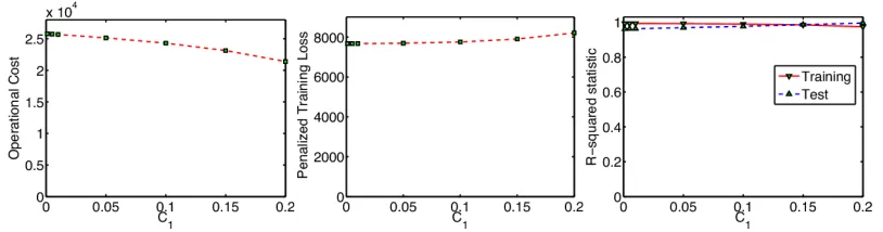
Figure 3 shows the operational cost, training loss, andr2statistic2for various values ofC1. For

C1values between 0 and 0.2, the operational cost varies substantially, by∼16%. Ther2values for both training and test vary much less, by_∼3.5%, where the best value happened to have the largest value ofC1. For small data sets, there is generally a variation between training and test: for this data split, there is a 3.16% difference inr2 between training and test for plain least squares, and this is similar across various splits of the training and test data. This means that for the scheduling problem, there is a range of reasonable predictive models within about_∼3.5% of each other.

What we learn from this, in terms of the three questions in the introduction, is that: 1) There is a wide range of possible costs within the range of reasonable optimistic models. 2) We have found a reasonable scenario, supported by data, where the cost is 16% lower than in the sequential case.

1. Gurobi is the Gurobi Optimizer v3.0 from Gurobi Optimization, Inc. 2010.

2. If ˆyiare the predicted labels and ¯yis the mean of{y1, ...,yn}, then the value of ther2statistic is defined as 1−∑i(yi−

ˆ

yi)2/∑i(yi−y¯)2. Thusr2is an affine transformation of the sum of squares error.r2allows training and test accuracy

Figure 3: Left: Operational cost vsC1. Center: Penalized training loss vsC1. Right: R-squared statistic.C1=0 corresponds to the baseline, which is the sequential formulation.

3) If we have a prior belief that the cost will be lower, the models that are more accurate are the ones with lower costs, and therefore we may not want to designate the full cost suggested by the sequential process. We can perhaps designate up to 16% less.

Connection to learning theory: In the experiment, we used tradeoff parameterC1 to provide a soft constraint. Considering instead the corresponding hard constraint minπ(π5−π1)≤α, the total time must be at least the time for any of the three paths in Figure 2, and thus at least the average of them:

α_≥ min

π∈Π{β,{x˜i}i}

π5−π1

≥max_{(x˜6+x˜10)Tβ,(x˜6+x˜8+x˜11)Tβ,(x˜7+x˜9+x˜11)Tβ}

≥zTβ (5)

where

z=1

3[(x˜6+x˜10) + (x˜6+x˜8+x˜11) + (x˜7+x˜9+x˜11)].

The main result in Section 5, Theorem 6, is a learning theoretic guarantee in the presence of this kind of arbitrary linear constraint,zTβ_≤α.

3.2 Housing Prices and the Knapsack Problem

A developer will purchase 3 properties amongst the 6 that are currently for sale and in addition, will remodel them. She wants to maximize the total value of the houses she picks (the value of a property is its purchase cost plus the fixed remodeling cost). The fixed remodeling costs for the 6 properties are denoted_{ci}6_i=1. She estimates the purchase cost of each property from data regarding historical sales, in this case, from theBoston Housing data set (Bache and Lichman, 2013), which has 13 features. Let policyπ_{∈ {}0,1_}6_{be the 6-dimensional binary vector that indicates the properties she} purchases. Also, xi represents the features of propertyiin the training data and ˜xi represents the features of a different property that is currently on sale. The training loss is chosen to be the sum of squares error between the estimated pricesβT_x

(mixed-integer) program for Step 1 of the simultaneous process is:

min

β∈{β:β∈R13_,kβk2 2≤C∗2}

n

∑

i=1

(yi−βTxi)2

+C1 "

max

π∈{0,1}6 6

∑

i=1

(βT_x˜

i+ci)πi subject to 6

∑

i=1

πi≤3

#

. (6)

Notice that the second term above is a 1-dimensional_{0,1_}knapsack instance. Since the set of policiesΠdoes not depend onβ, we can rewrite (6) in a cleaner way that was not possible directly with (4):

min

β maxπ

"

n

∑

i=1

(yi−βTxi)2+C1 6

∑

i=1

(βT_x˜

i+ci)πi

#

subject to

β_{∈ {}β:β_∈R13,_kβ_k2_2≤C₂∗_}

π_∈

(

π:π_{∈ {}0,1_}6, 6

∑

i=1

πi≤3

)

. (7)

To solve (7) with user-defined parametersC1andC2, we use fminimax, available through Mat-lab’s Optimization toolbox.3

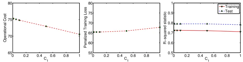
For the training and unlabeled set we chose, there is a change in policy above and belowC1= 0.05, where different properties are purchased. Figure 4 shows the operational cost which is the predicted total value of the houses after remodeling, the training loss, andr2values for a range of

C1. The training loss and r2 values change by less than ∼3.5%, whereas the total value changes about 6.5%. We can again draw conclusions in terms of the questions in the introduction as follows. The pessimistic bias shows that even if the developer chose the best response policy to the prices, she might end up with the expected total value of the purchased properties on the order of 6.5% less if she is unlucky. Also, we can now produce a realistic model where the total value is 6.5% less. We can use this model to help her understand the uncertainty involved in her investment.

Before moving to the next application of the proposed framework, we provide a bound analo-gous to that of (5). Let us replace the soft constraint represented by the second term of (6) with a hard constraint and then obtain a lower bound:

α_≥ max

π_∈{0,1_}6_,∑6

i=1πi≤3

6

∑

i=1

(βT_x˜ i)πi≥

6

∑

i=1

(βT_x˜

i)π′i, (8)

whereπ′ _{is some feasible solution of the linear programming relaxation of this problem that also} gives a lower objective value. For instance pickingπ′_i=0.5 fori=1, . . . ,6 is a valid lower bound giving us a looser constraint. The constraint can be rewritten:

βT 1

2 n

∑

i=1 ˜

xi

! ≤α.

0 0.2 0.4 0.6 0.8 1 0.5

0.6 0.7 0.8 0.9 1

C₁

R−squared statistic

Training Test

Figure 4: Left:Operational cost (total value) vsC1.Center:Penalized training loss vsC1.Right: R-squared statistic.C1=0 corresponds to the baseline, which is the sequential formulation.

This is again a linear constraint on the function class parametrized byβ, which we can use for the analysis in Section 5.

Note that if all six properties were being purchased by the developer instead of three, the knap-sack problem would have a trivial solution and the regularization term would be explicit (rather than implicit).

3.3 A Call Center’s Workload Estimation and Staff Scheduling

A call center management wants to come up with the per-half-hour schedule for the staff for a given day between 10am to 10pm. The staff on duty should be enough to meet the demand based on call arrival estimatesN(i),i=1, ...,24. The staff required will depend linearly on the demand per half-hour. The demand per half-hour in turn will be computed based on the Erlang C model (Aldor-Noiman et al., 2009) which is also known as the square-root staffing rule. This particular model relates the demandD(i)to the call arrival rateN(i)in the following manner:D(i)∝N(i) +cpN(i)

wherecdetermines where on the QED (Quality Efficiency Driven) curve the center wants to operate on. We make the simplifying assumptions that the service time for each customer is constant, and that the coefficientcis 0.

If we know the call arrival rateN(i), we can calculate the staffing requirements during each half hour. If we do not know the call arrival rate, we can estimate it from past data, and make optimistic or pessimistic staffing allocations.

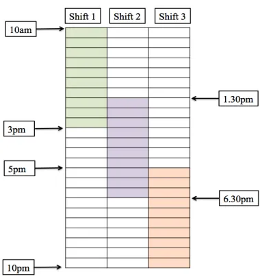
There are additional staffing constraints as shown in Figure 5, namely, there are three sets of employees who work at the center such that: the first set can work only from 10am-3pm, the second can work from 1:30pm-6:30pm, and the third set works from 5pm-10pm. The operational cost is the total number of employees hired to work that day (times a constant, which is the amount each person is paid). The objective of the management is to reduce the number of staff on duty but at the same time maintain a certain quality and efficiency.

Figure 5: The three shifts for the call center. The cells represent half-hour periods, and there are 24 periods per work day. Work starts at 10am and ends at 10pm.

Data for call arrivals and features were collected over a period of 10 months from Mid-February 2004 to the end of December 2004 (this is the same data set as in Aldor-Noiman et al., 2009). After converting categorical variables into binary encodings (e.g., each of the 7 weekdays into 6 binary features) the number of features is 36, and we randomly split the data into a training set and test set (2764 instances for training; another 3308 for test).

We now formalize the optimization problem for the simultaneous process. Let policy π_∈Z3+

be a size three vector indicating the number of employees for each of the three shifts. The training loss is the sum of squares error between the estimated square root of the arrival rateβT_x

i and the actual square root of the arrival rateyi:=

p

N(i). The cost is proportional to the total number of employees signed up to work,∑iπi. An optimistic bias on cost is chosen, so that the (mixed-integer) program for Step 1 is:

min

β:_kβ_k2 2≤C∗2

n

∑

i=1

(yi−βTxi)2

+C1 "

min

π

3

∑

i=1

πisubject toaTi π≥(βTx˜i)2fori=1, ...,24,π∈Z3+

#

, (9)

where Figure 5 illustrates the matrixAwith the shaded cells containing entry 1 and 0 elsewhere. The notationai indicates theithrow ofA:

ai(j) =

1 if staff jcan work in half-hour periodi

0 otherwise.

0 0.5 1 1.5 2 0

0.1 0.2 0.3 0.4 0.5 0.6

C₁

R−squared statistic

Training Test

Figure 6: Left: Operational cost vsC1. Center: Penalized training loss vsC1. Right: R-squared statistic.C1=0 corresponds to the baseline, which is the sequential formulation.

implementation of the Nelder-Mead algorithm, where at each step, Gurobi was used to solve the mixed-integer subproblem for finding the policy.

Figure 6 shows the operational cost, the training loss, and r2 values for a range of C1. The training loss andr2 values change only _∼1.6% and_∼3.9% respectively, whereas the operational cost changes about 9.2%. Similar to the previous two examples, we can again draw conclusions in terms of the questions in Section 1 as follows. The optimistic bias shows that the management might incur operational costs on the order of 9% less if they are lucky. Further, the simultaneous process produces a reasonable model where costs are about 9% less. If the management team believes they will be reasonably lucky, they can justify designating substantially less than the amount suggested by the traditional sequential process.

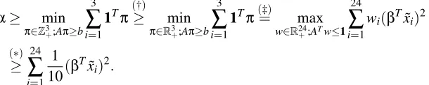
Let us now investigate the structure of the operational cost regularization term we have in (9). For convenience, let us stack the quantities(βT_x˜

i)2as a vectorb∈R24. Also let boldface symbol1 represent a vector of all ones. If we replace the soft constraint represented by the second term with a hard constraint having an upper boundα, we get:

α_≥ min

π∈Z3+;Aπ≥b

3

∑

i=1

1Tπ(_≥†) min

π∈R3+;Aπ≥b

3

∑

i=1

1Tπ(=‡) max w∈R24

+;ATw≤1

24

∑

i=1

wi(βTx˜i)2

(∗)

≥ 24

∑

i=1 1 10(β

T_x˜ i)2.

Hereα is related to the choice ofC1 and is fixed. (†) represents an LP relaxation of the integer program with π now belonging to the positive orthant rather than the cartesian product of set of positive integers.(‡)is due to LP strong duality and(_∗)is by choosing an appropriate feasible dual variable. Specifically, we pickwi=₁₀1 fori=1, . . . ,24, which is feasible because staff cannot work more than 10 half hour shifts (or 5 hours). With the three inequalities, we now have a constraint on

βof the form:

24

∑

i=1

(βT_x˜

i)2≤10α.

This is a quadratic form inβand gives an ellipsoidal feasible set. We already had a simple ellipsoidal feasibility constraint while defining the minimization problem of (9) of the form_kβ_k2

has become smaller. This in turn affects generalization. We are investigating generalization bounds for this type of hypothesis set in separate ongoing work.

3.4 The Machine Learning and Traveling Repairman Problem (ML&TRP) (Tulabandhula et al., 2011)

Recently, power companies have been investing in intelligent “proactive” maintenance for the power grid, in order to enhance public safety and reliability of electrical service. For instance, New York City has implemented new inspection and repair programs for manholes, where a manhole is an access point to the underground electrical system. Electrical grids can be extremely large (there are on the order of 23,000-53,000 manholes in each borough of NYC), and parts of the underground distribution network in many cities can be as old as 130 years, dating from the time of Thomas Edi-son. Because of the difficulties in collecting and analyzing historical electrical grid data, electrical grid repair and maintenance has been performed reactively (fix it only when it breaks), until recently (Urbina, 2004). These new proactive maintenance programs open the door for machine learning to assist with smart grid maintenance.

Machine learning models have started to be used for proactive maintenance in NYC, where supervised ranking algorithms are used to rank the manholes in order of predicted susceptibility to failure (fires, explosions, smoke) so that the most vulnerable manholes can be prioritized (Rudin et al., 2010, 2012, 2011). The machine learning algorithms make reasonably accurate predictions of manhole vulnerability; however, they do not (nor would they, using any other prediction-only technique) take the cost of repairs into account when making the ranked lists. They do not know that it is unreasonable, for example, if a repair crew has to travel across the city and back again for each manhole inspection, losing important time in the process. The power company must solve an optimization problem to determine the best repair route, based on the machine learning model’s output. We might wish to find a policy that is not only supported by the historical power grid data (that ranks more vulnerable manholes above less vulnerable ones), but also would give a better route for the repair crew. An algorithm that could find such a route would lead to an improvement in repair operations on NYC’s power grid, other power grids across the world, and improvements in many different kinds of routing operations (delivery trucks, trains, airplanes).

The simultaneous process could be used to solve this problem, where the operational cost is the price to route the repair crew along a graph, and the probabilities of failure at each node in the graph must be estimated. We call this the “the machine learning and traveling repairman problem” (ML&TRP) and in our ongoing work (Tulabandhula et al., 2011) , we have developed several for-mulations for the ML&TRP. We demonstrated, using manholes from the Bronx region of NYC, that it is possible to obtain a much more practical route using the ML&TRP, by taking the cost of the route optimistically into account in the machine learning model. We showed also that from the routing problem, we can obtain a linear constraint on the hypothesis space, in order to apply the generalization analysis of Section 5 (and in order to address question Q3 of Section 1).

4. Connections to Robust Optimization

The goal of robust optimization (RO) is to provide the best possible policy that is acceptable under a wide range of situations.4 _{This is different from the simultaneous process, which aims to find the}

best policies and costs for specific situations. Note that it is not always desirable to have a policy that is robust to a wide range of situations; this is a question of whether to respond to every situation simultaneously or whether to understand the single worst situation that could reasonably occur (which is what the pessimistic simultaneous formulation handles). In general, robust optimization can be overly pessimistic, requiring us to allocate enough to handle all reasonable situations; it can be substantially more pessimistic than the pessimistic simultaneous process.

In robust optimization, if there are several real-valued parameters involved in the optimization problem, we might declare a reasonable range, called the “uncertainty set,” for each parameter (e.g., a1 ∈[9,10], a2∈[1,2]). Using techniques of RO, we would minimize the largest possible operational cost that could arise from parameter settings in these ranges. Estimation is not usually involved in the study of robust optimization (with some exceptions, see Xu et al., 2009, who consider support vector machines). On the other hand, one could choose the uncertainty set according to a statistical model, which is how we will build a connection to RO. Here, we choose the uncertainty set to be the class of models that fit the data to withinε, according to some fitting criteria.

The major goals of the field of RO include algorithms, geometry, and tractability in finding the best policy, whereas our work is not concerned with finding a robust policy, but we are concerned with estimation, taking the policy into account. Tractability for us is not always a main concern as we need to be able to solve the optimization problem, even to use the sequential process. Using even a small optimization problem as the operational cost might have a large impact on the model and decision. If the unlabeled set is not too large, or if the policy optimization problem can be broken into smaller subproblems, there is no problem with tractability. An example where the policy optimization might be broken into smaller subproblems is when the policy involves routing several different vehicles, where each vehicle must visit part of the unlabeled set; in that case there is a small subproblem for each vehicle. On the other hand, even though the goals of the simultaneous process and RO are entirely different, there is a strong connection with respect to the formulations for the simultaneous process and RO, and a class of problems for which they are equivalent. We will explore this connection in this section.

There are other methods that consider uncertainty in optimization, though not via the lens of estimation and learning. In the simplest case, one can perform both local and global sensitivity analysis for linear programs to ascertain uncertainty in the optimal solution and objective, but these techniques generally only handle simple forms of uncertainty (Vanderbei, 2008). Our work is also related to stochastic programming, where the goal is to find a policy that is robust to almost all of the possible circumstances (rather than all of them), where there are random variables governing the parameters of the problem, with known distributions (Birge and Louveaux, 1997). Again, our goal is not to find a policy that is necessarily robust to (almost all of) the worst cases, and estimation is again not the primary concern for stochastic programming, rather it is how to take known randomness into account when determining the policy.

4.1 Equivalence Between RO and the Simultaneous Process in Some Cases

In Section 2, we had introduced the notation_{(xi,yi)}i and{x˜i}ifor labeled and unlabeled data respectively. We had also introduced the class

F

unc _{in which we were searching for a function f}∗ by minimizing an objective of the form (1). The uncertainty set

F

_goodwill turn out to be a subset of

F

unc_{that depends on{(x}

i,yi)}iand f∗but not on{x˜i}i.

We start with plain (non-robust) optimization, using a general version of the vanilla sequential process. Let fdenote an element of the set

F

_good, where f is pre-determined, known and fixed. Let the optimization problem for the policy decisionπbe defined by:

min

π∈Π(f;{x˜}i)

OpCost(π,f;{x˜i}), (Base problem) (10)

whereΠ(f;_{x˜i})is the feasible set for the optimization problem. Note that this is a more general version of the sequential process than in Section 2, since we have allowed the constraint setΠto be a function of both f and_{x˜i}i, whereas in (2) and (3), only the objective and not the constraint set can depend on f and_{x˜i}i. Allowing this more general version ofΠwill allow us to relate (10) to RO more clearly, and will help us to specify the additional assumptions we need in order to show the equivalence relationship. Specifically, in Section 2, OpCost depends on (f,_{x˜i}i) but not Π; whereas in RO, generallyΠdepends on(f,_{x˜i}i)but not OpCost. The fact that OpCost does not need to depend on f and_{x˜i}iis not a serious issue, since we can generally remove their dependence through auxiliary variables. For instance, if the problem is a minimization of the form (10), we can use an auxiliary variable, sayt, to obtain an equivalent problem:

min

π,t t (Base problem reformulated)

such thatπ_∈Π(f;_{x˜i}) OpCost(π,f;_{x˜i})≤t

where the dependence on(f,_{x˜i}i)is present only in the (new) feasible set. Since we had assumed f to be fixed, this is a deterministic optimization problem (convex, mixed-integer, nonlinear, etc.).

Now, consider the case when fis not known exactly but only known to lie in the uncertainty set

F

_good. The robust counterpart to (10) can then be written as:

min

π∈ ∩ g∈Fgood

Π(g;{x˜}i)

max f∈Fgood

OpCost(π,f;_{x˜i}) (Robust counterpart) (11)

where we obtain a “robustly feasible solution” that is guaranteed to remain feasible for all values of

f _∈

F

_good. In general, (11) is much harder to solve than (10) and is a topic of much interest in the robust optimization community. As we discussed earlier, there is no focus in (11) on estimation, but it is possible to embed an estimation problem within the description of the set

F

good, which we now define formally.

In Section 3,

F

R_{(a subset of}

_F

unc_{) was defined as the set of linear functionals with the property} thatR(f)_≤C₂∗. That is,

F

R=_{f :f _∈

F

unc,R(f)_≤C₂∗_}. We define

F

good as a subset of

F

Rby adding an additional property:

F

_good=

(

f : f_∈

F

R_,

_∑

n i=1

l(f(xi),yi)≤ n

∑

i=1

l(f∗(xi),yi) +ε

)

for some fixed positive realε. In (12), again f∗ is a solution that minimizes the objective in (1) over

F

unc_{. The right hand side of the inequality in (12) is thus constant, and we will henceforth} denote it with a single quantityC∗₁. Substituting this definition of

F

_good in (11), and further making an important assumption (denotedA1) thatΠis not a function of(f,_{x˜i}i), we get the following optimization problem:

min

π∈Π_{f∈FR_:∑nmax

i=1l(f(xi),yi)≤C1∗}

h

OpCost(π,f,_{x˜i}i)

i

(Robust counterpart with assumptions) (13)

whereC₁∗now controls the amount of the uncertainty via the set

F

_good.

Before we state the equivalence relationship, we restate the formulations for optimistic and pessimistic biases on operational cost in the simultaneous process from (2) and (3):

min f∈Func

"

n

∑

i=1

l(f(xi),yi) +C2R(f) +C1min

π∈ΠOpCost(π,f,{x˜i}i)

#

(Simultaneous optimistic),

min f∈Func

"

n

∑

i=1

l(f(xi),yi) +C2R(f)−C1min

π∈ΠOpCost(π,f,{x˜i}i)

#

(Simultaneous pessimistic). (14)

Apart from the assumptionA1on the decision setΠthat we made in (13), we will also assume that

F

gooddefined in (12) is convex; this will be assumptionA2. If we also assume that the objective OpCost satisfies some nice properties (A3), and that uncertainty is characterized via the set

F

_good, then we can show that the two problems, namely (14) and (13), are equivalent. Let _⇔ denote equivalence between two problems, meaning that a solution to one side translates into the solution of the other side for some parameter values (C1,C∗1,C2,C2∗).

Proposition 1 LetΠ(f;_{x˜i}i) =Πbe compact, convex, and independent of parameters f and{x˜i}i (assumptionA1). Let _{f _∈

F

R_:∑n

i=1l(f(xi),yi)≤C₁∗}be convex (assumptionA2). Let the cost (to be minimized)OpCost(π,f,_{x˜i}i)be concave continuous in f and convex continuous inπ (as-sumption A3). Then, the robust optimization problem (13) is equivalent to the pessimistic bias optimization problem (14). That is,

min

π_∈Π_{f∈FR_:∑nmax

i=1l(f(xi),yi)≤C1∗}

h

OpCost(π,f,_{x˜i}i)

i ⇔

min f∈Func

"

n

∑

i=1

l(f(xi),yi) +C2R(f)−C1min

π∈ΠOpCost(π,f,{x˜i}i)

# .

Remark 2 That the equivalence applies to linear programs (LPs) is clear because the objective is linear and the feasible set is generally a polyhedron, and is thus convex. For integer programs, the objective OpCost satisfies continuity, but the feasible set is typically not convex, and hence, the result does not generally apply to integer programs. In other words, the requirement that the constraint setΠbe convex excludes integer programs.

Definition 3 A linear topological space (also called a topological vector space) is a vector space over a topological field (typically, the real numbers with their standard topology) with a topology such that vector addition and scalar multiplication are continuous functions. For example, any normed vector space is a linear topological space. A function h is upper semicontinuous at a point p0 if for everyε>0there exists a neighborhood U of p0 such that h(p)≤h(p0) +εfor all

p_∈U . A function h defined over a convex set is quasi-concave if for all p,q andλ_∈[0,1] we have h(λp+ (1₋λ)q)_≥min(h(p),h(q)). Similar definitions follow for lower semicontinuity and quasi-convexity.

Theorem 4 (Sion’s minimax theorem Sion, 1958) LetΠ be a compact convex subset of a linear topological space and Ξbe a convex subset of a linear topological space. Let G(π,ξ)be a real function onΠ_×Ξsuch that

(i) G(π,_·)is upper semicontinuous and quasi-concave onΞfor eachπ_∈Π;

(ii) G(_·,ξ)is lower semicontinuous and quasi-convex onΠfor eachξ_∈Ξ. Then

min

π∈Πsup_ξ∈ΞG(π,ξ) =_ξsup_∈Ξminπ∈ΠG(π,ξ).

We can now proceed to the proof of Proposition (1).

Proof (Of Proposition 1)We start from the left hand side of the equivalence we want to prove:

min

π∈Π_{f∈FR_:∑nmax

i=1l(f(xi),yi)≤C∗1}

h

OpCost(π,f,_{x˜i}i)

i

(a)

⇔ max

{f∈FR_:∑n

i=1l(f(xi),yi)≤C∗1} min

π∈Π

h

OpCost(π,f,_{x˜i}i)

i

(b)

⇔ max f∈Func

h −_C1

1 n

∑

i=1

l(f(xi),yi)−C1∗

−C_C2 1

R(f)₋C₂∗

+min

π∈ΠOpCost(π,f,{x˜i}i)

i

(c)

⇔ min f∈Func

"

n

∑

i=1

l(f(xi),yi) +C2R(f)−C1min

π∈ΠOpCost(π,f,{x˜i}i)

# .

which is the right hand side of the logical equivalence in the statement of the theorem. In step

(a) we applied Sion’s minimax theorem (Theorem 4) which is satisfied because of the assump-tions we made. In step(b), we picked Lagrange coefficients, namely _C11 andC2_C1, both of which are positive. In particular,C₁∗andC1as well asC∗2andC2are related by the Lagrange relaxation equiv-alence (strong duality). In(c), we multiplied the objective withC1throughout, pulled the negative sign in front, and removed the constant termsC∗₁ andC2C∗2 and used the following observation: maxa−g(a) =−minag(a); and finally, removed the negative sign in front as this does not affect equivalence.

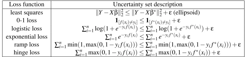
4.2 Creating Uncertainty Sets for RO Using Loss Functions from Machine Learning

Let us for simplicity specialize our loss function to the least squares loss. LetX be ann_×pmatrix with each training instancexi forming theith row. Also letY be then-dimensional vector of all the labelsyi. Then the loss term of (1) can be written as:

n

∑

i=1

(yi−f(xi))2= n

∑

i=1

(yi−βTxi)2=kY−Xβk22.

Letβ∗be a parameter corresponding to f∗in (1). Then the definition of

F

good in terms of the least squares loss is:

F

_good=_{f :f ∈

F

R_,kY−Xβk2

2≤ kY−Xβ∗k22+ε}={f :f ∈

F

R,kY−Xβk22≤C1∗}. Since each f _∈

F

good corresponds to at least oneβ, the optimization of (1) can be performed with respect to β. In particular, the constraint_kY₋Xβ_{k ≤}C∗₁ is an ellipsoid constraint onβ. For the purposes of the robust counterpart in (11), we can thus say that the uncertainty is of the ellipsoidal form. In fact, ellipsoidal constraints on uncertain parameters are widely used in robust optimization, especially because the resulting optimization problems often remain tractable.

Box constraints are also a popular way of incorporating uncertainty into robust optimization. For box constraints, the uncertainty over the p-dimensional parameter vector β= [β1, ...,βp]T is written fori=1, ...,pasLBi≤βi≤U Bi,where{LBi}iand{U Bi}iare real-valued upper and lower bounds that together define the box intervals.

Our main point in this subsection is that one can potentially derive a very wide range of un-certainty sets for robust optimization using different loss functions from machine learning. Box constraints and ellipsoidal constraints are two simple types of constraints that could potentially be the set

F

_good, which arise from two different loss functions, as we have shown. The least squares loss leads to ellipsoidal constraints on the uncertainty set, but it is unclear what the structure would be for uncertainty sets arising from the 0-1 loss, ramp loss, hinge loss, logistic loss and exponential loss among others. Further, it is possible to create a loss function for fitting data to a probabilistic model using the method of maximum likelihood; uncertainty sets for maximum likelihood could thus be established. Table 4.2 shows several different popular loss functions and the uncertainty sets they might lead to. Many of these new uncertainty sets do not always give tractable mathe-matical programs, which could explain why they are not commonly considered in the optimization literature.

The sequential process for RO.If we design the uncertainty sets as described above, with respect to a machine learning loss function, the sequential process described in Section 2 can be used with robust optimization. This proceeds in three steps:

1. use a learning algorithm on the training data to get f∗,

2. establish an uncertainty set based on the loss function and f∗, for example, ellipsoidal con-straints arising from the least squares loss (or one could use any of the new uncertainty sets discussed in the previous paragraph),

Loss function Uncertainty set description least squares _kY₋Xβ_k2

2≤ kY−Xβ∗k22+ε(ellipsoid) 0-1 loss 1_[f(xi)6=yi]≤1[f∗(xi)6=yi]+ε

logistic loss ∑n_i=1log(1+e−yif(xi)_)≤∑n

i=1log(1+e−yif

∗_(x i)_{) +ε}

exponential loss ∑n_i=1e−yif(xi)_≤∑n

i=1e−yif

∗_(x i)_+ε

ramp loss ∑n_i=1min(1,max(0,1₋yif(xi)))≤∑ni=1min(1,max(0,1−yif∗(xi))) +ε hinge loss ∑ni=1max(0,1−yif(xi))≤∑ni=1max(0,1−yif∗(xi)) +ε

Table 1: Table showing a summary of different possible uncertainty set descriptions that are based on ML loss functions.

We note that the uncertainty sets created by the 0-1 loss and ramp loss for instance, are non-convex, consequently assumption (A2) and Proposition 1 do not hold for robust optimization prob-lems that use these sets.

4.3 The Overlap Between The Simultaneous Process and RO

On the other end of the spectrum from robust optimization, one can think of “optimistic” optimiza-tion where we are seeking the best value of the objective in the best possible situaoptimiza-tion (as oppose to the worst possible situation in RO). For optimistic optimization, more uncertainty is favorable, and we find the best policy for the best possible situation. This could be useful in many real appli-cations where one not only wants to know the worst-case conservative policy but also the best case risk-taking policy. A typical formulation, following (11) can be written as:

min

π∈ ∪ g∈Fgood

Π(g;{x˜}i)

min f∈Fgood

OpCost(π,f;_{x˜i}). (Optimistic optimization)

In optimistic optimization, we view operational cost optimistically (minf∈FgoodOpCost) whereas in

the robust optimization counterpart (11), we view operational cost conservatively (maxf∈FgoodOpCost).

The policyπ∗_{is feasible in more situations in RO (minπ}

∈∩g∈F_goodΠ) since it must be feasible with

re-spect to each g_∈

F

_good, whereas the OpCost is lower in optimistic optimization (minπ∈∪g∈F_goodΠ)

since it need only be feasible with respect to at least one of theg’s. Optimistic optimization has not been heavily studied, possibly because a (min-min) formulation is relatively easier to solve than its (min-max) robust counterpart, and so is less computationally interesting. Also, one generally plans for the worst case more often than for the best case, particularly when no estimation is involved. In the case where estimation is involved, both optimistic and robust optimization could potentially be useful to a practitioner.

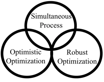
Figure 7: Set based description of the proposed framework (top circle) and its relation to robust (right circle) and optimistic (left circle) optimizations. The regions of intersection are where the conditions on the objective OpCost and the feasible setΠare satisfied.

problems. There is a class of problems that fall into the simultaneous process, but are not equivalent to robust or optimistic optimization problems. These are problems where we use operational cost to assist with estimation, as in the call center example and ML&TRP discussed in Section 3. Typically problems in this class have Π=Π(f;_{x˜i}i). This class includes problems where the bias can be either optimistic or pessimistic, and for whichFgoodhas a complicated structure, beyond ellipsoidal or box constraints. There are also problems contained in either robust optimization or optimistic optimization alone and do not belong to the simultaneous process. Typically, again, this is whenΠ

depends on f. Note that the housing problem presented in Section 3 lies within the intersection of optimistic optimization and the simultaneous process; this can be deduced from (7).

In Section 5, we will provide statistical guarantees for the simultaneous process. These are very different from the style of probabilistic guarantees in the robust optimization literature. There are some “sample complexity” bounds in the RO literature of the following form: how many observa-tions of uncertain data are required (and applied as simultaneous constraints) to maintain robustness of the solution with high probability? There is an unfortunate overlap in terminology; these are totally different problems to the sample complexity bounds in statistical learning theory. From the learning theory perspective, we ask: how many training instances does it take to come up with a modelβthat we reasonably know to be good? We will answer that question for a very general class of estimation problems.

5. Generalization Bound with New Linear Constraints

In this section, we give statistical learning theoretic results for the simultaneous process that involve counting integer points in convex bodies. Generalization bounds are probabilistic guarantees, that often depend on some measure of the complexity of the hypothesis space. Limiting the complexity of the hypothesis space equates to a better bound. In this section, we consider the complexity of hypothesis spaces that results from an operational cost bias.

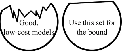
Figure 8: Left: hypothesis space for intersection of good models (circular, to represent ℓq ball) with low cost models (models below cost threshold, one side of wiggly curve). Right: relaxation to intersection of a half space with anℓqball.

Generalization bounds have been well established fornorm-basedconstraints on the hypothesis space, but the emphasis has been more on qualitative dependence (e.g., using big-O notation) and the constants are not emphasized. On the other hand, for a practitioner, every prior belief should reduce the number of examples they need to collect, as these examples may each be expensive to obtain; thus constants within the bounds, and even their approximate values, become important (Bousquet, 2003). We thus provide bounds on the covering number for new types of hypothesis spaces, emphasizing the role of constants.

To establish the bound, it is sufficient to provide an upper bound on the covering number. There are many existing generic generalization bounds in the literature (e.g., Bartlett and Mendelson, 2002), which combined with our bound, will yield a specific generalization bound for machine learning with operational costs, as we will construct in Theorem 10.

In Section 3, we showed that a bias on the operational cost can sometimes be transformed into linear constraints on model parameterβ(see Equations (5) and (8)). There is a broad class of other problems for which this is true, for example, for applications related to those presented in Section 3. Because we are able to obtain linear constraints for such a broad class of problems, we will analyze the case of linear constraints here. The hypothesis we consider is thus the intersection of anℓqball and a halfspace. This is illustrated in Figure 8.

The plan for the rest of the section is as follows. We will introduce the quantities on which our main result in this section depends. Then, we will state the main result (Theorem 6). Following that, we will build up to a generalization bound (Theorem 10) that incorporates Theorem 6. After that will be the proof of Theorem 6.

Definition 5 (Covering Number, Kolmogorov and Tikhomirov, 1959) Let A_⊆Γbe an arbitrary set and(Γ,ρ)a (pseudo-)metric space. Let_{| · |}denote set size.

• For anyε>0, anε-coverfor A is a finite set U _⊆Γ(not necessarily_⊆A) s.t._∀a_∈A,_∃u_∈U with dρ(a,u)≤ε.

• Thecovering numberof A is N(ε,A,ρ):=infU|U|where U is anε-cover for A.

soX can also be written as[h1···hp]. Define function class

F

as the set of linear functionals whose coefficients lie in anℓqball and with a set of linear constraints:

F

:=_{f :f(x) =βT_x,β

∈

B

_}where

B

:=

(

β_∈Rp:_kβ_kq≤Bb, p

∑

j=1

cjνβj+δν≤1,δν>0,ν=1, ...,V

) ,

where 1/r+1/q=1 and_{cjν}j,ν,{δν}νandBbare known constants. The linear constraints given by thecjν’s force the hypothesis space

F

to be smaller, which will help with generalization - this

will be shown formally by our main result in this section. Let

F

_|Sbe defined as the restriction of

F

with respect toS.

Let_{c˜jν}j,νbe proportional to{cjν}j,ν:

˜

cjν :=

cjνn1/rXbBb

khjkr ∀

j=1, ...,pandν=1, ...,V.

LetKbe a positive number. Further, let the setsPKparameterized byKandP_cKparameterized byK

and_{c˜jν}j,ν be defined as

PK:=

(

(k1, ...,kp)∈Zp: p

∑

j=1

|kj| ≤K

) .

P_cK:=

(

(k1, ...,kp)∈PK: p

∑

j=1 ˜

cjνkj≤K∀ν=1, ...,V

)

. (15)

Let_|PK_|and_|P_cK_|be the sizes of the setsPK andP_cK respectively. The subscriptcinP_cK denotes that this polyhedron is a constrained version ofPK. As the linear constraints given by thecjν’s

force the hypothesis space to be smaller, they force_|P_cK_|to be smaller. Define ˜X to be equal toX

times a diagonal matrix whose jthdiagonal element isn1/rXbBb

khjkr . Defineλmin(

˜

XTX˜)to be the smallest eigenvalue of the matrix ˜XT_{X˜, which will thus be non-negative. Using these definitions, we state} our main result of this section.

Theorem 6 (Main result, covering number bound)

N(√nε,

F

_|S,_{k · k}2)≤ (

min_{|PK0_|,_|P_cK_|} ifε<XbBb

1 otherwise , (16)

where

K0=

X_b2B2_b

ε2

and

K=max

  

 

K0, 

   

nX_b2B2_b

λmin(X˜TX˜) h

minν=1,...,V _∑pδν j=1|c˜jν|