CrossCat: A Fully Bayesian Nonparametric Method for Analyzing
Heterogeneous, High Dimensional Data
Vikash Mansinghka [email protected]
Patrick Shafto [email protected]
Eric Jonas [email protected]
Cap Petschulat [email protected]
Max Gasner [email protected]
Joshua B. Tenenbaum [email protected]
Editor:David Blei
Abstract
There is a widespread need for statistical methods that can analyze high-dimensional datasets with-out imposing restrictive or opaque modeling assumptions. This paper describes a domain-general data analysis method called CrossCat. CrossCat infers multiple non-overlapping views of the data, each consisting of a subset of the variables, and uses a separate nonparametric mixture to model each view. CrossCat is based on approximately Bayesian inference in a hierarchical, nonparamet-ric model for data tables. This model consists of a Dinonparamet-richlet process mixture over the columns of a data table in which each mixture component is itself an independent Dirichlet process mixture over the rows; the inner mixture components are simple parametric models whose form depends on the types of data in the table. CrossCat combines strengths of mixture modeling and Bayesian net-work structure learning. Like mixture modeling, CrossCat can model a broad class of distributions by positing latent variables, and produces representations that can be efficiently conditioned and sampled from for prediction. Like Bayesian networks, CrossCat represents the dependencies and independencies between variables, and thus remains accurate when there are multiple statistical signals. Inference is done via a scalable Gibbs sampling scheme; this paper shows that it works well in practice. This paper also includes empirical results on heterogeneous tabular data of up to 10 million cells, such as hospital cost and quality measures, voting records, unemployment rates, gene expression measurements, and images of handwritten digits. CrossCat infers structure that is consistent with accepted findings and common-sense knowledge in multiple domains and yields predictive accuracy competitive with generative, discriminative, and model-free alternatives.
Keywords: Bayesian nonparametrics, Dirichlet processes, Markov chain Monte Carlo, multivari-ate analysis, structure learning, unsupervised learning, semi-supervised learning
1. Introduction
This size and richness also enables the detection of subtle predictive relationships, including those that depend on aggregating individually weak signals from large numbers of variables. Challenges include integrating data of heterogeneous types (NRC Committee on the Analysis of Massive Data, 2013), suppressing spurious patterns (Benjamini and Hochberg, 1995; Attia, Ioannidis, et al., 2009), selecting features (Wasserman, 2011; Weston, Mukherjee, et al., 2001), and the prevalence of non-ignorable missing data.
This paper describes CrossCat, a general-purpose Bayesian method for analyzing high-dimens-ional mixed-type datasets that aims to mitigate these challenges. CrossCat is based on approximate inference in a hierarchical, nonparametric Bayesian model. This model is comprised of an “outer” Dirichlet process mixture over the columns of a table, with components that are themselves inde-pendent “inner” Dirichlet process mixture models over the rows. CrossCat is parameterized on a per-table basis by data type specific component models — for example, Beta-Bernoulli models for binary values and Normal-Gamma models for numerical values. Each “inner” mixture is solely re-sponsible for modeling a subset of the variables. Each hypothesis assumes a specific set of marginal dependencies and independencies. This formulation supports scalable algorithms for learning and prediction, specifically a collapsed MCMC scheme that marginalizes out all but the latent discrete state and hyper parameters.
The name “CrossCat” is derived from the combinatorial skeleton of this probabilistic model.
Each approximate posterior sample represents across-categorizationof the input data table. In a
cross-categorization, the variables are partitioned into a set ofviews, with a separate partition of the
entities into categorieswith respect to the variables in eachview. Each (category,variable) pair
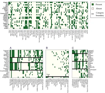
contains the sufficient statistics or latent state needed by its associated component model. See Fig-ure 1 for an illustration of this structFig-ure. From the standpoint of structFig-ure learning, CrossCat finds multiple, cross-cutting categorizations or clusterings of the data table. Each non-overlapping system of categories is context-sensitive in that it explains a different subset of the variables. Conditional densities are straightforward to calculate and to sample from. Doing so first requires dividing the conditioning and target variables into views, then sampling a category for each view. The distribu-tion on categories must reflect the values of the condidistribu-tioning variables. After choosing a category it is straightforward to sample predictions or evaluate predictive densities for each target variable by using the appropriate component model.
Standard approaches for inferring representations for joint distributions from data, such as Bayesian networks, mixture models, and sparse multivariate Gaussians, each exhibit complemen-tary strengths and limitations. Each method exhibits distinct strengths and weaknesses:
1. Bayesian networks and structure learning.
Present
Absent
Category boundary
A B C
the number of parameters to estimate (Elidan, Lotner, Friedman, and Koller, 2001; Elidan and Friedman, 2005). There are also computational difficulties. First, there are no known scalable techniques for fully Bayesian learning of Bayesian networks, so posterior uncertainty about the dependence structure is lost. Second, even when the training data is fully observed, i.e. all variables are observed, search through the space of networks is computationally demand-ing. Third, if the data is incomplete (or hidden variables are posited), a complex inference subproblem needs to be solved in the inner loop of structure search.
2. Parametric and semi-parametric mixture modeling.
Mixtures of simple parametric models have several appealing properties in this setting. First, they can accurately emulate the joint distribution within each group of variables by introduc-ing a sufficiently large number of mixture components. Second, heterogeneous data types are naturally handled using independent parametric models for each variable chosen based on the type of data it contains. Third, learning and prediction can both be done via MCMC techniques that are linear time per iteration, with constant factors and iteration counts that are often acceptable in practice. Unfortunately, mixture models assume that all variables are (marginally) coupled through the latent mixture component assignments. As a result, pos-terior samples will often contain good categorizations for one group of variables, but these same categories treat all other groups of mutually dependent variables as noise. This can lead to dramatic under-fitting in high dimensions or when missing values are frequent; this paper includes experiments illustrating this failure mode. Thus if the total number of variables is small enough, and the natural cluster structure of all groups of variables is sufficiently similar, and there is enough data, mixture models may perform well.
3. Multivariate Gaussians with sparse inverse covariances.
High-dimensional continuous distributions are often modeled as multivariate Gaussians with sparse conditional dependencies (Meinshausen and B¨uhlmann, 2006). Several parameter es-timation techniques are available; see e.g. (Friedman, Hastie, and Tibshirani, 2008). The pairwise dependencies produced by these methods form an undirected graph. The underlying assumptions are most appropriate when the number of variables and observations are suffi-ciently large, the data is naturally continuous and fully observed, and the joint distribution is approximately unimodal. A key advantage of these methods is the availability of fast algo-rithms for parameter estimation (though extensions for handling missing values require solv-ing challengsolv-ing non-convex optimization problems (St¨adler and B¨uhlmann, 2012)). These methods also have two main limitations. First, the assumption of joint Gaussianity is unreal-istic in many situations (Wasserman, 2011). Second, discrete values must be transformed into numerical values; this invalidates estimates of predictive uncertainty, and can generate other surprising behaviors.
(Dunson and Xing, 2009), and can emulate a broad class of generative processes and joint distri-butions given enough data. However, unlike mixture modeling but like Bayesian network structure learning, CrossCat can also detect independencies between variables. The “outer” Dirichlet process mixture partitions variables into groups that are independent of one another. As with estimation of sparse multivariate Gaussians (but unlike Bayesian network modeling), CrossCat can handle com-plex continuous distributions and report pairwise measures of association between variables. How-ever, in CrossCat, the couplings between variables can be nonlinear and heteroscedastic, and induce complex, multi-modal distributions. These statistical properties are illustrated using synthetic tests designed to strain the CrossCat modeling assumptions and inference algorithm.
This paper illustrates the flexibility of CrossCat by applying it to several exploratory analysis and predictive modeling tasks. Results on several real-world datasets of up to 10 million cells are described. Examples include measures of hospital cost and quality, voting records, US state-level unemployment time series, and handwritten digit images. These experiments show that CrossCat can extract latent structures that are consistent with accepted findings and common-sense knowledge in multiple domains. They also show that CrossCat can yield favorable predictive accuracy as compared to generative, discriminative, and model-free baselines.
The remainder of this paper is organized as follows. This section concludes with a discussion of related work. Section 2 focuses on generative model and approximate inference scheme behind CrossCat. Section 3 describes empirical results, and section 4 contains a broad discussion and summary of contributions.
1.1 Related Work
The observation that multiple alternative clusterings can often explain data better than a single clus-tering is not new to this paper. Methods for finding multiple clusclus-terings have been developed in several fields, including by the authors of this paper (see e.g. Niu, Dy, and Jordan, 2010; Cui, Fern, and Dy, 2007; Guan, Dy, Niu, and Ghahramani, 2010; Li and Shafto, 2011; Rodriguez and Ghosh, 2009; Shafto, Kemp, Mansinghka, Gordon, and Tenenbaum, 2006; Shafto, Kemp, Mansinghka, and Tenenbaum, 2011; Ross and Zemel, 2006). For example, Ross and Zemel (2006) used an EM approach to fit a parametric mixture of mixtures and applied it to image modeling. As nonpara-metric mixtures and model selection over finite mixtures can behave similarly, it might seem that a nonparametric formulation is a small modification. In fact, nonparametric formulation presented here is based on a super-exponentially larger space of model complexities that includes all possible numbers and sizes of views, and for each view, all possible numbers and sizes of categories. This expressiveness is necessary for the broad applicability of CrossCat. Cross-validation over this set is intractable, motivating the nonparametric formulation and sampling scheme used in this paper.
each atom on one Dirichlet process is associated with its own Dirichlet process, and inference is used to determine the number that will be expressed in a given finite dataset.
The nested Dirichlet process shares this combinatorial structure with CrossCat, but has been used to build very different statistical models. (Rodriguez et al., 2008) introduces it as a model for multiple related datasets. The model consists of a Dirichlet process mixture over datasets where each component is another Dirichlet process mixture models over the items in that dataset. From a statistical perspective, it can be helpful to think of this construction as follows. First, a top-level Dirichlet process is used to cluster datasets. Second, all datasets in the same cluster are pooled and their contents are modeled via a single clustering, provided by the lower-level Dirichlet process mixture model associated with that dataset cluster.
The differences between CrossCat and the nested Dirichlet process are clearest in terms of the nested Chinese restaurant process representation of the nested DP (Blei, Griffiths, Jordan, and Tenenbaum, 2004; Blei, Griffiths, and Jordan, 2010). In a 2-layer nested Chinese restaurant process, there is one customer per data vector. Each customer starts at the top level, sits a table at their current level according to a CRP, and descends to the CRP at the level below that the chosen table contains. In CrossCat, the top level CRP partitions the variables into views, and the lower level CRPs partition
the data vectors into categories for each view. If there areK tables in top CRP, i.e. the dataset is
divided into K views, then adding one datapoint leads to the seating ofK new customers at level
2. Each of these customers is deterministically assigned to a distinct table. Also, whenever a new
customer is created at the top restaurant, in addition to creating a new CRP at the level below, R
customers are immediately seated below it (one per row in the dataset).
Close relatives of CrossCat have been introduced by the authors of this paper in the cognitive science literature, and also by other authors in machine learning and statistics. This paper goes beyond this previous work in several ways. Guan et al. (2010) uses a variational algorithm for inference, while Rodriguez and Ghosh (2009) uses a sampler for the stick breaking representation for a Pitman-Yor (as opposed to Dirichlet Process) variant of the model. CrossCat is instead based on samplers that (i) operate over the combinatorial (i.e. Chinese restaurant) representation of the model, not the stick-breaking representation, and (ii) perform fully Bayesian inference over all hyper-parameters. This formulation leads to CrossCat’s scalability and robustness. This paper includes results on tables with millions of cells, without any parameter tuning, in contrast to the 148x500 gene expression subsample analyzed in Rodriguez and Ghosh (2009). These other papers include empirical results comparable in size to the authors’ experiments from Shafto et al. (2006) and Mansinghka, Jonas, Petschulat, Cronin, Shafto, and Tenenbaum (2009); these are 10-100x smaller than some of the examples from this paper. Additionally, all the previous work on variants of the CrossCat model focused on clustering, and did not articulate its use as a general model for high-dimensional data generators. For example, Guan et al. (2010) does not include predictions, although Rodriguez and Ghosh (2009) does discuss an example of imputation on a 51x26 table.
2. The CrossCat Model and Inference Algorithm
CrossCat is based on inference in a column-wise Dirichlet process mixture of Dirichlet process mixture models (Escobar and West, 1995; Rasmussen, 2000) over the rows. The “outer” or “column-wise” Dirichlet process mixture determines which dimensions/variables should be modeled together at all, and which should be modeled independently. The “inner” or “row-wise” mixtures are used to summarize the joint distribution of each group of dimensions/variables that are stochastically assigned to the same modeling subproblem.
This paper presents the Dirichlet processes in CrossCat via the convenient Chinese restaurant process representation (Pitman, 1996). Recall that the Dirichlet process is a stochastic process that maps an arbitrary underlying base measure into a measure over discrete atoms, where each atom is associated with a single draw from the base measure. In a set of repeated draws from this discrete measure, some atoms are likely to occur multiple times. In nonparametric Bayesian mixture modeling, each atom corresponds to a set of parameters for some mixture component; “popular” atoms correspond to mixture components with high weight. The Chinese restaurant process is a stochastic process that corresponds to the discrete residue of the Dirichlet process. It is sequential, easy to describe, easy to simulate, and exchangeable. It is often used to represent nonparametric mixture models as follows. Each data item is viewed as a customer at a restaurant with an infinite number of tables. Each table corresponds to a mixture component; the customers at each table thus comprise the groups of data that are modeled by the same mixture component. The choice
probabilities follow a simple “rich-gets-richer” scheme. Letmj be the number of customers (data
items) seated at a given table j, and zi be the table assignment of customeri(with the first table
z0 = 0), then the conditional probability distribution governing the Chinese restaurant process with
concentration parameterαis:
Pr(zi= j)∝
α if j=max(~z) +1 mj o.w.
This sequence of conditional probabilities induces a distribution over the partitions of the data that is equivalent to the marginal distribution on equivalence classes of atom assignments under the Dirichlet process. The Chinese restaurant process provides a simple but flexible modeling tool: the number of components in a mixture can be determined by the data, with support over all logically
possible clusterings. In CrossCat, thenumber of Chinese restaurant processes (over the rows) is
determined by the number of tables in a Chinese restaurant process over the columns. The data itself is modeled by datatype-specific component models for each dimension (column) of the target table.
2.1 The Generative Process
The generative process behind CrossCat unfolds in three steps:
1. Generating hyper-parameters and latent structure. First, the hyper-parameters~λd for
the component models for each dimension are chosen from a vague hyper-priorVd that is
appropriate1 for the type of data in d. Second, the concentration parameterα for the outer
Chinese restaurant process is sampled from a vague gamma hyper-prior. Third, a partition of
the variables into views,~z, is sampled from this outer Chinese restaurant process. Fourth, for
each view,v∈~z, a concentration parameterαvis sampled from a vague hyper-prior. Fifth, for
each viewv, a partition of the rows~yvis drawn using the appropriate inner Chinese restaurant
process with concentrationαv.
2. Generating category parameters for uncollapsed variables.This paper usesudas an
indi-cator of whether a given variable/dimensiond is uncollapsed (ud=1) or collapsed (ud=0).
For each uncollapsed variable, parametersθ~dc must be generated for each categorycfrom a
datatype-compatible prior modelMd.
3. Generating the observed data given hyper-parameters, latent structure, and parame-ters. The datasetX={x(r,d)} is generated separately for each variabled and for each
cat-egoryc∈~yv in the viewv=zd for that variable. For uncollapsed dimensions, this is done
by repeatedly simulating from a likelihood modelLd. For collapsed dimensions, we use an
exchangeably coupled modelMLd to generate all the data in each category at once.
The details of the CrossCat generative process are as follows:
1. GenerateαD, the concentration hyper-parameter for the Chinese Restaurant Process over
di-mensions, from a generic Gamma hyper-prior:αD∼Gamma(k=1,θ=1).
2. For each dimensiond∈D:
(a) Generate hyper-parameters~λd from a data type appropriate hyper-prior with density
p(~λd) =Vd(~λd), as described above. Binary data is handled by an asymmetric
Beta-Bernoulli model with pseudocounts~λd = [αd,βd]. Discrete data is handled by a
sym-metric Dirichlet-Discrete model with concentration parameterλd. Continuous data is
handled by a Normal-Gamma model with~λd = (µd,κd,υd,τd), where µd is the mean,
κd is the effective number of observations,υd is the degrees of freedom, andτd is the
sum of squares.
(b) Assign dimensiondto a viewzdfrom a Chinese Restaurant Process with concentration
hyper-parameterαD, conditional on all previous draws: zd∼CRP({z0,· · ·,zd−1};αD)
3. For each viewvin the dimension partition~z:
(a) Generateαv, the concentration hyper-parameter for the Chinese Restaurant Process over
categories in viewv, from a generic hyper-prior:αv∼Gamma(k=1,θ=1).
(b) For each observed data point (i.e. row of the table)r∈R, generate a category assignment
yvr from a Chinese Restaurant Process with concentration parameterαv, conditional on
all previous draws:yvr∼CRP({yv0,· · ·,yvr−1};αv)
apparent variation. Examples for strictly positive, real-valued hyper-parameters include vague Gamma(k=1,θ=1)
(c) For each categorycin the row partition for this view~yv:
i. For each dimensiondsuch thatud=1 (i.e. its component models are uncollapsed),
generate component model parametersθ~dc from the appropriate prior with density
Md(·;~λd)using hyper-parameters~λd, as follows:
A. For binary data, we have a scalarθdc equal to the probability that dimensiond
is equal to 1 for rows from category c, drawn from a Beta distribution: θdc ∼
Beta(αd,βd), where values from the hyper-parameter vector~λd= [αd,βd].
B. For categorical data, we have a vector-valuedθ~dc of probabilities, drawn from a
symmetric Dirichlet distribution with concentration parameter
λd:θ~dc ∼Dirichlet(λd).
C. For continuous data, we have θ~dc = (µdc,σdc), the mean and variance of the
data in the component, drawn from a Normal-Gamma distribution(µd
c,σdc)∼
NormalGamma(~λd).
ii. Let~xc(·,d)contain allx(r,d) in this component, i.e. forr such thatyzd
r =c. Generate
the data in this component, as follows:
A. Ifud =1, i.e. d is uncollapsed, then generate eachx(r,d)from the appropriate
likelihood model Ld(·;θ~dc). For binary data, we have x(r,d)∼Bernoulli(θdc);
for categorical data, we havex(r,d)∼Multinomial(θ~dc); for continuous data, we
havex(r,d)∼Normal(µdc,σdc).
B. Ifud=0, sodis collapsed, generate the entire contents of~xc(·,d)by directly
sim-ulating from the marginalized component model that with densityMLd(~x(·,d);~λd).
One approach is to sample from the sequence of predictive distributions
P(x(ri,d)|~x
−ri
(·,d).~λd), induced byMd andLd, indexing over rowsriin c.
The key steps in this process can be concisely described:
αD∼Gamma(k=1,θ=1)
~λd∼ Vd(·) foreachd∈ {1,· · ·,D}
zd∼ CRP({zi|i6=d};αD) foreachd∈ {1,· · ·,D}
αv∼ Gamma(k=1,θ=1) foreachv∈~z
yvr∼ CRP({yvi |i=6 r};αv) foreachv∈~zand
r∈ {1,· · ·,R}
~
θdc ∼ Md(·;~λd) foreachv∈~z,c∈~yv, anddsuch that
zd=vandud=1
~xc(·,d)={x(r,d)|yzrd =c} ∼ (
∏rLd(θ~dc) ifud=1
MLd(~λd) ifud=0
foreachv∈~zand eachc∈~yv
2.2 The Joint Probability Density
1. Vd(·), a generic hyper-prior of the appropriate type for variable/dimensiond.
2. {ud}, the indicators for which variables are uncollapsed.
3. Md(·)andLD(·)∀ds.t.ud=1, a datatype-appropriate parameter prior (e.g. a Beta prior for
binary data, Normal-Gamma for continuous data, or Dirichlet for discrete data) and likelihood model (e.g. Bernoulli, Normal or Multinomial).
4. MLd(·)∀d s.t.ud=0, a datatype-appropriate marginal likelihood model, e.g. the collapsed
version of the conjugate pair formed by someMdandLd.
5. Td({x}), the sufficient statistics for the component model for some collapsed dimensiond
from a subset of the data{x}. Arbitrary non-conjugate component models can be numerically
collapsed by choosingTd({x}) ={x}.
This paper will useCCto denote the information necessary to capture the dependence of
Cross-Cat on the dataX. This includes the view concentration parameterαD, the variable-specific
hyper-parameters {~λd}, the view partition~z, the view-specific concentration parameters {αv} and row
partition{~yv}, and the category-specific parameters{θd
c}or sufficient statisticsTd(~x(···,d)). This
pa-per will also overloadMLd,Md,Vd,Ld, andCRPto each represent both probability density functions
and stochastic simulators; the distinction should be clear based on context. Given this notation, we have:
P(CC,X) =P(X,{θ~dc},{~yv,αv},{~λd},~z,αD)
=e−αD
∏d∈DVd(~λd)
CRP(~z;αD) ∏v∈~ze−αvCRP(~yv;αv)
×
∏
v∈~z
∏
c∈~yvd∈{i
∏
s.t.zi=v}
(
MLd(Td(~xc(·,d));~λd) if ud=1
Md(~θdc;~λd)∏r∈cLd(x(r,d);θ~dc) ifud=0 !
2.3 Hypothesis Space and Modeling Capacity
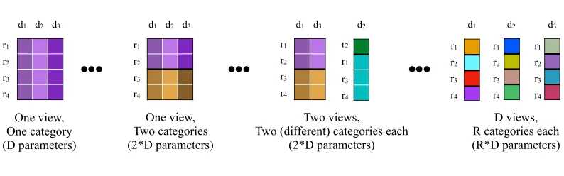
The modeling assumptions encoded in CrossCat are designed to enable it to emulate a broad class of data generators. One way to assess this class is to study the full hypothesis space of CrossCat, that is, all logically possible cross-categorizations. Figure 2 illustrates the version of this space that is induced by a 4 row, 3 column dataset. Each cross-categorization corresponds to a model structure — a set of dependence and independence assumptions — that is appropriate for some set of statistical situations. For example, conditioned on the hyper-parameters, the dependencies between variables and data values can be either dense or sparse. A group of dependencies will exhibit a unimodal joint distribution if they are modeled using only a single cluster. Strongly bimodal or multi-modal distributions as well as nearly unimodal distributions with some outliers are recovered by varying the number of clusters and their size. The prior favors stochastic relationships between groups of variables, but also supports (nearly) deterministic models; these correspond to structures with a large number of clusters that share low-entropy component models.
The CrossCat generative process favors hypotheses with multiple views and multiple categories
per view. A useful rule of thumb is to expectO(log(D))views withO(log(R))categories each a
r1 r2 r3 r4 r1 r2 r3 r4 r1 r2 r3 r4 r1 r2 r3 r4 r1 r2 r3 r4 r1 r2 r3 r4 r1 r2 r3 r4 One view, One category (D parameters) One view, Two categories (2*D parameters) Two views,
Two (different) categories each (2*D parameters)
D views, R categories each (R*D parameters)
d1 d2 d3 d1 d2 d3 d1 d3 d2 d1 d2 d3
Figure 2: Model structures drawn from the space of all logically possible cross-categorizations of a 4 row, 3 column dataset. In each structure, all data values (cells) that are governed by the same parametric model are shown in the same color. If two cells have different colors, they are modeled as conditionally independent given the model structure and hyper-parameters. In general, the space of all cross-categorizations contains a broad class of simple and complex data generators. See the main text for details.
single one. The second is that these processes cannot be summarized by a single parametric model, and thus induce non-Gaussian or multi-modal dependencies between the variables.
2.4 Posterior Inference Algorithm
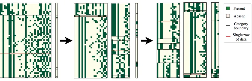
Posterior inference is carried out by simulating an ergodic Markov chain that converges to the pos-terior (Gilks, 1999; Neal, 1998). The state of the Markov chain is a data structure storing the cross-categorization, sufficient statistics, and all uncollapsed parameters and hyper-parameters. Figure 3 shows several sampled states from a typical run of the inference scheme on the dataset from Figure 1.
The CrossCat inference Markov chain initializes a candidate state by sampling it from the prior2
The transition operator that it iterates consists of an outer cycle of several kernels, each performing cycle sweeps that apply other transition operators to each segment of the latent state. The first is a
cycle kernel for inference over the outer CRP concentration parameterαand a cycle of kernels over
the inner CRP concentration parameters{αv}for each view. The second is a cycle of kernels for
inference over the hyper-parameters~λd for each dimension. The third is a kernel for inference over
any uncollapsed parameters~θdc. The fourth is a cycle over dimensions of an inter-view auxiliary
variable Gibbs kernel that shuffles dimensions between views. The fifth is itself a cycle over views of cycles that sweep a single-site Gibbs sampler over all the rows in the given view. This chain cor-responds to the default auxiliary variable Gibbs sampler that the Venture probabilistic programming platform (Mansinghka, Selsam, and Perov, 2014) produces when given the CrossCat model written as a probabilistic program.
More formally, the Markov chain used for inference is a cycle over the following kernels:
2. Anecdotally, this initialization appears to yield the best inference performance overall. One explanation can be found by considering a representative subproblem of inference in CrossCat: performing inference in one of the inner CRP mixture models. A maximally dispersed initialization, with each of theNrows in its own category, requiresO(N2)
Figure 3:Snapshots of the Markov chain for cross-categorization on a dataset of human object-feature judgments.Each of the three states shows a particular cross-categorization that arose during a single Markov chain run, automatically rendered using the latent structure from cross-categorization to inform the layout. Black horizontal lines separate categories within a view. The red horizontal line follows one row of the dataset. Taken from left to right, the three states span a typical run of roughly 100 iterations; the first is while the chain appears to be converging to a high probability region, while the last two illustrate variability within that region.
1. Concentration hyper-parameter inference: updatingαDand each element of{αv}.
Sam-pleαDand all theαvs for each view via a discretized Gibbs approximation to the posterior,
αD∼P(αD|~z)andαv∼P(αv|~yv). For eachα, this involves scoring the CRP marginal
like-lihood at a fixed number of grid points — typically∼100 — and then re-normalizing and
sampling from the resulting discrete approximation.
2. Component model hyper-parameter inference: updating the elements of {~λd}. For
each dimension, for each hyper-parameter, discretize the support of the hyper-prior and nu-merically sample from an approximate hyper-posterior distribution. That is, implement an
appropriately-binned discrete approximation to a Gibbs sampler for~λd∼P(~λd|~xd, ~yzd) (i.e.
we condition on the vertical slice of the input table described by the hyper-parameters, and the associated latent variables). For conjugate component models, the probabilities depend only on the sufficient statistics needed to evaluate this posterior. Each hyper-parameter ad-justment requires an operation linear in the number of categories, since the scores for each category (i.e. the marginal probabilities) must be recalculated, after each category’s statistics are updated. Thus each application of this kernel takes time proportional to the number of dimensions times the maximum number of categories in any view.
3. Category inference: updating the elements of{~yv}via Gibbs with auxiliary variables.
For each entity in each view, this transition operator samples a new category assignment from
its conditional posterior. A variant of Algorithm 8 from (Neal, 1998) (withm=1) is used to
handle uncollapsed dimensions.
The category inference transition operator will sampleyvr, the categorization for rowrin view
v, according to its conditioned distribution given the other category assignments~yv
−r,
param-eters{θ~dc}and auxiliary parameters. If ud =0 ∀d s.t.zd=v, i.e. there are no uncollapsed
the subset of data within the view. Otherwise, let{~φd}denote auxiliary parameters for each
uncollapsed dimensiond(whereud=1) of the same form asθ~dc. Before each transition, these
parameters are chosen as follows:
~φd∼
δθ~d
yvr
ifyvr=yvj ⇐⇒ r= j
Md(~λd) o.w.(yvr∈~yv−r)
In this section,c+will denote the category associated with the auxiliary variable. Ifyvr∈~yv−r,
thenc+=max(~yv−r) +1, i.e. a wholly new category will be created, and by sampling~φdthis
category will have newly sampled parameters. Otherwise,c+=yvr, i.e. rowrwas a singleton,
so its previous category assignment and parameters will be reused.
Given the auxiliary variables, we can derive the target density of the transition operator by expanding the joint probability density:
yvr∼P(yvr|~y v
−r,{~λd,{x(·,d)} |ds.t.zd=v},{{θ~dc |c∈~y
v
−r} |ds.t.zd=vandud=1},{~φd})
∝CRP(yvr;~yv−r,αv)
×
∏
d∈{is.t.zi=v}
MLd(Td(~xc(·,d)),~λd) ifud=0
Md(~θdc;~λd)∏r∈cLd(x(r,d);θ~dc) ifud=1 andyvr∈~yv−r
Md(~φdc;~λd)∏r∈cLd(x(r,d);φ~dc) ifud=1 andyvr=c+∈/~yv−r
The probabilities this transition operator needs can be obtained by iterating over possible
val-ues foryvr, calculating their joint densities, and re-normalizing numerically. These operations
can be implemented efficiently by maintaining and incrementally modifying a representation
ofCC, updating sufficient statistics and a joint probability accumulator after each change
(Mansinghka, 2007). The complexity of resamplingyvrfor all rowsrand viewsvisO(V RCD),
whereV is the number of views,Rthe number of rows,Cthe maximum number of categories
in any view, andDis the number of dimensions.
4. Inter-view inference: updating the elements of~zvia Gibbs with auxiliary variables. For
each dimension d, this transition operator samples a new view assignmentzd from its
con-ditional posterior. As with the category inference kernel, this can be viewed as a variant of
Algorithm 8 from (Neal, 1998) (withm=1), applied to the “outer” Dirichlet process mixture
model in CrossCat. This mixture has uncollapsed, non-conjugate component models that are themselves Dirichlet process mixtures.
Letv+be the index of the new view. The auxiliary variables areαv+,~yv
+
and{θd
c |c∈~yv
+
}
(ifud=1). Ifzd∈~z−d, thenv+=max(~z) +1, and the auxiliary variables are sampled from
their priors. Otherwise,v+=zd, and the auxiliary variables are deterministically set to the
values associated withzd. Given values for these variables, the conditional distribution forzd
can be derived as follows:
zd∼P(zd|αD,~λd,~z−d,αv+,{~yv},{{θdc |c∈~yzj} | j∈D},X)
∝CRP(zd;z~−d,αD)
∏
c∈~yzd(
MLd(Td(~xc(·,d)),~λd) if ud=1
This transition operator shuffles individual columns between views, weighing their compat-ibility with each view by multiplying likelihoods for each category. A full sweep thus has
time complexityO(DVCR). Note that if a given variable is a poor fit for its current view, its
hyper-parameters and parameters will be driven to reduce the dependence of the likelihood for that variable on its clustering. This makes it more likely for row categorizations proposed from the prior to be accepted.
Inference over the elements of~zcan also be done via a mixture of a Metropolis-Hastings
birth-death kernel to create new views with a standard Gibbs kernel to reassign dimensions among pre-existing views. In our experience, both transition operators yield comparable results on real-world data; the Gibbs auxiliary variable kernel is presented here for simplicity.
5. Component model parameter inference: updating{θ~dc |ud=1}. Each dimension or
vari-able whose component models are uncollapsed must be equipped with a suitvari-able ergodic
transition operatorT that converges to the local parameter posteriorP(θ~dc|x(c~·,d),~λd). Exact
Gibbs sampling is often possible whenLd andMdare conjugate.
CrossCat’s scalability can be assessed by multiplying an estimate of how long each transition takes with an estimate of how many transitions are needed to get good results. The experiments
in this paper use∼10-100 independent samples. Each sample was based on runs of the inference
Markov chain with∼100-1,000 transitions. Taking these numbers as rough constants, scalability is
governed by the asymptotic orders of growth. LetRbe the number of rows,Dthe number of
dimen-sions,V the maximum number of views andC the maximum number of categories. The memory
needed to store the latent state is the sum of the memory needed to store theDhyper-parameters
and view assignments, theVC parameters/sufficient statistics, and theV R category assignments,
orO(D+VC+V R). Assuming a fully dense data matrix, the loops in the transition operator
de-scribed above scale asO(DC+RDVC+RDVC+DC) =O(RDVC), with theRDterms scaling down
following the data density.
This paper shows results from both open-source and commercial implementations on datasets
of up to∼10 million cells3. Because this algorithm is asymptotically linear in runtime with low
memory requirements, a number of performance engineering and distributed techniques can be applied to reach larger scales at low latencies. Performance engineering details are beyond the scope of this paper.
2.5 Exploration and Prediction Using Posterior Samples
Each approximate posterior sample provides an estimate of the full joint distribution of the data. It also contains a candidate latent structure that characterizes the dependencies between variables and provides an independent clustering of the rows with respect to each group of dependent variables. This section gives examples of exploratory and predictive analysis problems that can be solved by using these samples. Prediction is based on calculating or sampling from the conditional densities implied by each sample and then either averaging or resampling from the results. Exploratory queries typically involve Monte Carlo estimation of posterior probabilities that assess structural
properties of the latent variables posited by CrossCat and the dependencies they imply. Examples include obtaining a global map of the pairwise dependencies between variables, selecting those variables that are probably predictive of some target, and identifying rows that are similar in light of some variables of interest.
2.5.1 PREDICTION
Recall thatCCrepresents a model for the joint distribution over the variables along with sufficient
statistics, parameters, a partition of variables into views, and categorizations of the rows in the data
X. Variables representing the latent structure associated with a particular posterior sample ˆCCswill
all be indexed bys, e.g. zsd. Also letYv+represent the category assignment of a new row in viewv,
and let{ti}and{gj}be the sets of target variables and given variables in a given predictive query.
To generate predictions by sampling from the conditional density on targets given the data, we must simulate
{xˆti} ∼p({Xti}|{Xgi=xgi},X)
Given a set of models, this can be done in two steps. First, from each model, sample a categorization from each view conditioned on the values of the given variables. Second, sample values for each target variable by simulating from the target variable’s component model for the sampled category:
ˆ
CCs∼p(CC|X)
csv∼p(Yv+|{Xgj =xgj|z
s gj=v})
ˆ
xts
i∼p(Xti|c
s zti) =
Z
L(xti;~θ
ti
cs
v)M(
~θti
cs
v;
~
λti)d~θ
The category kernel from the MCMC inference algorithm can be re-used to sample from csv.
Also, sampling from ˆxsti can be done directly given the sufficient statistics for data types whose
likelihood models and parameter priors are conjugate. In other cases, either~θwill be represented as
part of ˆCCsor sampled on demand.
The same latent variables are also useful for evaluating the conditional density for a desired set of predictions:
p({Xti=xti}|{Xgj =xgj},X)
≈ 1
N
∑
s p({Xti =xti}|{Xgj =xgj},CC=CCˆ s)= 1
N
∑
s v∏
∈~zs∑
cp({Xti =xti|z
s
gj =v}|Y
+
v =c)p(Yv+=c|{Xgj=xgj|z
s gj =v})
Many problems of prediction can be reduced to sampling from and/or calculating conditional densities. Examples include classification, regression and imputation. Each can be implemented
by forming estimates{Xt∗
i}of the target variables. By default, the implementation from this paper
equivalent to minimizing 0-1 loss, and calculates it by directly evaluating the conditional density of each possible value. This approach to prediction can also handle nonlinear and/or stochastic
relationships within the set of target variables{Xti}and between the given variables{Xgi}and the
targets. It is easy to implement in terms of the same sampling and probability calculation kernels that are necessary for inference.
This formulation of prediction scales linearly in the number of variables, categories, and view. It is also sub-linear in the number of variables when dependencies are sparse, and parallelizable over the views, the posterior samples, and the generated samples from the conditional density. Future work will explore the space of tradeoffs between accuracy, latency and throughput that can be achieved using this basic design.
2.5.2 DETECTINGDEPENDENCIESBETWEENVARIABLES
To detect dependencies between groups of variables, it is natural to use a Monte Carlo estimate of
the marginal posterior probability that a set of variables{qi}share the same posterior view. Using
sas a superscript to select values from a specific sample, we have:
Pr[zq0 =zq1=· · ·=zqk|X]≈
1
N
∑
s Pr[zs q0 =z
s
q1=· · ·=z
s qk|CCˆ s]
= #({s|z
s q0=z
s
q1=· · ·=z
s qk}) N
These probabilities also characterize the marginal dependencies and independencies that are
ex-plicitly represented by CrossCat. For example, pairwise co-assignment in~z determines4 pairwise
marginal independence under the generative model:
Xqi Xqj ⇐⇒ zqi6=zqk
The results in this paper often include the “z-matrix” of marginal dependence probabilities Z=
[Z(i,j)], whereZ(i,j)=1−Pr[Xi Xj|X]. This measure is used primarily for simplicity; other
mea-sures of the presence or strength of predictive relationships are possible.
2.5.3 ESTIMATINGSIMILARITYBETWEENROWS
Exploratory analyses often make use of “similarity” functions defined over pairs of rows. One use-ful measure of similarity is given by the probability that two pieces of data were generated from the same statistical model (Tenenbaum and Griffiths, 2001; Ghahramani and Heller, 2006). CrossCat naturally induces a context-sensitive similarity measure between rows that has this form: the prob-ability that two items come from the same category in some context. Here, contexts are defined by target variables, and comprise the set of views in which that variable participates (weighted by their probability). This probability is straightforward to estimate given a collection of samples:
1−Pr[x(r,c) x(r0,c)|X,~λc]≈
#({s|yzsc
(s,r)=y zs
c
(s,r0)})
N
This measure relies on CrossCat’s detection of marginal dependencies to determine which variables are relevant in any given context. The component models largely determine how differences in each variable in that view will be weighted when calculating similarity.
2.6 Assessing Inference Quality
A central concern is that the single-site Gibbs sampler used for inference might not produce high-quality models or stable posterior estimates within practical running times. For example, the Cross-Cat inference algorithm might rapidly converge to a local minimum in which all proposals to create new views are rejected. In this case, even though the Gibbs sampler will appear to have converged, the models it produces could yield poor inference quality.
This section reports four experiments that illustrate key algorithmic and statistical properties of CrossCat. The first experiment gives a rough sense of inference efficiency by comparing the energies of ground truth states to the energies of states sampled from CrossCat on data generated by the model. The second experiment assesses the convergence rate and the reliability of estimates of posterior expectations on a real-world dataset. The third experiment explores CrossCat’s resistance to under-fitting and over-fitting by running inference on datasets of Gaussian noise. The fourth experiment assesses CrossCat’s predictive accuracy in a setting with a large number of distractors and a small number of signal variables. It shows that CrossCat yields favorable accuracy compared to several baseline methods.
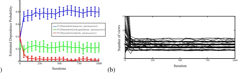
The next experiment assesses the stability and efficiency of CrossCat inference on real-world data. Figure 5a shows the evolution of Monte Carlo dependence probability estimates as a function of the number of Markov chain iterations. Figure 5b shows traces of the number of views for each
chain in the same set of runs. ∼100 iterations appears sufficient for initializations to be forgotten,
regardless of the number of views sampled from the CrossCat prior. At this point, Monte Carlo
esti-mates appear to stabilize, and the majority of states (∼40 of 50 total) appear to have 4, 5 or 6 views.
This stability is not simply due to a local minimum: after 700 iterations, transitions that create or destroy views are still being accepted. However, the frequency of these transitions does decrease. It thus seems likely that the standard MCMC approach of averaging over a single long chain run might require significantly more computation than parallel chains. This behavior is typical for ap-plications to real-world data. We typically use 10-100 chains, each run for 100-1,000 iterations, and have consistently obtained stable estimates.
The convergence measures from (Geweke, 1992) are also included for comparison, specifically the numerical standard error (NSE) and relative numerical efficiency (RNE) for the view CRP
pa-rameterα to assess autocorrelations (LeSage, 1999). NSE values near 0 and RNE values near 1
indicate approximately independent draws. These values were computed using a 0%, 4%, 8%, and
15% autocorrelation taper. NSE values were near zero and did not differ markedly: .023, .021,
.018, and.018. Similarly, RSE values were near 1 and did not differ markedly: 1, 1.23, 1.66, and
1.54. These results suggest that there is acceptably low autocorrelation in the sampled values of the
hyper-parameters.
One posterior sample Ground truth
Infe
rred l
ogs
core
Ground truth logscore
20000
0
20000
40000
60000
80000
100000
120000
140000
-15000 -10000 -5000 0 5000
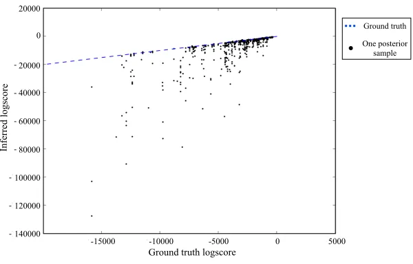
Figure 4:The joint density of the latent cross-categorization and training data for∼1,000 samples from CrossCat’s inference algorithm, compared to ground truth. Each point corresponds to a sample drawn from an approximation of the CrossCat posterior distribution after 200 iterations on data from a randomly chosen CrossCat model. Table sizes range from 10x10 to 512x512. Points on the blue line correspond to samples with the same joint density as the ground truth state. Points lying above the line correspond to models that most likely underestimate the entropy of the underlying generator, i.e. they have over-fit the data. CrossCat rarely produces such samples. Some points lie significantly below the line, overestimating the entropy of the generator. These do not necessarily correspond to “under-fit” models, as the true posterior will be broad (and may also induce broad predictions) when data is scarce.
uses independent samples from parallel chains, each initialized with an independent sample from the CrossCat prior. In contrast, typical MCMC schemes from nonparametric Bayesian statistics use dependent samples obtained by thinning a single long chain that was deterministically initialized. For example, Gibbs samplers for Dirichlet process mixtures are often initialized to a state with a sin-gle cluster; this corresponds to a sinsin-gle-view sinsin-gle-category state for CrossCat. Second, CrossCat performs inference over hyper-parameters that control the expected predictability of each dimen-sion, as well as the concentration parameters of all Dirichlet processes. Many machine learning applications of nonparametric Bayes do not include inference over these hyper-parameters; instead, they are set via cross-validation or other heuristics.
(a)
0 250 500 750 1000
0 0.2 0.4 0.6 0.8 1 Iterations E st im at ed D epe nde nc e P roba bi li ty
P r(Dependent(ami score, pneum score)) P r(Dependent(mcdr spnd home, pneum score)) P r(Dependent(snf beds, pneum score))
(b)
0 250 500 750 1000
0 5 10 15 N um be
r of vi
ew
s
Iteration
Figure 5: A quantitative assessment of the convergence rate of CrossCat inference and the stability of posterior estimates on a real-world health economics dataset. (a) shows the evolution of simple Monte Carlo estimates of the probability of dependence of three pairs of variables, made from independent chains initialized from the prior, as a function of the number of iterations of inference. Thick error bars show the standard deviation of estimates across 50 repetitions, each with 20 samples; thin lines show the standard deviation of estimates from 40 samples. Estimates stabilize after∼100 iterations. (b) shows the number of views for 50 of the same Markov chain runs. After∼100 iterations, states with 4, 5 or 6 views dominate the sample, and chains still can switch into and out of this region after 700 iterations.
by the categorization in its current view. Conditioned on such a categorization, the posterior on the hyper-parameter will favor increasing the expected noisiness of the clusters, to better accommodate the data. Once the hyper-parameter enters this regime, the model becomes less sensitive to the specific clustering used to explain this dimension. This therefore also increases the probability that the dimension will be reassigned to any other pre-existing view. It also increases the acceptance probability for proposals that create a new view with a random categorization. Once a satisfactory categorization is found, however, the Bayesian Occam’s Razor favors reducing the expected entropy of the clusters. Similar dynamics were described in (Mansinghka, Kulkarni, Perov, and Tenenbaum, 2013); a detailed study is beyond the scope of this paper.
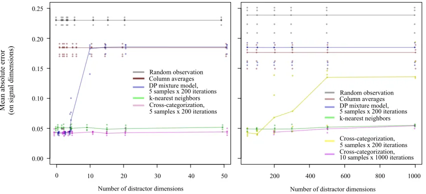
The third simulation, shown in Figure 7, illustrates CrossCat’s behavior on datasets with low-dimensional signals amidst high-low-dimensional random noise. In each case, CrossCat rapidly and confidently detects the independence between the “distractor” dimensions, i.e. it does not over-fit. Also, when the signal is strong or there are few distractors, CrossCat confidently detects the true predictive relationships. As the signals become weaker, CrossCat’s confidence decreases, and varia-tion increases. These examples qualitatively support the use of CrossCat’s estimates of dependence probabilities as indicators of the presence or absence of predictive relationships. A quantitative char-acterization of CrossCat’s sensitivity and specificity, as a function of both sample size and strength of dependence, is beyond the scope of this paper.
tech-1.0 - Pr[Xi Xk|X]
for strong signal, many distractors
(ρ=0.7,D=20)
Moderate signal, few distractors
(ρ=0.5,D=8)
Moderate signal, many distractors
(ρ=0.5,D=20)
Weak signal, few distractors
(ρ=0.25,D=8)
Figure 6: Detected dependencies given two correlated signal variables and multiple independent dis-tractors. This experiment illustrates CrossCat’s sensitivity and specificity to pairwise relationships on mul-tivariate Gaussian datasets with 100 rows. In each dataset, two pairs of variables have nonzero correlation
200 400 600 800 1000 0.00 0.05 0.10 0.15 0.20 0.25
Imputation performance on synthetic data
Number of distractor dimensions
Mean absolute error on signal dimensions
Column averages k−Nearest neighbors Random observation Cross−categorization, 5x200 Dirichlet process mixture model, 5x200 Cross−categorization, 10x1000
0 10 20 30 40 50
0.00 0.05 0.10 0.15 0.20 0.25
Imputation performance on synthetic data
Number of distractor dimensions
Mean absolute error on signal dimensions
Column averages k−Nearest neighbors Random observation Cross−categorization, 5x200 Dirichlet process mixture model, 5x200
Number of distractor dimensions Number of distractor dimensions
0 10 20 30 40 50 200 400 600 800 1000
0.25 0.20 0.15 0.10 0.05 0.00 M ea n a bs ol ut e e rror (on s igna l di m ens ions ) Random observation Column averages DP mixture model, 5 samples x 200 iterations k-nearest neighbors Cross-categorization, 5 samples x 200 iterations
Random observation Column averages DP mixture model, 5 samples x 200 iterations k-nearest neighbors
Cross-categorization, 5 samples x 200 iterations Cross-categorization, 10 samples x 1000 iterations
Figure 7: Predictive accuracy for low-dimensional signals embedded in high-dimensional noise. The data generator contains 10 “signal” dimensions described by a 5-cluster model to which distractor dimensions described by an independent 3-cluster model have been appended. The left plot shows imputation accuracies for up to 50 distractor dimensions; the right shows accuracies for 50-1,000 distractors. CrossCat is compared to mixture models as well as multiple non-probabilistic baselines (column-wise averaging, imputing via a random value, and a state-of-the-art extension to k-nearest-neighbors). The accuracy of mixture modeling drops when the number of distractors D becomes comparable to the number of signal variables S, i.e. when D≈S. When D>S, the distractors get modeled instead of the signal. In contrast, CrossCat remains accurate when the number of distractors is 100 times larger than the number of signal variables. See main text for additional discussion.
nique (Hastie, Tibshirani, Sherlock, Eisen, Brown, and Botstein, 1999) — on problems with varying numbers of distractors. CrossCat remains accurate when the number of distractors is 100x larger than the number of signal variables. As expected, mixtures are effective in low dimensions, but in-accurate in high dimensions. When the number of distractors equals the number of signal variables, the mixture posterior grows bimodal, including one mode that treats the signal variables as noise. This mode dominates when the number of distractors increases further.
3. Empirical Results on Real-World Datasets
3.1 Dartmouth Atlas of Health Care
The Dartmouth Atlas of Health Care (Fisher, Goodman, Wennberg, and Bronner, 2011) is one output from a long-running effort to understand the efficiency and effectiveness of the US health
care system. The overall dataset covers∼4300 hospitals that can be aggregated into∼300
hospi-tal reporting regions. The extract analyzed here contains 74 variables that collectively describe a hospital’s capacity, quality of care, and cost structure. These variables contain information about multiple functional units of a hospital, such as the intensive care unit (ICU), its surgery department, and any hospice services it offers. For several of these units, the amount each hospital bills to a federal program called Medicare is also available. The continuous variables in this dataset range over multiple orders of magnitude. Specific examples include counts of patients, counts of beds, dollar amounts, percentages that are ratios of counts in the dataset, and numerical aggregates from survey instruments that assess quality of care.
Due to its broad coverage of hospitals and their key characteristics, this dataset illustrates some of the opportunities and challenges described by the NRC Committee on the Analysis of Massive Data (2013). For example, given the range of cost variables and quality surveys it contains, this data could be used to study the relationship between cost and quality of care. The credibility of any re-sulting inferences would rest partly on the comprehensiveness of the dataset in both rows (hospitals) and columns (variables). However, it can be difficult to establish the absence of meaningful pre-dictive relationships in high-dimensional data on purely empirical grounds. Many possible sets of predictors and forms of relationships need to be considered and rejected, without sacrificing either sensitivity or specificity. If the dataset had fewer variables, a negative finding would be easier to es-tablish, both statistically and computationally, as there are fewer possibilities to consider. However, such a negative finding would be less convincing.
The dependencies detected by CrossCat reflect accepted findings about health care that may be surprising. The inferred pairwise dependence probabilities, shown in Figure 8, depict strong evidence for a dissociation between cost and quality. Specifically, the variables in block A are
ag-gregated quality scores, for congestive heart failure (CHF SCORE), pneumonia (PNEUM SCORE), acute
myocardial infarction (AMI SCORE), and an overall quality metric (QUAL SCORE). The probability
that they depend on any other variable in the dataset is low. This finding has been reported con-sistently across multiple studies and distinct patient populations (Fisher, Goodman, Skinner, and Bronner, 2009). Partly due to its coverage in the popular press (Gawande, 2009), it also informed the design of performance-based funding provisions in the 2009 Affordable Care Act.
CrossCat identifies several other clear, coherent blocks of variables whose dependencies are broadly consistent with common sense. For example, Section B of Figure 8 shows that CrossCat has inferred probable dependencies between three variables that all measure hospice usage. The dependencies within Section C reflect the proposition that the presence of home health aides — often consisting of expensive equipment — and overall equipment spending are probably dependent.
The dark green bar forMDCR SPND AMBLNCwith the variables in section C is also intuitive: home
Figure 8: Dependencies between variables the Dartmouth Atlas data aggregated by hospital referral region.This figure shows the z-matrixZ= [Z(i,j)]of pairwise dependence probabilities, where darker green
Figure 10:Subset of a single posterior sample for the Dartmouth Health Atlas.These entities have been color-coded according to geography. Variables related to quality are independent of geography (left), but variables related to usage of services are related to geography (right). This is in accord with a key finding from Gawande (2009).
It has been proposed that regional differences explain variation in cost and capacity, but not quality of care (Gawande, 2009). This proposal can be explored using CrossCat by examining indi-vidual samples as well as the context-sensitive pairwise co-categorization probabilities (similarities) for hospitals. Figure 9 shows these probabilities in the context of time spent in the ICU. These prob-abilities yield hospital groups that often contain adjacent regions, consistent with the idea that local variation in training or technique diffusion may contribute significantly to costs. Figure 10 shows results for regions from four states, coloring regions from the same state with the same color, with white space separating categories in a given view. Variables probably dependent on usage lead to geographically consistent partitions, while variables that are probably dependent on quality do not. The models inferred by CrossCat can also be used to compare each value in the dataset with the values that are probable given the rest of the data. Figure 11 shows the predictive distribution on the number of physician visits for ICU patients for 10 hospital reporting regions. The true values are relatively probable for most of these regions. However, for McAllen, Texas, the observed value is highly improbable. McAllen is known for having exceptionally high costs and an unusually large dependence on expensive, equipment-based treatment rather than physician care. In fact, Gawande (2009) used McAllen to illustrate how significant the variation can be.
Predicted MD_VISIT_P_DCD
Relative Probability
0 5 10 15 20
40 60 80 100120
Columbia MO Evansville IN
40 60 80 100120
Harrisburg PA Joliet IL
Little Rock AR McAllen TX Monroe LA
0 5 10 15 20 San Mateo County CA 0
5 10 15 20
Springfield MO
40 60 80 100120
Topeka KS
San Mateo CA
27
M
ea
n a
bs
ol
ut
e e
rror
5 10 15 20
0.0
0.2
0.4
0.6
0.8
1.0
Imputation performance on Dartmouth Atlas of Health
Percent of values missing
Mean absolute error
Column averages k−Nearest neighbors Random observation Cross−categorization, 10x1000 Dirichlet process mixture model, 10x1000
5
10
15
20
0.0
0.2
0.4
0.6
0.8
1.0
Percent of values missing
Mean absolute error
Column averages k−Nearest neighbors Random observation Cross−categorization, 10x1000 Dirichlet process mixture model, 10x1000
Column averages
k-nearest neighbors
Random observation Cross-categorization, 10 samples x1000 iterations DP mixture model, 10 samples x1000 iterations
0.0
0.2
0.4
0.6
0.8
1.0
Percent of values missing
5
10
15
20
3.2 Classifying Images of Handwritten Digits
The MNIST collection of handwritten digit images (LeCun and Cortes, 2011) can be used to ex-plore CrossCat’s applicability to high-dimensional prediction problems from pattern recognition. Figure 13a shows example digits. For all experiments, each image was downsampled to 16x16 pix-els and represented as a 256-dimensional binary vector. The digit label was treated as an additional categorical variable, observed for training examples and treated as missing for testing. Figure 13b shows the inferred dependence probabilities among pixels and between the digit label and the pix-els. The pixels that are identified as independent of the digit class label lie on the boundary of the image, as shown in Figure 13c.
A set of approximate posterior samples from CrossCat can be used to complete partially ob-served images by sampling predictions for arbitrary subsets of pixels. Figure 14 illustrates this: each panel shows the data, marginal predictive images, and predicted image completions, for 10 images from the dataset, one per digit. With no data, all 10 predictive distributions are equivalent, but as additional pixels are observed, the predictions for most images concentrate on representations
of the correct digit. Some digits remain ambiguous when∼30% of the pixels have been observed.
The predictive distributions begin as highly multi-modal distributions when there is little to no data, but concentrate on roughly unimodal distributions given sufficiently many features.
(a) (b) X130 X130 X146 X146 X114 X114 X98 X98 X82 X82 X66 X66 X36 X36 X51 X51 X53 X53 X52 X52 X85 X85 X84 X84 X68 X68 X69 X69 X99 X99 X83 X83 X67 X67 X222 X222 X206 X206 X204 X204 X205 X205 X221 X221 X220 X220 X238 X238 X236 X236 X237 X237 X189 X189 X190 X190 X188 X188 X187 X187 X219 X219 X203 X203 X86 X86 X70 X70 X100 X100 X101 X101 X163 X163 X124 X124 X125 X125 X131 X131 X147 X147 X149 X149 X148 X148 X133 X133 X132 X132 X117 X117 X116 X116 X115 X115 X158 X158 X126 X126 X142 X142 X157 X157 X141 X141 X140 X140 X156 X156 X174 X174 X173 X173 X172 X172 X111 X111 X107 X107 X110 X110 X108 X108 X109 X109 X95 X95 X79 X79 X94 X94 X78 X78 X77 X77 X76 X76 X93 X93 X92 X92 X62 X62 X60 X60 X61 X61 X179 X179 X211 X211 X195 X195 X212 X212 X213 X213 X197 X197 X196 X196 X210 X210 X194 X194 X178 X178 X162 X162 X250 X250 X234 X234 X251 X251 X183 X183 X230 X230 X231 X231 X215 X215 X199 X199 X232 X232 X233 X233 X216 X216 X217 X217 X201 X201 X200 X200 X184 X184 X185 X185 X235 X235 X186 X186 X218 X218 X202 X202 X23 X23 X227 X227 X229 X229 X228 X228 X245 X245 X244 X244 X106 X106 X166 X166 digit digit X122 X122 X123 X123 X120 X120 X121 X121 X119 X119 X167 X167 X138 X138 X154 X154 X134 X134 X150 X150 X136 X136 X135 X135 X151 X151 X137 X137 X153 X153 X152 X152 X171 X171 X168 X168 X170 X170 X169 X169 X118 X118 X139 X139 X155 X155 X164 X164 X165 X165 X180 X180 X181 X181 X59 X59 X91 X91 X75 X75 X248 X248 X249 X249 X214 X214 X198 X198 X182 X182 X247 X247 X246 X246 X55 X55 X58 X58 X57 X57 X56 X56 X39 X39 X38 X38 X42 X42 X43 X43 X87 X87 X71 X71 X104 X104 X105 X105 X54 X54 X102 X102 X103 X103 X37 X37 X40 X40 X41 X41 X72 X72 X73 X73 X88 X88 X89 X89 X90 X90 X74 X74 X44 X44 X45 X45 X22 X22 X226 X226 X81 X81 X97 X97 X240 X240 X14 X14 X129 X129 X225 X225 X128 X128 X3 X3 X12 X12 X255 X255 X8 X8 X6 X6 X28 X28 X29 X29 X223 X223 X19 X19 X241 X241 X242 X242 X11 X11 X177 X177 X176 X176 X0 X0 X34 X34 X4 X4 X224 X224 X161 X161 X35 X35 X7 X7 X47 X47 X16 X16 X1 X1 X10 X10 X144 X144 X160 X160 X33 X33 X18 X18 X30 X30 X113 X113 X32 X32 X31 X31 X48 X48 X20 X20 X21 X21 X17 X17 X2 X2 X193 X193 X208 X208 X15 X15 X9 X9 X13 X13 X239 X239 X5 X5 X27 X27 X49 X49 X145 X145 X112 X112 X192 X192 X209 X209 X65 X65 X80 X80 X64 X64 X50 X50 X96 X96 X26 X26 X24 X24 X25 X25 X127 X127 X175 X175 X143 X143 X159 X159 X254 X254 X207 X207 X46 X46 X243 X243 X63 X63 X191 X191 X252 X252 X253 X253(c)
30% observed All pixels
missing
Observed pixels {xi,j}obs (missing pixels
in turquoise)
Marginal predictive distribution
P( {xi,j} = 1 | {xi,j}obs} Ten samples from the
predictive distribution
True Digit
0
1
2
3
4
5
6
7
8
9
10% observed 18% observed
{xi,j} ~ P( {xi,j} | {xi,j}obs}
3.3 Voting Records for the 111th Senate
Voters are often members of multiple issue-dependent coalitions. For example, US senators some-times vote according to party lines, and at other some-times vote according to regional interests. Because this common-sense structure is typical for the CrossCat prior, voting records are an important test case.
This set of experiments describes the results of a CrossCat analysis of the 397 votes held by the 111th Senate during the 2009-2010 session. In this dataset, each column is a vote or bill, and each row is a senator. Figure 16 shows the raw voting data, with several votes and senators highlighted. There are 106 senators; this is senators is larger than the size of the senate by 6, due to deaths, replacement appointments, party switches, and special elections. When a senator did not vote on a given issue, that datum is treated as missing. Figure 16 also includes two posterior samples, one that reflects partisan alignment and another that posits a higher-resolution model for the votes.
This kind of structure is also apparent in estimates that aggregate across samples. Dependence probabilities between votes are shown in Figure 17. The visible independencies between blocks are compatible with a common-sense understanding of US politics. The two votes in orange are partisan issues. The two votes in green have broad bipartisan support. The vote in yellow aimed at removing an energy subsidy for rural areas, an issue that cross-cuts party lines. The vote in purple stipulates that the Department of Homeland Security must spend its funding through competitive processes, with an exception for small businesses and women or minority-owned businesses. This issue subdivides the republican party, isolating many of the most fiscally conservative. Similarity matrices for the senators with respect to S. 160 (orange) and an amendment to H.R. 2997 (yellow) are shown in Figure 18, with the senators whose similarity values changed the most between these two bills highlighted in grey.
It is instructive to compare the latent structure and predictions inferred by CrossCat with struc-tures and predictions from other learning techniques. As an individual voting record can be de-scribed by 397 binary variables and the missing values are negligible, Bayesian network structure learning is a suitable benchmark. Figure 19a shows the best Bayesian network structure found by structure learning using the search-and-score method implemented in the Bayes Net Toolbox for MATLAB (Murphy, 2001). This search is based on local moves similar to the transition operators from Giudici and Green (1999). The highest scoring graphs after 500 iterations contained between 143 and 193 links. Figure 19b shows the marginal dependencies between votes induced by this Bayesian network; these are sparser than those from CrossCat. Figure 19c shows the mean absolute errors for this Bayes net and for CrossCat on a predictive test where 25% of the votes were held out and predicted for senators in the test set. Bayes net CPTs were estimated using a symmetric
Beta-Bernoulli model with hyper-parameterα=1. CrossCat predictions were based on four samples,
Figure 18: Context-sensitive similarity measures for senators with respect to partisan and special-interest issues. The left matrix shows senator similarity for S. 181, the Lilly Ledbetter Fair Pay Act of 2009, a bill whose senator clusters tend to respect party lines. The right matrix is for H.R. 2997, a bill de-signed to remove a subsidy for energy generation systems in rural areas. The grey senators are those whose similarities changed the most between these two bills.
(a) (b) (c) 0 CrossCat BNT
0.1 0.2 0.3 0.4 0.5 0.6
Mean Absolute Error
CrossCat Bayes Net
M
ea
n
A
bs
ol
ut
e E
rror
0.6 0.5 0.4 0.3 0.2 0.1 0.0