Composite Binary Losses
Mark D. Reid∗ [email protected]
Robert C. Williamson∗ [email protected]
School of Computer Science, Building 108 Australian National University
Canberra ACT 0200, Australia
Editor: Rocco Servedio
Abstract
We study losses for binary classification and class probability estimation and extend the under-standing of them from margin losses to general composite losses which are the composition of a proper loss with a link function. We characterise when margin losses can be proper composite losses, explicitly show how to determine a symmetric loss in full from half of one of its partial losses, introduce an intrinsic parametrisation of composite binary losses and give a complete char-acterisation of the relationship between proper losses and “classification calibrated” losses. We also consider the question of the “best” surrogate binary loss. We introduce a precise notion of “best” and show there exist situations where two convex surrogate losses are incommensurable. We pro-vide a complete explicit characterisation of the convexity of composite binary losses in terms of the link function and the weight function associated with the proper loss which make up the com-posite loss. This characterisation suggests new ways of “surrogate tuning” as well as providing an explicit characterisation of when Bregman divergences on the unit interval are convex in their second argument. Finally, in an appendix we present some new algorithm-independent results on the relationship between properness, convexity and robustness to misclassification noise for binary losses and show that all convex proper losses are non-robust to misclassification noise.
Keywords: surrogate loss, convexity, probability estimation, classification, Fisher consistency, classification-calibrated, regret bound, proper scoring rule, Bregman divergence, robustness, mis-classification noise
1. Introduction
A loss function is the means by which a learning algorithm’s performance is judged. A binary loss function is a loss for a supervised prediction problem where there are two possible labels associated with the examples. A composite loss is the composition of a proper loss (defined below) and a link function (also defined below). In this paper we study composite binary losses and develop a number of new characterisation results. Several of these results can be seen as an extension of the work by Buja et al. (2005) applied to an analysis of composite losses by Masnadi-Shirazi and Vasconcelos (2009).
Informally, proper losses are well-calibrated losses for class probability estimation, that is for the problem of not only predicting a binary classification label, but providing an estimate of the probability that an example will have a positive label. Link functions are often used to map the out-puts of a predictor to the interval[0,1]so that they can be interpreted as probabilities. Having such
probabilities is often important in applications, and there has been considerable interest in under-standing how to get accurate probability estimates (Platt, 2000; Gneiting and Raftery, 2007; Cohen and Goldszmidt, 2004) and understanding the implications of requiring loss functions provide good probability estimates (Bartlett and Tewari, 2007).
Much previous work in the machine learning literature has focussed on margin losses which in-trinsically treat positive and negative classes symmetrically. However it is now well understood how important it is to be able to deal with the non-symmetric case (Zellner, 1986; Elkan, 2001; Provost and Fawcett, 2001; Buja et al., 2005; Bach et al., 2006; Beygelzimer et al., 2008; Christoffersen and Diebold, 2009). A key goal of the present work is to consider composite losses in the general (non-symmetric) situation. Since our development is for completely general losses, we automati-cally cover non-symmetric losses. The generalised notion of classification calibration developed in §5 is intrinsically non-symmetric.
1.1 Overview and Contributions
We now provide an overview of the paper’s structure, highlighting the novel contributions and how they relate to existing work. Central to this work are the notions of a loss and its associated condi-tional and full risk. These are introduced and briefly discussed in §2.
In §3 we introduce losses for Class Probability Estimation (CPE), define some technical prop-erties of them, and present some structural results originally by Shuford et al. (1966) and Savage (1971) and recently studied in a machine learning context by Buja et al. (2005) and Masnadi-Shirazi and Vasconcelos (2009). The most important of these are Theorem 4 which gives a representation of proper losses in terms of its associated conditional Bayes risk function, and Theorem 1 which relates a proper loss’s partial losses to its “weight function”—the negative second derivative of the conditional Bayes risk (see Corollary 3). We use these to provide a novel characterisation of proper symmetric CPE losses. Specifically, Theorem 9 shows these losses are completely determined by the behaviour of one of its partial losses on half the unit interval.
Learning algorithms often make real-valued predictions that are not directly interpretable as probability estimates but require a link function which maps their output to the interval[0,1]. In §4 we define composite losses as the composition of a CPE loss and a link. The new contributions of this section are Theorem 10 which generalises Theorem 1 to composite losses, and Corollaries 12 and 14 which shows how requiring properness completely determines the link function for compos-ite and margin losses. We also introduce a natural and intrinsic parametrisation of proper composcompos-ite losses that is a generalisation of the weight function and show how it can be used to easily derive gradients for stochastic descent algorithms.
In §5 we generalise the notion of classification calibrated losses (as studied, for example, by Bartlett et al., 2006) so it applies to non-symmetric composite losses (i.e., not just margin losses) and provide a characterisation of it in Theorem 17. We also describe how this new notion of clas-sification calibrated relates to proper CPE and composite losses via its connection with the weight function.
In §7 we study how the above insights can be applied to the problem of choosing a surrogate loss. Here, a surrogate loss function is a loss function which is not exactly what one wishes to minimise but is easier to work with algorithmically. This is still a relatively new area of research and our aim here is to open up a discussion rather than have the final word. To do so we define a well founded notion of “best” surrogate loss and show that some convex surrogate losses are incommensurable on some problems. We also consider some other notions of “best” and explicitly determine the surrogate loss that has the best surrogate regret bound in a certain sense.
Finally, in §8 we draw some more general conclusions. In particular, we argue that the weight and link function parametrisation of losses provides a convenient way to work with an entire class of losses that are central to probability estimation and may provide new ways of approaching the problem of “surrogate tuning” (Nock and Nielsen, 2009b).
Appendix C collects several observations which build upon some of the results in the main paper but are digressions from its central themes. In it, we present some new algorithm-independent results on the relationship between properness, convexity and robustness to misclassification noise for binary losses and show that all convex proper losses are non-robust to misclassification noise.
2. Losses and Risks
We write x∧y :=min(x,y)andJpK=1 if p is true andJpK=0 otherwise.1 The generalised function δ(·)is defined byRabδ(x)f(x)dx= f(0)when f is continuous at 0 and a<0<b. Random variables are written in sans-serif font:X,Y.
Given a set of labels Y:={−1,1}and a set of prediction values Vwe will say a loss is any function2ℓ:Y×V→[0,∞). We interpret such a loss as giving a penaltyℓ(y,v)when predicting the value v when an observed label is y. We can always write an arbitrary loss in terms of its partial lossesℓ1:=ℓ(1,·)andℓ−1:=ℓ(−1,·)using
ℓ(y,v) =Jy=1Kℓ1(v) +Jy=−1Kℓ−1(v).
Our definition of a loss function covers all commonly used margin losses (i.e., those which can be expressed asℓ(y,v) =φ(yv)for some functionφ:R→[0,∞)) such as the 0-1 lossℓ(y,v) =Jyv< 0K, the hinge lossℓ(y,v) =max(1−yv,0), the logistic lossℓ(y,v) =log(1+eyv), and the exponential loss ℓ(y,v) =e−yvcommonly used in boosting. It also covers class probability estimation losses where the predicted values ˆη∈V= [0,1]are directly interpreted as probability estimates.3 We will use ˆηinstead of v as an argument to indicate losses for class probability estimation and use the shorthand CPE losses to distinguish them from general losses. For example, square loss has partial lossesℓ−1(ηˆ) =ηˆ2andℓ1(ηˆ) = (1−ηˆ)2, the log lossℓ−1(ηˆ) =log(1−ηˆ)andℓ1(ηˆ) =log(ηˆ), and the family of cost-weighted misclassification losses parametrised by c∈(0,1)is given by
ℓc(−1,ηˆ) =cJηˆ ≥cKandℓc(1,ηˆ) = (1−c)Jηˆ <cK. (1)
1. This is the Iverson bracket notation as recommended by Knuth (1992).
2. Restricting the output of a loss to[0,∞)is equivalent to assuming the loss has a lower bound and then translating its output.
2.1 Conditional and Full Risks
Suppose we have random examplesXwith associated labelsY∈ {−1,1}The joint distribution of
(X,Y)is denotedPand the marginal distribution ofXis denoted M. Let the observation conditional densityη(x):=Pr(Y=1|X=x). Thus one can specify an experiment by eitherPor(η,M).
If η∈[0,1]is the probability of observing the label y=1 the point-wise risk (or conditional risk) of the estimate v∈Vis defined as theη-average of the point-wise loss for v:
L(η,v):=EY∼η[ℓ(Y,v)] =ηℓ1(v) + (1−η)ℓ−1(v).
Here,Y∼ηis a shorthand for labels being drawn from a Bernoulli distribution with parameterη. Whenη:X→[0,1]is an observation-conditional density, taking the M-average of the point-wise risk gives the (full) risk of the estimator v, now interpreted as a function v :X→V:
L(η,v,M):=EX∼M[L(η(X),v(X))].
We sometimes writeL(v,P)forL(η,v,M)where (η,M)corresponds to the joint distributionP. We writeℓ, L andLfor the loss, point-wise and full risk throughout this paper. The Bayes risk is the minimal achievable value of the risk and is denoted
L(η,M):= inf
v∈VXL(η,v,M) =EX∼M[L(η(X))],
where
[0,1]∋η7→L(η):=inf
v∈VL(η,v) is the point-wise or conditional Bayes risk.
There has been increasing awareness of the importance of the conditional Bayes risk curve L(η)—also known as “generalized entropy” (Gr¨unwald and Dawid, 2004)—in the analysis of losses for probability estimation (Kalnishkan et al., 2004, 2007; Abernethy et al., 2009; Masnadi-Shirazi and Vasconcelos, 2009). Below we will see how it is effectively the curvature of L that determines much of the structure of these losses.
3. Losses for Class Probability Estimation
We begin by considering CPE losses, that is, functions ℓ:{−1,1} ×[0,1]→[0,∞) and briefly summarise a number of important existing structural results for proper losses—a large, natural class of losses for class probability estimation.
3.1 Proper, Fair, Definite and Regular Losses
There are a few properties of losses for probability estimation that we will require. If ˆηis to be interpreted as an estimate of the true positive class probabilityη(i.e., when y=1) then it is desirable to require that L(η,ηˆ)be minimised by ˆη=ηfor allη∈[0,1]. Losses that satisfy this constraint are said to be Fisher consistent and are known as proper losses (Buja et al., 2005; Gneiting and Raftery, 2007). That is, a proper lossℓsatisfies L(η) =L(η,η)for allη∈[0,1]. A strictly proper loss is a proper loss for which the minimiser of L(η,ηˆ)over ˆηis unique.
We will say a loss is fair whenever
That is, there is no loss incurred for perfect prediction. The main place fairness is relied upon is in the integral representation of Theorem 6 where it is used to get rid of some constants of integration. In order to explicitly construct losses from their associated “weight functions” as shown in Theo-rem 7, we will require that the loss be definite, that is, its point-wise Bayes risk for deterministic events (i.e.,η=0 orη=1) must be bounded from below:
L(0)>−∞,L(1)>−∞.
Since properness of a loss ensures L(η) =L(η,η)we see that a fair proper loss is necessarily definite since L(0,0) =ℓ−1(0) =0>−∞, and similarly for L(1,1). Conversely, if a proper loss is definite then the finite valuesℓ−1(0)andℓ1(1)can be subtracted fromℓ−1(·)andℓ1(·)to make it fair.
Finally, for Theorem 4 to hold at the endpoints of the unit interval, we require a loss to be regular;4that is,
lim
ηց0ηℓ1(η) =ηlimր1(1−η)ℓ−1(η) =0.
Intuitively, this condition ensures that making mistakes on events that never happen should not incur a penalty. In most of the situations we consider in the remainder of this paper will involve losses which are proper, fair, definite and regular.
3.2 The Structure of Proper Losses
A key result in the study of proper losses is originally due to Shuford et al. (1966) and Sta¨el von Holstein (1970) (confer Aczel and Pfanzagl, 1967) though our presentation follows that of Buja et al. (2005). The following theorem5 characterises proper losses for probability estimation via a constraint on the relationship between its partial losses.
Theorem 1 (Shuford et al.) Supposeℓ:{−1,1} ×[0,1]→Ris a loss and that its partial lossesℓ1 andℓ−1are both differentiable. Thenℓis a proper loss if and only if for all ˆη∈(0,1)
−ℓ′1(ηˆ)
1−ηˆ = ℓ′−1(ηˆ)
ˆ
η =w(ηˆ) (2)
for some weight function w :(0,1)→R+such thatRε1−εw(c)dc<∞for allε>0. The equalities in (2) should be interpreted in the distributional sense.
This simple characterisation of the structure of proper losses has a number of interesting impli-cations. Observe from (2) that ifℓis proper, givenℓ1we can determineℓ−1or vice versa. Also, the partial derivative of the conditional risk can be seen to be the product of a linear term and the weight function:
Corollary 2 Ifℓis a differentiable proper loss then for allη∈[0,1]
∂
∂ηˆL(η,ηˆ) = (1−η)ℓ
′
−1(ηˆ) +ηℓ′1(ηˆ) = (ηˆ−η)w(ηˆ). (3) Another corollary, observed by Buja et al. (2005), is that the weight function is related to the curva-ture of the conditional Bayes risk L.
Corollary 3 Let ℓ be a a twice differentiable6 proper loss with weight function w defined as in Equation (2). Then for all c∈(0,1)its conditional Bayes risk L satisfies
w(c) =−L′′(c).
One immediate consequence of this corollary is that the conditional Bayes risk for a proper loss is always concave. Along with an extra constraint, this gives another characterisation of proper losses (Savage, 1971; Reid and Williamson, 2009a).
Theorem 4 (Savage) A loss function ℓis proper if and only if its point-wise Bayes risk L(η) is concave and for eachη,ηˆ ∈(0,1)
L(η,ηˆ) =L(ηˆ) + (η−ηˆ)L′(ηˆ).
Furthermore ifℓis regular this characterisation also holds at the endpointsη,ηˆ ∈ {0,1}.
This link between loss and concave functions makes it easy to establish a connection, as Buja et al. (2005) do, between regret∆L(η,ηˆ):=L(η,ηˆ)−L(η)for proper losses and Bregman divergences. The latter are generalisations of distances and are defined in terms of convex functions. Specifi-cally, if f :S→Ris a convex function over some convex setS⊆Rnthen its associated Bregman divergence7is
Df(s,s0):= f(s)−f(s0)− hs−s0,∇f(s0)i
for any s,s0∈S, where∇f(s0)is the gradient of f at s0. By noting that overS= [0,1]we have ∇f =f′, these definitions lead immediately to the following corollary of Theorem 4.
Corollary 5 Ifℓis a proper loss then its regret is the Bregman divergence associated with f =−L. That is,
∆L(η,ηˆ) =D−L(η,ηˆ).
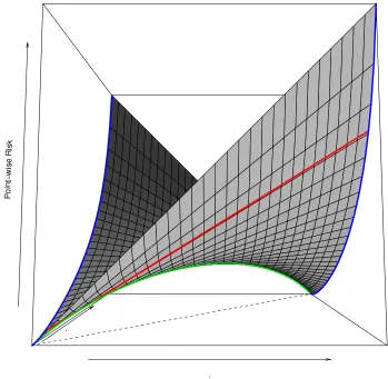
Many of the above results can be observed graphically by plotting the conditional risk for a proper loss as in Figure 1. Here we see the two partial losses on the left and right sides of the figure are related, for each fixed ˆη, by the linear mapη7→L(η,ηˆ) = (1−η)ℓ−1(ηˆ) +ηℓ1(ηˆ). For each fixedηthe properness ofℓrequires that these convex combinations of the partial losses (each slice parallel to the left and right faces) are minimised when ˆη=η. Thus, the lines joining the partial losses are tangent to the conditional Bayes risk curveη7→L(η) =L(η,η)shown above the dotted diagonal. Since the conditional Bayes risk curve is the lower envelope of these tangents it is necessarily concave. The coupling of the partial losses via the tangents to the conditional Bayes risk curve demonstrates why much of the structure of proper losses is determined by the curvature of L—that is, by the weight function w.
The relationship between a proper loss and its associated weight function is captured succinctly by Schervish (1989) via the following representation of proper losses as a weighted integral of the cost-weighted misclassification losses ℓc defined in (1). The reader is referred to Reid and
Williamson (2009b) for the details, proof and the history of this result.
6. The restriction to differentiable losses can be removed in most cases if generalised weight functions—that is, possibly infinite but defining a measure on(0,1)—are permitted. For example, the weight function for the 0-1 loss is w(c) =
δ(c−12).
Figure 1: The structure of the conditional risk L(η,ηˆ)for a proper loss (surface). The loss is log loss and its partialsℓ−1(ηˆ) =−log(ηˆ)andℓ1(ηˆ) =−log(1−ηˆ)shown on the left and right faces of the box. The conditional Bayes risk is the curve on the surface above the dotted line ˆη=η. The line connecting points on the partial loss curves shows the conditional risk for a fixed prediction ˆη.
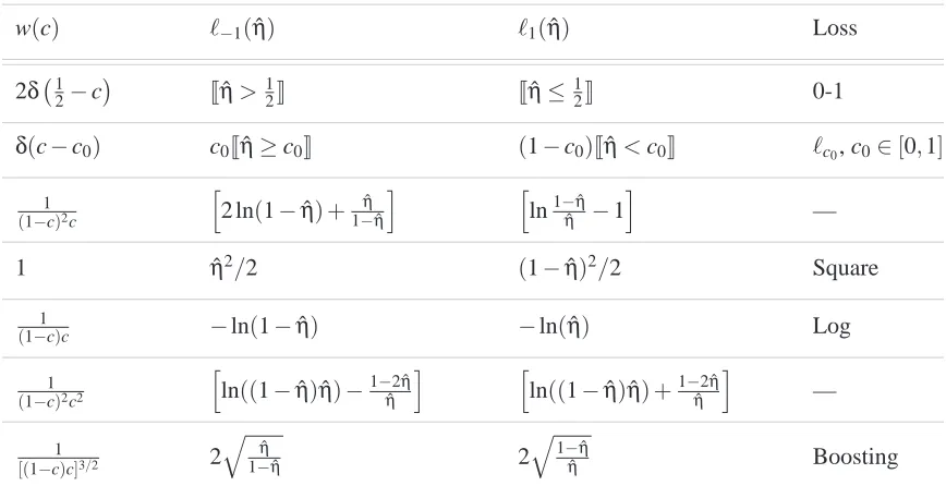
Theorem 6 (Schervish) Letℓ:Y×[0,1]→Rbe a fair, proper loss. Then for each ˆη∈(0,1)and y∈Y
ℓ(y,ηˆ) =
Z 1 0
ℓc(y,ηˆ)w(c)dc, (4)
where w=−L′′. Conversely, ifℓis defined by (4) for some weight function w :(0,1)→[0,∞)then it is proper.
w(c) ℓ−1(ηˆ) ℓ1(ηˆ) Loss 2δ 12−c Jηˆ >1
2K Jηˆ ≤
1
2K 0-1
δ(c−c0) c0Jηˆ ≥c0K (1−c0)Jηˆ <c0K ℓc0, c0∈[0,1]
1
(1−c)2c
h
2 ln(1−ηˆ) +1−ηˆηˆi hln1−ηˆηˆ −1i —
1 ηˆ2/2 (1−ηˆ)2/2 Square
1
(1−c)c −ln(1−ηˆ) −ln(ηˆ) Log
1
(1−c)2c2
h
ln((1−ηˆ)ηˆ)−1−ηˆ2 ˆηi hln((1−ηˆ)ηˆ) +1−ηˆ2 ˆηi — 1
[(1−c)c]3/2 2 q
ˆ η
1−ηˆ 2
q
1−ηˆ ˆ
η Boosting
Table 1: Weight functions and associated partial losses.
Theorem 7 (Reid and Williamson) Given a weight function w :[0,1]→[0,∞), let W(t) =Rtw(c)dc and W(t) =RtW(c)dc. Then the lossℓwdefined by
ℓw(y,ηˆ) =−W(ηˆ)−(y−ηˆ)W(ηˆ)
is a proper loss. Additionally, if W(0)and W(1)are both finite then
ℓw(y,ηˆ) + (W(1)−W(0))y+W(0)
is a fair, proper loss.
Observe that if w and v are weight functions which differ on a set of measure zero then they will lead to the same loss. A simple corollary to Theorem 6 is that the partial losses are given by
ℓ1(ηˆ) = Z 1
ˆ
η (1−c)w(c)dc and ℓ−1(ηˆ) = Z ηˆ
0
cw(c)dc. (5)
A similar8 integral representation of the partial losses can also be found in Shuford et al. (1966, Theorem 2) and Sta¨el von Holstein (1970).
3.3 Symmetric Losses
We will say a loss is symmetric ifℓ1(ηˆ) =ℓ−1(1−ηˆ) for all ˆη∈[0,1]. We say a weight function for a proper loss or the conditional Bayes risk is symmetric if w(c) =w(1−c)or L(c) =L(1−c)
for all c∈[0,1]. Perhaps unsurprisingly, an immediate consequence of Theorem 1 is that these two notions are identical.9
8. The weight function h in Theorem 2 of Shuford et al. (1966) is related to the w here by h(c) = (1−c)w(c). 9. The relationship between a symmetric L and symmetric behaviour of the loss has been previously recognised by
Corollary 8 A proper loss is symmetric if and only if its weight function is symmetric.
Proof If ℓ is symmetric, then ℓ′1(ηˆ) =−ℓ′−1(1−ηˆ) and so Equation (2) implies w(1−ηˆ) =
ℓ′−1(1−ηˆ)
1−ηˆ =
−ℓ′
1(ηˆ)
1−ηˆ =w(ηˆ). Conversely, the symmetry of w applied to Equation (5) establishes the symmetry ofℓ.
Requiring a loss to be proper and symmetric constrains the partial losses significantly. Proper-ness alone completely specifies one partial loss from the other. Now suppose in addition thatℓis symmetric. Combiningℓ1(ηˆ) =ℓ−1(1−ηˆ)with (2) implies
ℓ′−1(1−ηˆ) =1−ηˆ
ˆ
η ℓ′−1(ηˆ). (6)
This shows thatℓ−1is completely determined byℓ−1(ηˆ)for ˆη∈[0,12](or ˆη∈[12,1]). Thus in order to specify a symmetric proper loss, one needs to only specify one of the partial losses on one half of the interval[0,1]. Assumingℓ−1is continuous at 12 (or equivalently that w has no atoms at 12), by integrating both sides of (6) we can derive an explicit formula for the other half ofℓ−1in terms of that which is specified:
ℓ−1(ηˆ) =ℓ−1(12) + Z ηˆ
1 2
x 1−xℓ
′
−1(1−x)dx, (7)
which works for determiningℓ−1 on either[0,21]or[12,1]when ℓ−1 is specified on[12,1]or[0,12] respectively (recalling the usual convention thatRab=−Rba). We have thus shown:
Theorem 9 If a loss is proper and symmetric, then it is completely determined by specifying one of the partial losses on half the unit interval (either[0,1
2]or[ 1
2,0]) and using (6) and (7).
We demonstrate (7) with four examples. Suppose thatℓ−1(ηˆ) = 1−1ηˆ for ˆη∈[0,12]. Then one can readily determine the complete partial loss to be
ℓ−1(ηˆ) =
Jηˆ ≤1 2K
1−ηˆ +Jηˆ > 1 2K
2+log ηˆ 1−ηˆ
.
Suppose instead thatℓ−1(ηˆ) =1−1ηˆ for ˆη∈[12,1]. In that case we obtain
ℓ−1(ηˆ) =Jηˆ ≤ 1 2K
2+log ηˆ 1−ηˆ
+Jηˆ ≥
1 2K 1−ηˆ .
Supposeℓ−1(ηˆ) =(1−1ηˆ)2 for ˆη∈[0,12]. Then one can determine that
ℓ−1(ηˆ) =
Jηˆ <12K
(1−ηˆ)2+
Jηˆ ≥12K(4+2(2 ˆη+ηˆlog ˆη−ηˆlog(1−ηˆ)−1))
ˆ
η .
4. Composite Losses
General loss functions are often constructed with the aid of a link function. For a particular set of prediction valuesVthis is any continuous mappingψ: [0,1]→V. In this paper, our focus will be composite losses for binary class probability estimation. These are the composition of a CPE loss ℓ:{−1,1} ×[0,1]→Rand the inverse of a link functionψ, an invertible mapping from the unit interval to some range of values. Unless stated otherwise we will assumeψ:[0,1]→R. We will denote a composite loss by
ℓψ(y,v):=ℓ(y,ψ−1(v)). (8) The classical motivation for link functions (McCullagh and Nelder, 1989) is that often in estimating ηone uses a parametric representation of ˆη:X→[0,1] which has a natural scale not matching[0,1]. Traditionally one writes ˆη=ψ−1(ˆh)whereψ−1is the “inverse link” (andψis of course the forward link). The function ˆh :X→Ris the hypothesis. Often ˆh=ˆhαis parametrised linearly in a parameter
vectorα. In such a situation it is computationally convenient ifℓ(y,ψ−1(ˆh))is convex in ˆh (which implies it is convex inαwhen ˆhαis linear inα). The idea of a link function is not as well known as it should be and is thus reinvented—see for example Granger and Machina (2006).
Often one will choose the loss first (tailoring its properties by the weighting given according to w(c)), and then choose the link somewhat arbitrarily to map the hypotheses appropriately. An interesting alternative perspective arises in the literature on “elicitability”. Lambert et al. (2008)10 provide a general characterisation of proper scoring rules (i.e., losses) for general properties of distributions, that is, continuous and locally non-constant functionsΓwhich assign a real value to each distribution over a finite sample space. In the binary case, these properties provide another interpretation of links that is complementary to the usual one that treats the inverse linkψ−1 as a way of interpreting scores as class probabilities.
To see this, we first identify distributions over{−1,1}with the probabilityηof observing 1. In this case properties are continuous, locally non-constant mapsΓ:[0,1]→R. When a link function ψis continuous it can therefore be interpreted as a property since its assumed invertibility implies it is locally non-constant. A propertyΓis said to be elicitable whenever there exists a strictly proper lossℓfor it so that the composite lossℓΓsatisfies for all ˆη6=η
LΓ(η,ηˆ):=EY∼η[ℓΓ(Y,ηˆ)]>LΓ(η,η).
Theorem 1 of Lambert et al. (2008) shows thatΓis elicitable if and only ifΓ−1(r)is convex for all r∈range(Γ). This immediately gives us a characterisation of “proper” link functions: those that are both continuous and have convex level sets in[0,1]—they are the non-decreasing continuous functions. Thus in Lambert’s perspective, one chooses a “property” first (i.e., the invertible link) and then chooses the proper loss.
4.1 Proper Composite Losses
We will call a composite lossℓψ (8) a proper composite loss if ℓin (8) is a proper loss for class probability estimation. As in the case for losses for probability estimation, the requirement that a composite loss be proper imposes some constraints on its partial losses. Many of the results for proper losses carry over to composite losses with some extra factors to account for the link function.
Theorem 10 Letλ=ℓψ be a composite loss with differentiable and strictly monotone linkψand suppose the partial lossesλ−1(v)andλ1(v)are both differentiable. Thenλis a proper composite loss if and only if there exists a weight function w :(0,1)→R+ such that for all ˆη∈(0,1)
−λ′1(ψ(ηˆ))
1−ηˆ = λ′
−1(ψ(ηˆ)) ˆ
η =
w(ηˆ)
ψ′(ηˆ) =:ρ(ηˆ), (9)
where equality is interpreted in the distributional sense. Furthermore,ρ(ηˆ)≥0 for all ˆη∈(0,1).
Proof This is a direct consequence of Theorem 1 for proper losses for probability estimation and the chain rule applied toℓy(ηˆ) =λy(ψ(ηˆ)). Sinceψis assumed to be strictly monotonic we know ψ′>0 and so, since w≥0 we haveρ≥0.
As we shall see, the ratioρ(ηˆ)is a key quantity in the analysis of proper composite losses. For example, Corollary 2 has natural analogue in terms ofρthat will be of use later. It is obtained by letting ˆη=ψ−1(v)and using the chain rule.
Corollary 11 Supposeℓψis a proper composite loss with conditional risk denoted Lψ. Then ∂
∂vL
ψ(η,v) = (ψ−1(v)−η)ρ(ψ−1(v)). (10)
Loosely speaking then,ρis a “co-ordinate free” weight function for composite losses where the link functionψis interpreted as a mapping from arbitrary v∈Vto values which can be interpreted as probabilities.
Another immediate corollary of Theorem 10 shows how properness is characterised by a partic-ular relationship between the choice of link function and the choice of partial composite losses.
Corollary 12 Letλ:=ℓψ be a composite loss with differentiable partial lossesλ1 andλ−1. Then
ℓψis proper if and only if the linkψsatisfies
ψ−1(v) = λ′−1(v) λ′
−1(v)−λ′1(v)
, ∀v∈V. (11)
Proof Substituting ˆη=ψ−1(v) into (9) yields−ψ−1(v)λ′
1(v) = (1−ψ−1(v))λ′−1(v) and solving this forψ−1(v)gives the result.
These results give some insight into the “degrees of freedom” available when specifying proper composite losses. Theorem 10 shows that the partial losses are completely determined once the weight function w andψ(up to an additive constant) is fixed. Corollary 12 shows that for a given link ψone can specify one of the partial lossesλy but then properness fixes the other partial loss
λ−y. Similarly, given an arbitrary choice of the partial losses, Equation 11 gives the single link
which will guarantee the overall loss is proper.
We see then that Corollary 12 provides us with a way of constructing a reference link for arbi-trary composite losses specified by their partial losses. The reference link can be seen to satisfy
ψ(η) =arg min
v∈R
for η∈(0,1) and thus calibrates a given composite loss in the sense of Cohen and Goldszmidt (2004).
Finally, we make a note of an analogue of Corollary 5 for composite losses. It shows that the regret for an arbitrary composite loss is related to a Bregman divergence via its link.
Corollary 13 Letℓψbe a proper composite loss with invertible link. Then for allη,ηˆ ∈(0,1), ∆Lψ(η,v) =D−L(η,ψ−1(v)). (12)
This corollary generalises the results due to Zhang (2004b) and Masnadi-Shirazi and Vasconcelos (2009) who considered only margin losses respectively without and with links.
4.2 Derivatives of Composite Losses
We now briefly consider an application of the parametrisation of proper losses as a weight func-tion and link. In order to implement Stochastic Gradient Descent (SGD) algorithms one needs to compute the derivative of the loss with respect to predictions v∈R. Letting ˆη(v) =ψ−1(v)be the probability estimate associated with the prediction v, we can use (10) whenη∈ {0,1}to obtain the update rules for positive and negative examples:
∂ ∂vℓ
ψ
1(v) = (ηˆ(v)−1)ρ(ηˆ(v)), ∂
∂vℓ ψ
−1(v) = ηˆ(v)ρ(ηˆ(v)).
Given an arbitrary weight function w (which defines a proper loss via Corollary 2 and Theorem 4) and linkψ, the above equations show that one could implement SGD directly parametrised in terms ofρwithout needing to explicitly compute the partial losses themselves.
4.3 Margin Losses
The margin associated with a real-valued prediction v∈Rand label y∈ {−1,1} is the product z=yv. Any functionφ:R→R+ can be used as a margin loss by interpretingφ(yv)as the penalty for predicting v for an instance with label y. Margin losses are inherently symmetric since yv= (−y)(−v)and so the penaltyφ(yv)given for predicting v when the label is y is necessarily the same as the penalty for predicting−v when the label is−y. Margin losses have attracted a lot of attention (Bartlett et al., 2000) because of their central role in Support Vector Machines (Cortes and Vapnik, 1995). In this section we explore the relationship between these margin losses and the more general class of composite losses and, in particular, symmetric composite losses.
Recall that a general composite loss is of the form ℓψ(y,v) =ℓ(y,ψ−1(v)) for a loss ℓ: Y×
[0,1]→[0,∞)and an invertible linkψ:R→[0,1]. We would like to understand when margin losses are suitable for probability estimation tasks. As discussed above, proper losses are a natural class of losses over[0,1]for probability estimation so a natural question in this vein is the following: given a margin lossφcan we choose a linkψso that there exists a proper lossℓsuch thatφ(yv) =ℓψ(y,v)? In this case the proper loss will beℓ(y,ηˆ) =φ(yψ(ηˆ)).
Corollary 14 Supposeφ:R→Ris a differentiable margin loss. Then,φ(yv)can be expressed as a proper composite lossℓψ(y,v)if and only if the linkψsatisfies
ψ−1(v) = φ′(−v) φ′(−v) +φ′(v).
Proof Margin losses, by definition, have partial lossesλy(v) =φ(yv)which meansλ′1(v) =φ′(v)
andλ′−1(v) =−φ′(−v). Substituting these into (11) gives the result.
This result provides a way of interpreting predictions v as probabilities ˆη=ψ−1(v)in a consis-tent manner, for a problem defined by a margin loss. Conversely, it also guarantees that using any other link to interpret predictions as probabilities will be inconsistent.11 Another immediate impli-cation is that for a margin loss to be considered a proper loss its link function must be symmetric in the sense that
ψ−1(−v) = φ′(v)
φ′(v) +φ′(−v)=1−
φ′(−v)
φ′(−v) +φ′(v)=1−ψ −1(v), and so, by letting v=ψ(ηˆ), we haveψ(1−ηˆ) =−ψ(ηˆ)and thusψ(1
2) =0.
Corollary 14 can also be seen as a simplified and generalised version of the argument by Masnadi-Shirazi and Vasconcelos (2009) that a concave minimal conditional risk function and a symmetric link completely determines a margin loss.12
We now consider a couple of specific margin losses and show how they can be associated with a proper loss through the choice of link given in Corollary 14. The exponential lossφ(v) =e−vgives rise to a proper lossℓ(y,ηˆ) =φ(yψ(ηˆ))via the link
ψ−1(v) = −ev −ev−e−v =
1 1+e−2v which has non-zero denominator. In this caseψ(ηˆ) = 1
2log
ηˆ
1−ηˆ
is just the logistic link. Now
consider the family of margin losses parametrised byα∈(0,∞)
φα(v) =log(exp((1−v)α) +1)
α .
This family of differentiable convex losses approximates the hinge loss asα→∞and was studied in the multiclass case by Zhang et al. (2009). Since these are all differentiable functions with φ′
α(v) = −eα
(1−v)
eα(1−v)+1, Corollary 14 and a little algebra gives ψ−1(v) =
"
1+e
2α+eα(1−v)
e2α+eα(1+v) #−1
.
Examining this family of inverse links asα→0 gives some insight into why the hinge loss is a surrogate for classification but not probability estimation. Whenα≈0 an estimate ˆη=ψ−1(v)≈1 2 for all but very large v∈R. That is, in the limit all probability estimates sit infinitesimally to the right or left of 12 depending on the sign of v.
11. Strictly speaking, if the margin loss has “flat spots”—that is, whereφ′(v) =0—then the choice of link may not be unique.
5. Classification Calibration and Proper Losses
The notion of properness of a loss designed for class probability estimation is a natural one. If one is only interested in classification (rather than estimating probabilities) a weaker condition suffices. In this section we will relate the weaker condition to properness.
5.1 Classification Calibration for CPE Losses
We begin by giving a definition of classification calibration for CPE losses (i.e., over the unit interval
[0,1]) and relate it to composite losses via a link.
Definition 15 We say a CPE lossℓis classification calibrated at c∈(0,1)and writeℓis CCc if the
associated conditional risk L satisfies
∀η6=c, L(η)< inf ˆ
η:(ηˆ−c)(η−c)≤0L(η,ηˆ). (13) The expression constraining the infimum ensures that ˆηis on the opposite side of c toη, or ˆη=c.
The condition CC1
2 is equivalent to what is called “classification calibrated” by Bartlett et al.
(2006) and “Fisher consistent for classification problems” by Lin (2002) although their definitions were only for margin losses. One situation where this more general CCcnotion is more appropriate
is when the false positive and false negative costs for a classification problem are unequal.
One might suspect that there is a connection between classification calibrated at c and standard Fisher consistency for class probability estimation losses. The following theorem, which captures the intuition behind the “probing” reduction (Langford and Zadrozny, 2005), characterises the situ-ation.
Theorem 16 A CPE lossℓis CCcfor all c∈(0,1)if and only ifℓis strictly proper.
Proof The lossℓis CCcfor all c∈(0,1)is equivalent to
∀c∈(0,1),∀η6=c
L(η)<infηˆ≥cL(η,ηˆ), η<c
L(η)<infηˆ≤cL(η,ηˆ), η>c
⇔ ∀η∈(0,1),∀c6=η
∀c>η, L(η)<infηˆ≥cL(η,ηˆ)
∀c<η, L(η)<infηˆ≤cL(η,ηˆ)
⇔ ∀η∈(0,1),
L(η)<infηˆ≥c>ηL(η,ηˆ)
L(η)<infηˆ≤c<ηL(η,ηˆ)
⇔ ∀η∈(0,1),L(η)< inf
(ηˆ>η)or(ηˆ<η)L(η,ηˆ)
⇔ ∀η∈(0,1),L(η)< inf ˆ
η6=ηL(η,ηˆ)
which means L is strictly proper.
The following theorem is a generalisation of the characterisation of CC1
2 for margin losses via
φ′(0)due to Bartlett et al. (2006).
Theorem 17 Suppose ℓ is a loss and suppose that ℓ′1 and ℓ′−1 exist everywhere. Then for any c∈(0,1)ℓis CCcif and only if
Proof Sinceℓ′1andℓ′−1are assumed to exist everywhere ∂
∂ηˆL(η,ηˆ) =ηℓ
′
1(ηˆ) + (1−η)ℓ′−1(ηˆ) exists for all ˆη. L is CCcis equivalent to
∂
∂ηˆL(η,ηˆ)
ηˆ
=c
>0, η<c<ηˆ <0, ηˆ <c<η
⇔
∀η<c, ηℓ′1(c) + (1−η)ℓ′−1(c)>0 ∀η>c, ηℓ′
1(c) + (1−η)ℓ′−1(c)<0
(15)
⇔ cℓ
′
1(c) + (1−c)ℓ′−1(c) =0
andℓ′−1(c)>0 andℓ′1(c)<0, (16) where we have used the fact that (15) with η=0 and η=1 respectively substituted implies ℓ′−1(c)>0 andℓ′1(c)<0.
Ifℓis proper, then by evaluating (3) atη=0 andη=1 we obtainℓ′1(ηˆ) =−w(ηˆ)(1−ηˆ)and ℓ′−1(ηˆ) =w(ηˆ)ηˆ. Thus (16) implies−w(c)(1−c)<0 and w(c)c>0 which holds if and only if w(c)6=0. We have thus shown the following corollary.
Corollary 18 Ifℓis proper with weight w, then for any c∈(0,1), w(c)6=0 ⇔ ℓis CCc.
The simple form of the weight function for the cost-sensitive misclassification loss ℓc0 (w(c) =
δ(c−c0)) gives the following corollary (confer Bartlett et al., 2006): Corollary 19 ℓc0 is CCcif and only if c0=c.
5.2 Calibration for Composite Losses
The translation of the above results to general proper composite losses with invertible differentiable linkψis straight forward. Condition (13) becomes
∀η6=c, Lψ(η)< inf
v :(ψ−1(v)−c)(η−c)≤0L
ψ(η,ψ−1(v)). Theorem 16 then immediately gives:
Corollary 20 A composite loss ℓψ(·,·) =ℓ(·,ψ−1(·))with invertible and differentiable link ψ is CCcfor all c∈(0,1)if and only if the associated proper lossℓis strictly proper.
Theorem 17 immediately gives:
Corollary 21 Supposeℓψis as in Corollary 20 and that the partial lossesℓ1andℓ−1of the asso-ciated proper lossℓare differentiable. Then for any c∈(0,1),ℓψ is CCc if and only if (14) holds.
6. Convexity of Composite Losses
We have seen that composite losses are defined by the proper lossℓand the linkψ. We have further seen from (14) that it is natural to parametrise composite losses in terms of w andψ′, and combine them asρ. One may wish to choose a weight function w and determine which links ψ lead to a convex loss; or choose a linkψand determine which weight functions w (and hence proper losses) lead to a convex composite loss. The main result of this section is Theorem 29 answers these questions by characterising the convexity of composite losses in terms of(w,ψ′)orρ.
We first establish some convexity results for losses and their conditional and full risks.
Lemma 22 Letℓ:Y×V→[0,∞)denote an arbitrary loss. Then the following are equivalent: 1. v7→ℓ(y,v)is convex for all y∈ {−1,1},
2. v7→L(η,v)is convex for allη∈[0,1], 3. v7→Lˆ(v,S):= 1
|S|∑(x,y)∈Sℓ(y,v(x))is convex for all finite S⊂X×Y.
Proof 1⇒2: By definition, L(η,v) = (1−η)ℓ(−1,v)+ηℓ(1,v)which is just a convex combination of convex functions and hence convex.
2⇒1: Chooseη=0 andη=1 in the definition of L.
1 ⇒ 3: For a fixed(x,y), the function v7→ℓ(y,v(x))is convex sinceℓis convex. Thus, ˆLis convex as it is a non-negative weighted sum of convex functions.
3 ⇒1: The convexity of ˆLholds for every S so for each y∈ {−1,1}choose S={(x,y)}for some x. In each case v7→Lˆ(v,S) =ℓ(y,v(x))is convex as required.
The following theorem generalises the corollary on page 12 of Buja et al. (2005) to arbitrary com-posite losses with invertible links. It has less practical value than the previous lemma since, in general, sums of convex functions are not necessarily convex (a function f is quasi-convex if the set{x : f(x)≥α}is convex for allα∈R). Thus, assuming properness of the lossℓ does not guarantee its empirical risk ˆL(·,S)will not have local minima.
Theorem 23 Ifℓψ(y,v) =ℓ(y,ψ−1(v))is a composite loss whereℓis proper andψis invertible and differentiable then Lψ(η,v)is quasi-convex in v for allη∈[0,1].
Proof Sinceℓis proper we know by Corollary 11 that the conditional Bayes risk satisfies ∂
∂vL
ψ(η,v) = (ψ−1(v)−η)ρ(ψ−1(v)).
Sinceψis invertible andρ≥0 we see that ∂∂vLψ(η,v)only changes sign atη=ψ−1(v)and so Lψ is quasi-convex as required.
The following theorem characterises convexity of composite losses with invertible links.
Theorem 24 Letℓψ(y,v)be a composite loss comprising an invertible linkψwith inverse q :=ψ−1 and strictly proper loss with weight function w. Assume q′(·)>0. Then v7→ℓψ(y,v)is convex for y∈ {−1,1}if and only if
−1 x ≤
w′(x)
w(x) −
ψ′′(x) ψ′(x) ≤
1
This theorem suggests a very natural parametrisation of composite losses is via (w,ψ′). Observe
that w,ψ′:[0,1]→R+. (But also see the comment following Theorem 29.) Proof We can write the conditional composite loss as
Lψ(η,v) =ηℓ1(q(v)) + (1−η)ℓ−1(q(v)) and by substituting q=ψ−1into (10) we have
∂ ∂vL
ψ(η,v) = w(q(v))q′(v)[q(v)−η]. (18)
A necessary and sufficient condition for v7→ℓψ(y,v) =Lψ(y,v)to be convex for y∈ {−1,1}is that
∂2 ∂v2L
ψ(y,v)≥0, ∀v∈R, ∀y∈ {−1,1}.
Using (18) the above condition is equivalent to
[w(q(v))q′(v)]′(q(v)−Jy=1K) +w(q(v))q′(v)q′(v) ≥ 0, ∀v∈R, (19)
where
[w(q(v))q′(v)]′:= ∂
∂vw(q(v))q
′(v).
Inequality (19) is equivalent to (Buja et al., 2005, Equation 39). By further manipulations, we can simplify (19) considerably.
SinceJy=1Kis either 0 or 1 we equivalently have the two inequalities
[w(q(v))q′(v)]′q(v) +w(q(v))(q′(v))2 ≥ 0, ∀v∈R, (y=−1) [w(q(v))q′(v)]′(q(v)−1) +w(q(v))(q′(v))2 ≥ 0, ∀v∈R, (y=1), which we shall rewrite as the pair of inequalities
w(q(v))(q′(v))2 ≥ −q(v)[w(q(v))q′(v)]′, ∀v∈R, (20)
w(q(v))(q′(v))2 ≥ (1−q(v))[w(q(v))q′(v)]′, ∀v∈R. (21) Observe that if q(·) =0 (resp. 1−q(·) =0) then (20) (resp. (21)) is satisfied anyway because of the assumption on q′and the fact that w is non-negative. It is thus equivalent to restrict consideration to v in the set
{x : q(x)6=0 and (1−q(x))6=0}=q−1((0,1)) =ψ((0,1)). Combining (20) and (21) we obtain the equivalent condition
(q′(v))2 1−q(v) ≥
[w(q(v))q′(v)]′
w(q(v)) ≥
−(q′(v))2
q(v) , ∀v∈ψ((0,1)), (22)
where we have used the fact that q : R→[0,1]and is thus sign-definite and consequently−q(·)is always negative and division by q(v)and 1−q(v)is permissible since as argued we can neglect the cases when these take on the value zero, and division by w(q(v))is permissible by the assumption of strict properness since that implies w(·)>0. Now
and thus (22) is equivalent to
(q′(v))2 1−q(v) ≥
w′(q(v))(q′(v))2+w(q(v))q′′(v)
w(q(v)) ≥
−(q′(v))2
q(v) , ∀v∈ψ((0,1)) (23)
Now divide all sides of (23) by(q′(·))2(which is permissible by assumption). This gives the equiv-alent condition
1 1−q(v) ≥
w′(q(v))
w(q(v)) +
q′′(v) (q′(v))2 ≥
−1
q(v), ∀v∈ψ((0,1)). (24)
Let x=q(v)and so v=q−1(x) =ψ(x). Then (24) is equivalent to 1
1−x ≥ w′(x)
w(x) +
q′′(ψ(x)) (q′(ψ(x)))2 ≥
−1
x , ∀x∈(0,1). (25)
Now q′(ψ1(x)) =q′(q−11(x)) = (q−1)′(x) =ψ′(x). Thus (25) is equivalent to
1 1−x ≥
w′(x)
w(x) +Φψ(x) ≥
−1
x , ∀x∈(0,1), (26)
where
Φψ(x):=q′′(ψ(x)) ψ′(x)2
.
All of the above steps are equivalences. We have thus shown that
(26) is true ⇔ v7→Lψ(y,v)is convex for y∈ {−1,1}
where the right hand side is equivalent to the assertion in the theorem by Lemma 22.
Finally we simplifyΦψ. We first compute q′′in terms ofψ=q−1. Observe that q′= (ψ−1)′=
1
ψ′(ψ−1(·)). Thus
q′′(·) = (ψ−1)′′(·) =
1 ψ′(ψ−1(·))
′
= −1
(ψ′(ψ−1(·)))2ψ
′′(ψ−1(·)) ψ−1(·)′
= −1
(ψ′(ψ−1(·)))3ψ
′′(ψ−1(·)). Thus by substitution
Φψ(·) = −1
(ψ′(ψ−1(ψ(·))))3ψ
′′(ψ(ψ−1(·))) ψ′(·)2
= −1
(ψ′(·))3ψ
′′(·) ψ′(·)2
= −ψ
′′(·)
ψ′(·). (27)
Lemma 25 If q is affine thenΦψ=0.
Proof Using (27), this is immediate since in this caseψ′′(·) =0.
Corollary 26 Composite losses with a linear link (including as a special case the identity link) are convex if and only if
−1 x ≤
w′(x)
w(x) ≤
1
1−x, ∀x∈(0,1).
6.1 Canonical Links
Buja et al. (2005) introduced the notion of a canonical link defined byψ′(v) =w(v). The canonical link corresponds to the notion of “matching loss” as developed by Helmbold et al. (1999) and Kivinen and Warmuth (2001). Note that choice of canonical link impliesρ(c) =w(c)/ψ′(c) =1.
Lemma 27 Supposeℓis a proper loss with weight function w andψis the corresponding canonical link, then
Φψ(x) =−w
′(x)
w(x). (28)
Proof Substituteψ′=w into (27).
This lemma gives an immediate proof of the following result due to Buja et al. (2005).
Theorem 28 A composite loss comprising a proper loss with weight function w combined with its canonical link is always convex.
Proof Substitute (28) into (17) to obtain −1
x ≤ 0 ≤ 1
1−x, ∀x∈(0,1) which holds for any w.
An alternative view of canonical links is given in Appendix B.
6.2 A Simpler Characterisation of Convex Composite Losses
The following theorem prrovides a simpler characterisation of the convexity of composite losses. Noting that loss functions can be multiplied by a scalar without affecting what a learning algorithm will do, it is convenient to normalise them. If w satisfies (17) then so doesαw for allα∈(0,∞). Thus without loss of generality we will normalise w such that w(12) =1. We chose to normalise about 12for two reasons: symmetry and the fact that w can have non-integrable singularities at 0 and 1; see, for example, Buja et al. (2005).
Theorem 29 Consider a proper composite lossℓψwith invertible linkψand (strictly proper) weight w normalised such that w(1
2) =1. Thenℓis convex if and only if ψ′(x)
x ⋚ 2ψ
′(1
2)w(x) ⋚ ψ′(x)
1−x, ∀x∈(0,1), (29)
where⋚denotes≤for x≥1
Observe that the condition (29) is equivalent to
1
2ψ′(12)x ⋚ ρ(x) ⋚
1
2ψ′(12)(1−x), ∀x∈(0,1),
which suggests the importance of the functionρ(·).
Proof Observing that ww′((xx))= (log w)′(x)we let g(x):=log w(x). Observe that g(v) =R1v 2g
′(x)dx+
g(12)and g(12) =log w(12) =0. From Theorem 24, we know thatℓis convex iff (17) holds. Using the newly introduced notation, this is equivalent to
−1
x−Φψ(x) ≤ g
′(x) ≤ 1
1−x−Φψ(x).
For v≥ 12we thus have Z v
1 2
−1
x−Φψ(x)dx ≤ g(v) ≤ Z v
1 2
1
1−x−Φψ(x)dx.
Similarly, for v≤12 we have Z v
1 2
−1
x−Φψ(x)dx ≥ g(v) ≥ Z v
1 2
1
1−x−Φψ(x)dx,
and thus
−ln v−ln 2− Z v
1 2
Φψ(x)dx ⋚ g(v) ⋚ −ln 2−ln(1−v)− Z v
1 2
Φψ(x)dx.
Since exp(·)is monotone increasing we can apply it to all terms and obtain
1 2vexp − Z v 1 2
Φψ(x)dx
⋚ w(v) ⋚ 1
2(1−v)exp
− Z v
1 2
Φψ(x)dx
. (30) Now Z v 1 2
Φψ(x)dv=
Z v
1 2
−ψ
′′(x)
ψ′(x)dx=−
Z v
1 2
(logψ′)′(x)dx=−logψ′(v) +logψ′(1 2) and so exp − Z v 1 2
Φψ(x)dx
= ψ
′(v)
ψ′(1 2)
.
Substituting into (30) completes the proof.
Ifψis the identity (i.e., ifℓψis itself proper) we get the simpler constraints
1
2x ⋚ w(x) ⋚ 1
2(1−x), ∀x∈(0,1), (31)
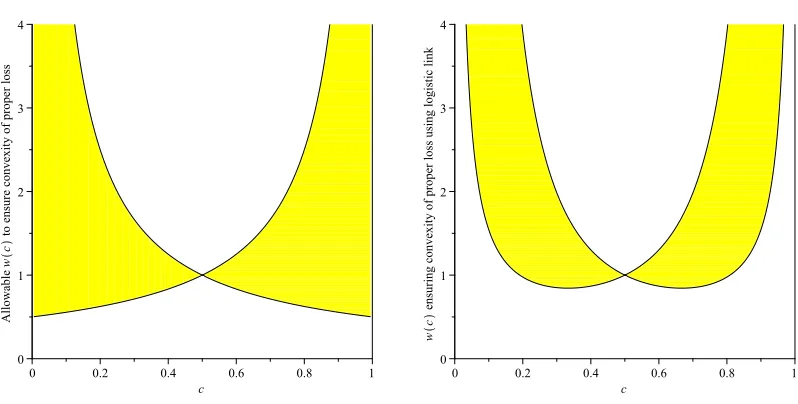
Figure 2: Allowable normalised weight functions to ensure convexity of composite loss functions with identity link (left) and logistic link (right).
Consider the linkψlogit(c):=log 1−cc
with corresponding inverse link q(c) = 1
1+e−c. One can
check thatψ′(c) = 1
c(1−c). Thus the constraints on the weight function w to ensure convexity of the
composite loss are
1
8x2(1−x) ⋚ w(x) ⋚ 1
8x(1−x)2, ∀x∈(0,1).
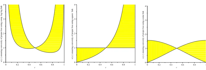
This is shown graphically in Figure 2. One can compute similar regions for any link. Two other examples are the Complementary Log-Log linkψCLL(x) =log(−log(1−x)) (confer McCullagh and Nelder, 1989), the “square link”ψsq(x) =x2and the “cosine link”ψcos(x) =1−cos(πx). All of these are illustrated in Figure 3. The reason for considering these last two rather unusual links is to illustrate the following fact. Observing that the allowable region in Figure 2 precludes weight functions that approach zero at the endpoints of the interval, and noting that in order to well approx-imate the behaviour of 0-1 loss (with its weight function being w0−1(c) =δ(c−12)) one would like a weight function that does indeed approach zero at the end points, it is natural to ask what constraints are imposed upon a linkψsuch that a composite loss with that link and a weight function w(c)such that
lim
cց0w(c) =climր1w(c) =0 (32)
Figure 3: Allowable normalised weight functions to ensure convexity of loss functions with com-plementary log-log, square and cosine links.
Corollary 30 If a loss is proper and convex, then it is strictly proper.
The proof of Corollary 30 makes use of the following special case of the Gronwall style Lemma 1.1.1 of Bainov and Simeonov (1992).
Lemma 31 Let b :R→Rbe continuous for t≥α. Let v(t)be differentiable for t≥αand suppose v′(t)≤b(t)v(t), for t≥αand v(α)≤v0. Then for t≥α,
v(t)≤v0exp
Z t
αb(s)ds
.
Proof (Corollary 30) Observe that the RHS of (17) implies
w′(v)≤ w(v)
1−v, v≥0.
Suppose w(0) =0. Then v0=0 and the settingα=0 the lemma implies w(t)≤v0exp
Z t
0 1 1−sds
= v0
1−t =0, t∈(0,1].
Thus if w(0) =0 then w(t) =0 for all t∈(0,1). Choosing any otherα∈(0,1)leads to a similar conclusion. Thus if w(t) =0 for some t∈[0,1), w(s) =0 for all s∈[t,1]. Hence w(t)>0 for all t∈[0,1]and hence by the remark immediately following Theorem 6ℓis strictly proper.
6.3 Convexity of Bregman Divergences in their Second Argument
7. Choosing a Surrogate Loss
A surrogate loss function is a loss function which is not exactly what one wishes to minimise but is easier to work with algorithmically. Convex surrogate losses are often used in place of the 0-1 loss which is not convex.
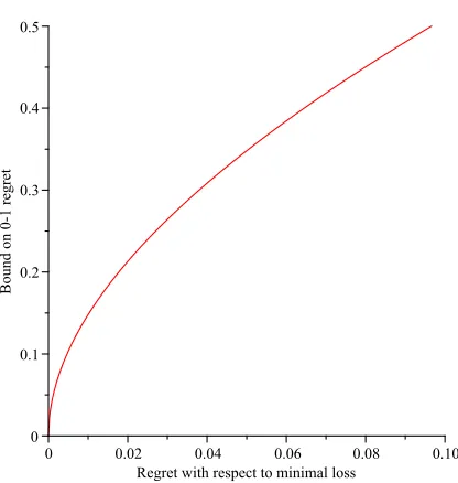
Surrogate losses have garnered increasing interest in the machine learning community (Zhang, 2004b; Bartlett et al., 2006; Steinwart, 2007; Steinwart and Christmann, 2008). Some of the ques-tions considered to date are bounding the regret of a desired loss in terms of a surrogate (“surrogate regret bounds”—see Reid and Williamson, 2009b and references therein), the relationship between the decision theoretic perspective and the elicitability perspective (Masnadi-Shirazi and Vascon-celos, 2009), and efficient algorithms for minimising convex surrogate margin losses (Nock and Nielsen, 2009b,a).
Typically convex surrogates are used because they lead to convex, and thus tractable, optimisa-tion problems. To date, work on surrogate losses has focussed on margin losses which necessarily are symmetric with respect to false positives and false negatives (Buja et al., 2005). In line with the rest of this paper, our treatment will not be so restricted.
The aim here is put forward some plausible definitions of what it might mean to select a “best” surrogate from a class of losses—for example, the class of proper, convex composite losses. We make use of the weight function perspective and the convexity results given in the previous section to investigate some new definitions for “best” surrogate and put forward some conjectures regarding them.
7.1 The “Best” Surrogate Loss
There are many choices of surrogate loss one can choose. A natural question is thus “which is best?”. In order to do this we need to first define how we are evaluating losses as surrogates. To do this we require notation to describe the set of minimisers of the conditional and full risk associated with a loss. Given a lossℓ:{−1,1} ×V→Rits conditional minimisers atη∈[0,1]is the set
H(ℓ,η):={v∈V: L(η,v) =L(η)}. (33)
Given a set of hypothesesH⊆VX, the (constrained) Bayes optimal risk is
LH:= inf
h∈HL(h,P).
The (full) minimisers overHforPis the set
H(ℓ,P):={h∈H:L(h) =LH},
whereH⊆VXis some restricted set of functions andL(h):=E(X,Y)∼P[ℓ(Y,h(X))]and the expec-tation is with respect toP. Given a reference lossℓref, we will say the ℓref-surrogate penalty of a lossℓover the function classHon a problem(η,M)(or equivalentlyP) is
Sℓref(ℓ,η,M) =Sℓref(ℓ,P):= inf
h∈H(ℓ,P)Lref(h),
where it is important to remember thatLis with respect toP. That is, Sℓref(ℓ,P)is the minimumℓref
Given a fixed experimentP, ifLis a class of losses then the best surrogate losses inLfor the reference lossℓref are those that minimise theℓref-surrogate penalty. This definition is motivated by the manner in which surrogate losses are used—one minimizesL(h)over h to obtain the minimiser h∗ and one hopes thatLref(h∗)is small. Clearly, if the class of losses contains the reference loss (i.e.,ℓref∈L) thenℓrefwill be a best surrogate loss. Therefore, the question of best surrogate loss is only interesting whenℓref∈/L. One particular case we will consider is when the reference loss is the 0-1 loss and the class of surrogatesLis the set of convex proper losses. Since 0-1 loss is not convex the question of which surrogate is best is non-trivial.
It would be nice if one could reason about the “best” surrogate loss using the conditional per-spective (that is working with L instead ofL) and in a manner independent of H. It is simple to see why this can not be done. Since all the losses we consider are proper, the minimiser over ˆηof L(η,ηˆ)isη. Thus any proper loss would lead to the same ˆη∈[0,1]. It is only the introduction of the restricted class of hypothesesHthat prevents this reasoning being applied forL: restrictions on h∈Hprevent h(x) =η(x)for all x∈X. We conclude that the problem of best surrogate loss only makes sense when one both takes expectations overXand restricts the class of hypotheses h to be drawn from some setH([0,1]X.
This reasoning accords with that of Nock and Nielsen (2009b,a) who examined which surrogate to use and proposed a data-dependent scheme that tunes surrogates for a problem. They explicitly considered proper losses and said that “minimizing any [lower-bounded, symmetric proper] loss amounts to the same ultimate goal” and concluded that “the crux of the choice of the [loss] relies on data-dependent considerations”.
We demonstrate the difficulty of finding a universal best surrogate loss in by constructing a simple example. One can construct experiments(η1,M)and(η2,M) and proper lossesℓ1 andℓ2 such that
Sℓ0−1(ℓ1,(η1,M))>Sℓ0−1(ℓ2,(η1,M)) but Sℓ0−1(ℓ1,(η2,M))<Sℓ0−1(ℓ2,(η2,M)).
(The examples we construct have weight functions that “cross-over” each other; the details are in Appendix A.) However, this does not imply there can not exist a particular convexℓ∗that minorizes
all proper losses in this sense. Indeed, we conjecture that, in the sense described above, there is no best proper, convex surrogate loss.
Conjecture 32 Given a proper, convex loss ℓthere exists a second proper, convex loss ℓ∗6=ℓ, a hypothesis classH, and an experimentPsuch that Sℓ0−1(ℓ
∗,P)<S
ℓ0−1(ℓ,P)for the classH.
To prove the above conjecture it would suffice to show that for a fixed hypothesis class and any pair of losses one can construct two experiments such that one loss minorises the other loss on one experiment and vice versa on the other experiment.
Supposing the above conjecture is true, one might then ask for a best surrogate loss for some reference lossℓref in a minimax sense. Formally, we would like the lossℓ∗∈Lsuch that the worst-case penalty for usingℓ∗,
ϒL(ℓ∗):=sup
P
Sℓref(ℓ
∗,P)−inf
ℓ∈LSℓref(ℓ,P)