Estimating High-Dimensional Directed Acyclic Graphs with the PC-Algorithm

Estimating High-Dimensional Directed Acyclic Graphs

with the PC-Algorithm

Markus Kalisch [email protected]

Peter B ¨uhlmann [email protected]

Seminar f¨ur Statistik ETH Zurich

8092 Z¨urich, Switzerland

Editor: David Maxwell Chickering

Abstract

We consider the PC-algorithm (Spirtes et al., 2000) for estimating the skeleton and equivalence class of a very high-dimensional directed acyclic graph (DAG) with corresponding Gaussian dis-tribution. The PC-algorithm is computationally feasible and often very fast for sparse problems with many nodes (variables), and it has the attractive property to automatically achieve high com-putational efficiency as a function of sparseness of the true underlying DAG. We prove uniform consistency of the algorithm for very high-dimensional, sparse DAGs where the number of nodes is allowed to quickly grow with sample size n, as fast as O(na)for any 0<a<∞. The sparseness assumption is rather minimal requiring only that the neighborhoods in the DAG are of lower order than sample size n. We also demonstrate the PC-algorithm for simulated data.

Keywords: asymptotic consistency, DAG, graphical model, PC-algorithm, skeleton

1. Introduction

Graphical models are a popular probabilistic tool to analyze and visualize conditional independence relationships between random variables (see Edwards, 2000; Lauritzen, 1996; Neapolitan, 2004). Major building blocks of the models are nodes, which represent random variables and edges, which encode conditional dependence relations of the enclosing vertices. The structure of conditional independence among the random variables can be explored using the Markov properties.

Of particular current interest are directed acyclic graphs (DAGs), containing directed rather than undirected edges, which restrict in a sense the conditional dependence relations. These graphs can be interpreted by applying the directed Markov property (see Lauritzen, 1996). When ignoring the directions of a DAG, we get the skeleton of a DAG. In general, it is different from the conditional independence graph (CIG), see Section 2.1. (Thus, estimation methods for directed graphs cannot be easily borrowed from approaches for undirected CIGs.) As we will see in Section 2.1, the skeleton can be interpreted easily and thus yields interesting insights into the dependence structure of the data.

1968; Heckerman et al., 1995), or a greedy search is employed. The greedy DAG search can be improved by exploiting probabilistic equivalence relations, and the search space can be reduced from individual DAGs to equivalence classes, as proposed in GES (Greedy Equivalent Search, see Chickering, 2002a). Although this method seems quite promising when having few or a moderate number of nodes, it is limited by the fact that the space of equivalence classes is conjectured to grow super-exponentially in the nodes as well (Gillispie and Perlman, 2001). Bayesian approaches for DAGs, which are computationally very intensive, include Spiegelhalter et al. (1993) and Heckerman et al. (1995).

An interesting alternative to greedy or structurally restricted approaches is the PC-algorithm (after its authors, Peter and Clark) from Spirtes et al. (2000). It starts from a complete, undirected graph and deletes recursively edges based on conditional independence decisions. This yields an undirected graph which can then be partially directed and further extended to represent the under-lying DAG (see later). The PC-algorithm runs in the worst case in exponential time (as a function of the number of nodes), but if the true underlying DAG is sparse, which is often a reasonable assumption, this reduces to a polynomial runtime.

In the past, interesting hybrid methods have been developed. Very recently, Tsamardinos et al. (2006) proposed a computationally very competitive algorithm. We also refer to their paper for a quite exhaustive numerical comparison study among a wide range of algorithms.

We focus in this paper on estimating the equivalence class and the skeleton of DAGs (corre-sponding to multivariate Gaussian distributions) in the high-dimensional context, that is, the number of nodes p may be much larger than sample size n. We prove that the PC-algorithm consistently es-timates the equivalence class and the skeleton of an underlying sparse DAG, as sample size n_→∞, even if p=pn=O(na) (0≤a<∞)is allowed to grow very quickly as a function of n.

Our implementation of the PC-algorithm is surprisingly fast, as illustrated in Section 4.5, and it allows us to estimate a sparse DAG even if p is in the thousands. For the high-dimensional setting with pn, sparsity of the underlying DAG is crucial for statistical consistency and computational

feasibility. Our analysis seems to be the first establishing a provable correct algorithm (in an asymp-totic sense) for high-dimensional DAGs which is computationally feasible.

The question of consistency of a class of methods including the PC algorithm has been treated in Spirtes et al. (2000) and Robins et al. (2003) in the context of causal inference. They show that, assuming only faithfulness (explained in Section 2), uniform consistency cannot be achieved, but pointwise consistency can. In this paper, we extend this in two ways: We provide a set of assumptions which renders the PC-algorithm to be uniformly consistent. More importantly, we show that consistency holds even as the number of nodes and neighbors increases and the size of the smallest non-zero partial correlations decrease as a function of the sample size. Stricter assumptions than the faithfulness condition that render uniform consistency possible have been also proposed in Zhang and Spirtes (2003). A rather general discussion on how many samples are needed to learn the correct structure of a Bayesian Network can be found in Zuk et al. (2006).

The problem of finding the equivalence class of a DAG has a substantial overlap with the prob-lem of feature selection: If the equivalence class is found, the Markov Blanket of any variable (node) can be read of easily. Given a set of nodes V and suppose that M is the Markov Blanket of node X , then X is conditionally independent of V_\M given M. Thus, M contains all and only the relevant

high dimensions or Ng (1998) for a rather general approach dealing with bounds for generalization errors.

2. Finding the Equivalence Class of a DAG

In this section, we first present the main concepts. Then, we give a detailed description of the PC-algorithm.

2.1 Definitions and Preliminaries

A graph G= (V,E)consists of a set of nodes or vertices V=_{1, . . . ,p_}and a set of edges E_⊆V_×V ,

that is, the edge set is a subset of ordered pairs of distinct nodes. In our setting, the set of nodes corresponds to the components of a random vector X_∈Rp. An edge(i,j)_∈E is called directed if (i,j)_∈E but(j,i)_∈/E; we then use the notation i_→ j. If both(i,j)_∈E and(j,i)_∈E, the edge

is called undirected; we then use the notation i₋j. A directed acyclic graph (DAG) is a graph G

where all edges are directed and not containing any cycle.

If there is a directed edge i_→ j, node i is said to be a parent of node j. The set of parents of

node j is denoted by pa(j). The adjacency set of a node j in graph G, denoted by ad j(G,j), are all nodes i which are directly connected to j by an edge (directed or undirected). The elements of

ad j(G,j)are also called neighbors of or adjacent to j.

A probability distribution P onRpis said to be faithful with respect to a graph G if conditional independencies of the distribution can be inferred from so-called d-separation in the graph G and vice-versa. More precisely: consider a random vector X∼P. Faithfulness of P with respect to G

means: for any i,j_∈V with i₆= j and any set s_⊆V ,

X(i)and X(j)are conditionally independent given_{X(r); r_∈s_}

⇔ node i and node j are d-separated by the set s.

The notion of d-separation can be defined via moral graphs; details are described in Lauritzen (1996, Prop. 3.25). We remark here that faithfulness is ruling out some classes of probability distributions. An example of a non-faithful distribution is given in Spirtes et al. (2000, Chapter 3.5.2). On the other hand, non-faithful distributions of the multivariate normal family (which we will limit ourselves to) form a Lebesgue null-set in the space of distributions associated with a DAG G, see Meek (1995a). The skeleton of a DAG G is the undirected graph obtained from G by substituting undirected edges for directed edges. A v-structure in a DAG G is an ordered triple of nodes(i,j,k)such that G contains the directed edges i_→ j and k_→ j, and i and k are not adjacent in G.

It is well known that for a probability distribution P which is generated from a DAG G, there is a whole equivalence class of DAGs with corresponding distribution P (see Chickering, 2002a, Section 2.2 ). Even when having infinitely many observations, we cannot distinguish among the different DAGs of an equivalence class. Using a result from Verma and Pearl (1990), we can characterize equivalent classes more precisely: Two DAGs are equivalent if and only if they have the same skeleton and the same v-structures.

A common tool for visualizing equivalence classes of DAGs are completed partially directed

acyclic graphs (CPDAG). A partially directed acyclic graph (PDAG) is a graph where some edges

and DAGs can be decided as for DAGs by inspecting the skeletons and v-structures. A PDAG is

completed, if (1) every directed edge exists also in every DAG belonging to the equivalence class

of the DAG and (2) for every undirected edge i₋j there exists a DAG with i_→ j and a DAG with i← j in the equivalence class.

CPDAGs encode all independence informations contained in the corresponding equivalence class. It was shown in Chickering (2002b) that two CPDAGs are identical if and only if they repre-sent the same equivalence class, that is, they reprerepre-sent a equivalence class uniquely.

Although the main goal is to identify the CPDAG, the skeleton itself already contains interesting information. In particular, if P is faithful with respect to a DAG G,

there is an edge between nodes i and j in the skeleton of DAG G

⇔ for all s_⊆V_{\ {}i,j_}, X(i)and X(j)are conditionally dependent

given_{X(r); r_∈s_}, (1)

(Spirtes et al., 2000, Th. 3.4). This implies that if P is faithful with respect to a DAG G, the skeleton of the DAG G is a subset (or equal) to the conditional independence graph (CIG) corresponding to P. (The reason is that an edge in a CIG requires only conditional dependence given the set

V_{\ {}i,j_}). More importantly, every edge in the skeleton indicates some strong dependence which cannot be explained away by accounting for other variables. We think, that this property is of value for exploratory analysis.

As we will see later in more detail, estimating the CPDAG consists of two main parts (which will naturally structure our analysis): (1) Estimation of the skeleton and (2) partial orientation of edges. All statistical inference is done in the first part, while the second is just application of deterministic rules on the results of the first part. Therefore, we will put much more emphasis on the analysis of the first part. If the first part is done correctly, the second will never fail. If, however, there occur errors in the first part, the second part will be more sensitive to it, since it depends on the inferential results of part (1) in greater detail. Therefore, when dealing with a high-dimensional setting (large

p, small n), the CPDAG is harder to recover than the skeleton. Moreover, the interpretation of

the CPDAG depends much more on the global correctness of the graph. The interpretation of the skeleton, on the other hand, depends only on a local region and is thus more reliable.

We conclude that, if the true underlying probability mechanisms are generated from a DAG, finding the CPDAG is the main goal. The skeleton itself oftentimes already provides interesting insights, and in a high-dimensional setting it might be interesting to use the undirected skeleton as an alternative target to the CPDAG when finding a useful approximation of the CPDAG seems hopeless.

As mentioned before, we will in the following describe two main steps. First, we will discuss the part of the PC-algorithm that leads to the skeleton. Afterwards we will complete the algorithm by discussing the extensions for finding the CPDAG. We will use the same format when discussing theoretical properties of the PC-algorithm.

2.2 The PC-algorithm for Finding the Skeleton

is used by the PC-algorithm which is able to exploit sparseness of the graph. More precisely, we apply the part of the PC-algorithm that identifies the undirected edges of the DAG.

2.2.1 POPULATIONVERSION FOR THESKELETON

In the population version of the PC-algorithm, we assume that perfect knowledge about all necessary conditional independence relations is available. We refer here to the PC-algorithm what others call the first part of the PC-algorithm; the other part is described in Algorithm 2 in Section 2.3.

Algorithm 1 The PCpop-algorithm

1: INPUT: Vertex Set V , Conditional Independence Information

2: OUTPUT: Estimated skeleton C, separation sets S (only needed when directing the skeleton afterwards)

3: Form the complete undirected graph ˜C on the vertex set V.

4: `=−1; C=C˜

5: repeat

6: `=`+1

7: repeat

8: Select a (new) ordered pair of nodes i, j that are adjacent in C such that_|ad j(C,i)_\{j_{}| ≥}`

9: repeat

10: Choose (new) k_⊆ad j(C,i)_{\ {}j_}with_|k_|=`.

11: if i and j are conditionally independent given k then

12: Delete edge i,j

13: Denote this new graph by C

14: Save k in S(i,j)and S(j,i)

15: end if

16: until edge i,j is deleted or all k⊆ad j(C,i)_{\ {}j}with|k|=`have been chosen

17: until all ordered pairs of adjacent variables i and j such that_|ad j(C,i)_{\ {}j_{}| ≥}`and k_⊆

ad j(C,i)_{\ {}j_}with_|k_|=`have been tested for conditional independence

18: until for each ordered pair of adjacent nodes i, j:|ad j(C,i)_{\ {}j}|< `.

The (first part of the) PC-algorithm is given in Algorithm 1. The maximal value of`in Algo-rithm 1 is denoted by

mreach= maximal reached value of`. (2)

The value of mreachdepends on the underlying distribution.

A proof that this algorithm produces the correct skeleton can be easily deduced from Theorem 5.1 in Spirtes et al. (2000). We summarize the result as follows.

Proposition 1 Consider a DAG G and assume that the distribution P is faithful to G. Denote the

maximal number of neighbors by q=max1≤j≤p|ad j(G,j)|. Then, the PCpop-algorithm constructs

the true skeleton of the DAG. Moreover, for the reached level: mreach∈ {q−1,q}.

2.2.2 SAMPLEVERSION FOR THESKELETON

For finite samples, we need to estimate conditional independencies. We limit ourselves to the Gaus-sian case, where all nodes correspond to random variables with a multivariate normal distribution. Furthermore, we assume faithful models, which means that the conditional independence relations correspond to d-separations (and so can be read off the graph) and vice versa; see Section 2.1.

In the Gaussian case, conditional independencies can be inferred from partial correlations.

Proposition 2 Assume that the distribution P of the random vector X is multivariate normal. For

i6= j∈ {1, . . . ,p}, k⊆ {1, . . . ,p} \ {i,j}, denote byρi,j|kthe partial correlation between X(i)and X(j)given_{X(r); r_∈k_}. Then,ρi,j_|k=0 if and only if X(i)and X(j)are conditionally independent given_{X(r); r_∈k_}.

Proof: The claim is an elementary property of the multivariate normal distribution, see Lauritzen

(1996, Prop. 5.2.).

We can thus estimate partial correlations to obtain estimates of conditional independencies. The sample partial correlation ˆρi,j|kcan be calculated via regression, inversion of parts of the covariance matrix or recursively by using the following identity: for some h_∈k,

ρi,j|k=

ρi,j_|k_\h−ρi,h_|k_\hρj,h_|k_\h

q (1−ρ2

i,h_|k_\h)(1−ρ2j,h_|k_\h) .

In the following, we will concentrate on the recursive approach. For testing whether a partial corre-lation is zero or not, we apply Fisher’s z-transform

Z(i,j_|k) =1

2log

₁₊ρ_ˆ

i,j_|k 1₋ρˆ_i,j|k

. (3)

Classical decision theory yields then the following rule when using the significance levelα. Reject the null-hypothesis H0(i,j_|k): ρi,j|k=0 against the two-sided alternative HA(i,j|k): ρi,j|k6=0 if

p

n_{− |}k_{| −}3_|Z(i,j_|k)_|>Φ−1₍₁₋α_{/2), where}Φ(_{·)denotes the cdf of}

N

The sample version of the PC-algorithm is almost identical to the population version in Section 2.2.1.

The PC-algorithm

Run the PCpop(m)-algorithm as described in Section 2.2.1 but replace in line 11 of Algorithm 1 the if-statement by

ifpn_{− |}k_{| −}3_|Z(i,j_|k)_{| ≤}Φ−1_{(1−α/2)then.}

The algorithm yields a data-dependent value ˆmreach,nwhich is the sample version of (2).

The only tuning parameter of the PC-algorithm isα, which is the significance level for testing partial correlations. See Section 4 for further discussion.

2.3 Extending the Skeleton to the Equivalence Class

While finding the skeleton as in Algorithm 1, we recorded the separation sets that made edges drop out in the variable denoted by S. This was not necessary for finding the skeleton itself, but will be essential for extending the skeleton to the equivalence class. In Algorithm 2 we describe the work of Pearl (2000, p.50f) to extend the skeleton to a CPDAG belonging to the equivalence class of the underlying DAG.

Algorithm 2 Extending the skeleton to a CPDAG INPUT: Skeleton Gskel, separation sets S OUTPUT: CPDAG G

for all pairs of nonadjacent variables i,j with common neighbour k do

if k_∈/S(i,j)then

Replace i₋k₋j in Gskelby i→k← j end if

end for

In the resulting PDAG, try to orient as many undirected edges as possible by repeated application of the following three rules:

R1 Orient j−k into j→k whenever there is an arrow i→ j such that i and k are nonadjacent.

R2 Orient i₋j into i_→ j whenever there is a chain i_→k_→ j.

R3 Orient i₋j into i_→ j whenever there are two chains i₋k_→ j and i₋l_→ j such that k and l are nonadjacent.

R4 Orient i₋j into i_→ j whenever there are two chains i₋k_→l and k_→l_→ j such that k and l are nonadjacent.

The output of Algorithm 2 is a CPDAG, which was first proved by Meek (1995b).

3. Consistency for High-Dimensional Data

As in Section 2, we will first deal with the problem of finding the skeleton. Consecutively, we will extend the result to finding the CPDAG.

3.1 Finding the Skeleton

We will show that the PC-algorithm from Section 2.2.2 is asymptotically consistent for the skeleton of a DAG, even if p is much larger than n but the DAG is sparse. We assume that the data are realizations of i.i.d. random vectors X1, . . . ,Xn with Xi∈Rp from a DAG G with corresponding distribution P. To capture high-dimensional behavior, we will let the dimension grow as a function of sample size: thus, p=pnand also the DAG G=Gnand the distribution P=Pn. Our assumptions are as follows.

(A1) The distribution Pnis multivariate Gaussian and faithful to the DAG Gnfor all n.

(A2) The dimension pn=O(na)for some 0_≤a<∞.

(A3) The maximal number of neighbors in the DAG Gnis denoted by

qn=max1≤j≤pn|ad j(G,j)|, with qn=O(n

(A4) The partial correlations between X(i)and X(j)given{X(r); r∈k}for some set k⊆ {1, . . . ,pn}\

{i,j_}are denoted byρn;i,j|k. Their absolute values are bounded from below and above:

inf_{|ρi,j_|k|; i,j,k withρi,j_|k6=0} ≥cn, cn−1=O(nd), for some 0<d<b/2,

sup n;i,j,k|

ρi,j|k| ≤M<1,

where 0<b≤1 is as in (A3).

Assumption (A1) is an often used assumption in graphical modeling, although it does restrict the class of possible probability distributions (see also third paragraph of Section 2.1); (A2) al-lows for an arbitrary polynomial growth of dimension as a function of sample size, that is, high-dimensionality; (A3) is a sparseness assumption and (A4) is a regularity condition. Assumptions (A3) and (A4) are rather minimal: note that with b=1 in (A3), for example fixed qn=q<∞, the partial correlations can decay as n−1/2+εfor any 0<ε_≤1/2. If the dimension p is fixed (with fixed DAG G and fixed distribution P), (A2) and (A3) hold and (A1) and the second part of (A4) remain as the only conditions. Recently, for undirected graphs the Lasso has been proposed as a computa-tionally efficient algorithm for estimating high-dimensional conditional independence graphs where the growth in dimensionality is as in (A2) (see Meinshausen and B ¨uhlmann, 2006). However, the Lasso approach can be inconsistent, even with fixed dimension p, as discussed in detail in Zhao and Yu (2006).

Theorem 1 Assume (A1)-(A4). Denote by ˆGskel,n(αn)the estimate from the (first part of the)

PC-algorithm in Section 2.2.2 and by Gskel,n the true skeleton from the DAG Gn. Then, there exists

αn→0(n→∞), see below, such that

IP[Gˆskel,n(αn) =Gskel,n]

= 1₋O(exp(₋Cn1−2d))_→1(n_→∞)for some 0<C<∞, where d>0 is as in (A4).

A proof is given in the Section A. A choice for the value of the significance level is αn= 2(1−Φ(n1/2cn/2))which depends on the unknown lower bound of partial correlations in (A4). 3.2 Extending the Skeleton to the Equivalence Class

As mentioned before, all inference is done while finding the skeleton. If this part is completed perfectly, that is, if there was no error while testing conditional independencies (it is not enough to assume that the skeleton was estimated correctly), the second part will never fail (see Meek, 1995b). Therefore, we easily obtain:

Theorem 2 Assume (A1)-(A4). Denote by ˆGCPDAG(αn)the estimate from the entire PC-algorithm

in Section 2.2.2 and 2.3 and by GCPDAG the true CPDAG from the DAG G. Then, there exists

αn→0(n→∞), see below, such that

IP[_Gˆ_{CPDAG(αn) =GCPDAG]}

A proof, consisting of one short argument, is given in the Section A. As for Theorem 1, we can chooseαn=2(1−Φ(n1/2cn/2)).

By inspecting the proofs of Theorem 1 and Theorem 2, one can derive explicit error bounds for the error probabilities. Roughly speaking, this bounding function is the product of a linearly increasing and an exponentially decreasing term (in n). The bound is loose but for completeness, we present it in the Appendix.

4. Numerical Examples

We analyze the PC-algorithm for finding the skeleton and the CPDAG using various simulated data sets. The numerical results have been obtained using theR-packagepcalg. For an extensive numerical comparison study of different algorithms, we refer to Tsamardinos et al. (2006).

4.1 Simulating Data

In this section, we analyze the PC-algorithm for the skeleton using simulated data. In order to simulate data, we first construct an adjacency matrix A as follows:

1. Fix an ordering of the variables.

2. Fill the adjacency matrix A with zeros.

3. Replace every matrix entry in the lower triangle (below the diagonal) by independent realiza-tions of Bernoulli(s) random variables with success probability s where 0<s<1. We will call s the sparseness of the model.

4. Replace each entry with a 1 in the adjacency matrix by independent realizations of a Uniform([0.1,1]) random variable.

This then yields a matrix A whose entries are zero or in the range[0.1,1]. The corresponding DAG draws a directed edge from node i to node j if i< j and Aji6=0. The DAGs (and skeletons thereof) that are created in this way have the following property: IE[Ni] =s(p−1), where Ni is the number of neighbors of a node i.

Thus, a low sparseness parameter s implies few neighbors and vice-versa. The matrix A will be used to generate the data as follows. The value of the random variable X(1), corresponding to the first node, is given by

ε(1)_∼N(0,1), X(1)=ε(1),

and the values of the next random variables (corresponding to the next nodes) can be computed recursively as

ε(i)_∼N(0,1),

X(i)=

i−1

∑

k=1

AikX(k)+ε(i)(i=2, . . . ,p),

4.2 Choice of Significance Level

In Section 3 we provided a value of the significance levelαn=2(1−Φ(n1/2cn/2)). Unfortunately, this value is not constructive, since it depends on the unknown lower bound of partial correlations in (A4). To get a feeling for good values of the significance level in the domain of realistic parameter settings, we fitted a wide range of parameter settings and compared the quality of fit for different significance levels.

Assessing the quality of fit is not quite straightforward, since one has to examine simultaneously both the true positive rate (TPR) and false positive rate (FPR) for a meaningful comparison. We fol-low an approach suggested by Tsamardinos et al. (2006) and use the Structural Hamming Distance (SHD). Roughly speaking, this counts the number of edge insertions, deletions and flips in order to transfer the estimated CPDAG into the correct CPDAG. Thus, a large SHD indicates a poor fit, while a small SHD indicates a good fit.

We fitted 40 replicates to all combinations of

• α∈ {0.00005,0.0001,0.0005,0.001,0.005,0.01,0.05,0.1_},

• p_{∈ {}7,15,40,70,100_},

• n_{∈ {}30,100,300,1000,3000,10000,30000_},

• E[N]_{∈ {}2,5_},

(where E[N]is the average neighborhood size) and evaluated the SHD. Each value ofαwas used 40 times on each of the 70 possible parameter settings, and we then computed the average SHD over the 70 parameter settings.

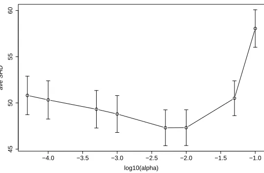
The result is shown in Figure 1. One can see that the average SHD achieves a minimum in the region aroundα=0.005 andα=0.01. For higher or lower significance levels, the average SHD increases; the increase for bigger significance levels is much more pronounced. We analyzed the results of the simulation (see Figure 1) using pairwise Wilcoxon-Tests and Bonferroni correction. It turns out thatα=0.005 andα=0.01 yield significantly lower average SHD than the other values of α. In contrast, there is no significant difference between α=0.005 and α=0.001 (without Bonferroni correction). Of course, if n was of different order of magnitude, a reasonableαshould be a function of n withα=αn→0(n→∞).

4.3 Performance for Different Parameter Settings

In this section, we give an overview over the performance in terms of the true positive rate (TPR) and false positive rate (FPR) for the skeleton and the SHD for the CPDAG. In order to keep the overview at a manageable size, we restrict the significance level to α=0.01. This was one of the two settings minimizing the average SHD as described in the previous section. The remaining parameters will be chosen as follows:

• p_{∈ {}7,40,100_},

• n_{∈ {}30,100,300,1000,3000,10000,30000_},

−4.0 −3.5 −3.0 −2.5 −2.0 −1.5 −1.0

45

50

55

60

log10(alpha)

ave SHD

Figure 1: Average Structural Hamming Distance (ave SHD) with 95% confidence intervals. For each value of α, the average SHD was averaged over 70 parameter settings using 40 replicates each. One can see that the average SHD is minimized for significance levels betweenα=0.005 andα=0.01.

The overview is given in Figure 2. As expected, the fit for a dense graph (triangles; E[N] =5) is worse than the fit for a sparse graph (circles; E[N] =2). While the TPR and the SHD show a clear tendency with increasing sample size, the behavior of FPR is not so clear. The latter seems surprising at first sight but is due to the fact that we used the sameα=0.01 for all n.

4.4 Properties in High-Dimensional Setting

In this section, we study the behaviour of the error rates in a high-dimensional setting. The number of variables increases exponentially, the number of samples increases linearly and the expected neighborhood size increases sub-linearly. By inspecting the theory, we would expect the error rates to stay constant or even decrease. Table 1 shows the parameter setting of a small numerical study addressing this question. Note that p increases exponentially, n increases linearly and the expected neighborhood size E[N] =0.2√n increases sub-linearly. We usedα=0.05 and the results are based on 20 simulation runs.

Figure 3 shows boxplots of the TPR and the FPR over 20 replicates of this study. One can easily see that the TPR increases and the FPR decreases with sample size, although the number of p=pn grows fast and E[N]grows slowly with n. This confirms our theory very clearly.

1.5 2.0 2.5 3.0 3.5 4.0 4.5 0.2 0.6 1.0 log10(n) TPR (p=7) TPR

1.5 2.0 2.5 3.0 3.5 4.0 4.5

0.00 0.15 0.30 log10(n) FPR FPR

1.5 2.0 2.5 3.0 3.5 4.0 4.5

5 10 15 log10(n) SHD SHD

1.5 2.0 2.5 3.0 3.5 4.0 4.5

0.2

0.6

1.0

log10(n)

TPR (p=40)

1.5 2.0 2.5 3.0 3.5 4.0 4.5

0.002

0.008

log10(n)

FPR

1.5 2.0 2.5 3.0 3.5 4.0 4.5

20

60

100

log10(n)

SHD

1.5 2.0 2.5 3.0 3.5 4.0 4.5

0.2

0.6

1.0

log10(n)

TPR (p=100)

1.5 2.0 2.5 3.0 3.5 4.0 4.5

0.0010

0.0020

log10(n)

FPR

1.5 2.0 2.5 3.0 3.5 4.0 4.5

50

150

250

log10(n)

SHD

Figure 2: Performance of the PC-algorithm for different parameter settings, showing the mean of TPR, FPR and SHD together with 95% confidence intervals. The triangles represent parameter settings where E[N] =5, while the circles represent parameter settings where

E[N] =2.

p n E[N] TPR FPR

9 50 1.4 0.61 (0.03) 0.023 (0.005) 27 100 2.0 0.70 (0.02) 0.011 (0.001) 81 150 2.4 0.753 (0.007) 0.0065 (0.0003) 243 200 2.8 0.774 (0.004) 0.0040 (0.0001) 729 250 3.2 0.794 (0.004) 0.0022 (0.00004) 2187 300 3.5 0.805 (0.002) 0.0012 (0.00002)

Table 1: The number of variables p increases exponentially, the sample size n increases linearly and the expected neighborhood size E[N]increases sub-linearly. As supported by theory, the TPR increases and the FPR decreases in this setting. The results are based on using

p=9 p=27 p=81 p=243 p=729 p=2187

0.4

0.5

0.6

0.7

0.8

0.9

TPR

p=9 p=27 p=81 p=243 p=729 p=2187

0.00

0.02

0.04

0.06

FPR

Figure 3: While the number of variables p increases exponentially, the sample size n increases lin-early and the expected neighborhood size E[N]increases sub-linearly, the TPR increases and the FPR decreases. See Table 1 for a more detailed specification of the parameters.

4.5 Computational Complexity

Our theoretical framework in Section 3 allows for large values of p. The computational complexity of the PC-algorithm is difficult to evaluate exactly, but the worst case is bounded by

O(pmˆreach_{)which is with high probability bounded by O(p}q_{) (4)}

as a function of dimensionality p; here, q is the maximal size of the neighborhoods as described in assumption (A3) in Section 3. We note that the bound may be very loose for many distributions. Thus, for the worst case where the complexity bound is achieved, the algorithm is computationally feasible if q is small, say q_≤3, even if p is large. For non-worst cases, however, we can still do the computations for much larger values of q and fairly dense graphs, for example some nodes j having neighborhoods of size up to_|ad j(G,j)_|=30.

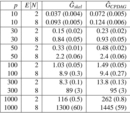
We provide a small example of the processor time for estimating a CPDAG by using the PC-algorithm. The runtime analysis was done on an AMD Athlon 64 X2 Dual Core Processor 5000+ with 2.6 GHz and 4 GB RAM running on Linux and using R 2.4.1. The number of variables varied between p=10 and p=1000 while the number of samples was fixed at n=1000. The sparseness was either E[N] =2 or E[N] =8. For each parameter setting, 10 replicates were used. In each case, the significance level used in the PC-algorithm wasα=0.01. The average processor time together with its standard deviation for estimating both the skeleton and the CPDAG is given in Table 2. Graphs of p=1000 nodes and 8 neighbors on average could be estimated in about 25 minutes, while networks with up to p=100 nodes could be estimated in about a second. The additional time spent for finding the CPDAG from the skeleton is comparable for both neighborhood sizes and varies between a couple to almost 100 percent of the time needed to estimate the skeleton. The percentage tends to decrease with increasing number of variables.

plot; therefore, the slope of the lines indicates the exponent of polynomial growth. In this case, both curves follow very roughly a line with slope two indicating quadratic growth. The positive curvature of the solid line would indicate exponential growth; theory tells us, that this is not possible. One possible explanation for the positive curvature is the fact, that with increasing p, the maximal neighborhood size (which was not controlled in the simulation) is likely to increase. This would gradually increase the exponent in the polynomial growth of the upper bound in Formula (4), thus yielding a positive curvature.

p E[N] _Gˆ_{skel G}ˆ_CPDAG 10 2 0.037 (0.004) 0.072 (0.005) 10 8 0.093 (0.005) 0.124 (0.006) 30 2 0.15 (0.02) 0.23 (0.02) 30 8 0.84 (0.05) 0.93 (0.05) 50 2 0.33 (0.01) 0.48 (0.02) 50 8 2.2 (0.06) 2.4 (0.06) 100 2 1.03 (0.05) 1.49 (0.05) 100 8 8.9 (0.3) 9.4 (0.27) 300 2 8.3 (0.1) 13.8 (0.13)

300 8 89 (3) 95 (3)

1000 2 116 (0.5) 262 (0.8) 1000 8 1300 (60) 1445 (59)

Table 2: The average processor time (Athl. 64, 2.6 GHz, 4 GB) for estimating the skeleton ( ˆGskel) or the CPDAG ( ˆGCPDAG) for different DAGs in seconds, with standard errors in brackets. We usedα=0.01 and sample size n=1000.

5. R-Packagepcalg

The R-packagepcalgcan be used to estimate from data the underlying skeleton or equivalence class of a DAG. To use this package, the statistics softwareRneeds to be installed. BothR and the R-packagepcalgare available free of charge athttp://www.r-project.org. For low-dimensional problems (but not for p in the hundreds or thousands), there are a number of other implementations of the PC-algorithm that are also worth mentioning:

• Hugin athttp://www.hugin.com.

• Murphy’s Bayes Network toolbox athttp://bnt.sourceforge.net.

• Tetrad IV athttp://www.phil.cmu.edu/projects/tetrad.

1.0 1.5 2.0 2.5 3.0

−1

0

1

2

3

log10(p)

log10( Processor Time [s] )

E[N]=2 E[N]=8

Figure 4: Average processor time over 10 runs together with 95% confidence intervals. Triangles correspond to dense (E[N] =8), circles to sparse (E[N] =2) underlying DAGs. We used

α=0.01 and sample size n=1000.

library(pcalg) ## define parameters

p <- 10 # number of random variables n <- 10000 # number of samples s <- 0.4 # sparsness of the graph For simulating data as described in Section 4.1:

## generate random data set.seed(42)

g <- randomDAG(p,s) # generate a random DAG d <- rmvDAG(n,g) # generate random samples

Then we estimate the underlying skeleton by using the functionpcAlgoand extend the skeleton to the CPDAG by using the functionudag2cpdag.

gSkel

<-pcAlgo(d,alpha=0.05) # estimate of the skeleton gCPDAG

<-udag2cpdag(gSkel)

The CPDAG can also be estimated directly using

gCPDAG

1

2

3

4 5

6

7 8

9

10

(a) True DAG

pcAlgo(dm = d, alpha = 0.05)

1

2

3

4

5

6

7

8

9

10

(b) Estimated Skeleton

pcAlgo(dm = d, alpha = 0.05)

1

2

3

4

5

6

7

8

9

10

(c) Estimated CPDAG

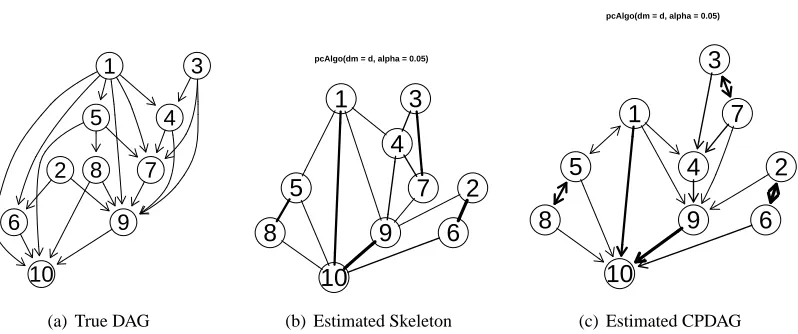
Figure 5: Plots generated using theR-packagepcalgas described in Section 5. (a) The true DAG. (b) The estimated skeleton using theR-functionpcAlgowithα=0.05 and n=10000. Line width encodes the reliability (z-values) of the dependence estimates (thick lines are reliable). (c) The estimated CPDAG using theR-functionudag2cpdag. Double-headed arrows indicate undirected edges.

plot(g)

plot(gSkel,zvalue.lwd=TRUE) plot(gCPDAG,zvalue.lwd=TRUE)

The original DAG is shown in Figure 5(a). The estimated skeleton and the estimated CPDAG are shown in Figure 5(b) and Figure 5(c), respectively. Note the differing line width, which indicates the reliability (z-values as in Formula 3) of the involved statistical tests (thick lines are reliable).

6. Conclusions

We show that the PC-algorithm is asymptotically consistent for the equivalence class of the DAG (represented by the CPDAG) and its skeleton with corresponding very high-dimensional, sparse Gaussian distribution. Moreover, the PC-algorithm is computationally feasible for such high-dimen-sional, sparse problems. Putting these two facts together, the PC-algorithm is established as a method (so far the only one) which is computationally feasible and provably correct, in the sense of uniform consistency, for high-dimensional DAGs. Sparsity, in terms of the maximal size of the neighborhoods of the true underlying DAG, is crucial for statistical consistency (assumption (A3) and Theorems 1 and 2) and for computational feasibility with at most a polynomial complexity (see Formula 4) as a function of dimensionality.

Acknowledgments

We would like to thank Martin M¨achler for his help with developing the R-packagepcalg. We also thank three anonymous reviewers and the editor for their constructive comments. Markus Kalisch was supported by the Swiss National Science Foundation (grant no. 200021-105276 and 200020-113270/1).

Appendix A. Proofs

In the following, we give the proofs of all our theorems.

A.1 Proof of Proposition 1

Consider X with distribution P. Since P is faithful to the DAG G, conditional independence of X(i) and X(j) given_{X(r); r_∈k_}(k_⊆V_{\ {}i,j_}) is equivalent to d-separation of nodes i and j given the set k (see Spirtes et al., 2000, Th. 3.3). Thus, the population PCpop-algorithm as formulated in Section 2.2.1 coincides with the one from Spirtes et al. (2000) which is using the concept of d-separation, and the first claim about correctness of the skeleton follows from Spirtes et al. (2000, Th. 5.1., Ch. 13).

The second claim about the value of mreachcan be proved as follows. First, due to the definition of the PCpop-algorithm and the fact that it constructs the correct skeleton, mreach_≤q. We now

argue that mreach≥q−1. Suppose the contrary. Then, mreach≤q−2: we could then continue with a further iteration in the algorithm since mreach+1≤q−1 and there is at least one node j with neighborhood-size_|ad j(G,j)_|=q: that is, the reached stopping level would be at least q₋1 which

is a contradiction to mreach≤q−2.

A.2 Analysis of the PC-Algorithm

When analyzing the consistency of the PC-algorithm, the convergence properties of partial correla-tions turn out to be crucial. Therefore, we first concentrate on partial correlacorrela-tions and then shift our focus to the analysis of the PC-algorithm.

A.2.1 ANALYSIS OFPARTIALCORRELATIONS

We first establish uniform consistency of estimated partial correlations. Denote by ˆρi,j and ρi,j the sample and population correlation between X(i) and X(j). Likewise, ˆρi,j|k and ρi,j|k denote the sample and population partial correlation between X(i) and X(j) given _{X(r); r_∈k_}, where k_{⊆ {}1, . . . ,pn} \ {i,j}.

Many partial correlations (and non-partial correlations) are tested for being zero during the run of the PC(mn)-algorithm. For a fixed ordered pair of nodes i,j, the conditioning sets are elements of

Kmn

i,j ={k⊆ {1, . . . ,pn} \ {i,j}:|k| ≤mn}

whose cardinality is bounded by

|Kmn

Lemma 1 Assume (A1) (without requiring faithfulness) and sup_n,i6=j|ρn;i,j| ≤M<1 (compare with

(A4)). Then, for any 0<γ_≤2,

sup i,j,k∈Kimn,j

IP[_|ρˆn;i,j−ρn;i,j|>γ]≤C1(n−2)exp

(n₋4)log(4−γ

2 4+γ2)

,

for some constant 0<C1<∞depending on M only.

Proof: We make substantial use of Hotelling (1953)’s work. Denote by fn(ρˆ,ρ) the probability density function of the sample correlation ˆρ=ρˆn+1;i,jbased on n+1 observations and byρ=ρn+1;i,j the population correlation. (It is notationally easier to work with sample size n+1; and we just use the abbreviated notations with ˆρandρ). For 0<γ_≤2,

IP[_|ρˆ₋ρ_|>γ] =IP[ρˆ <ρ₋γ] +IP[ρˆ >ρ+γ].

It can be shown, that fn(r,ρ) = fn(−r,−ρ), see Hotelling (1953, p.201). This symmetry implies,

IPρ[ρˆ <ρ₋γ] =IP˜ρ[ρˆ >ρ˜+γ]with ˜ρ=₋ρ. (6)

Thus, it suffices to show that IP[ρˆ >ρ+γ] =IP_ρ[ρˆ >ρ+γ]decays exponentially in n, uniformly for allρ.

It has been shown (Hotelling, 1953, p.201, Formula (29)), that for₋1<ρ<1,

IP[ρˆ >ρ+γ]_≤√(n−1)Γ(n)

2πΓ(n+1₂)M0(ρ+γ)(1+

2

1_{− |}ρ_|) (7)

with

M0(ρ+γ) = Z 1

ρ+γ(1−ρ

2₎n_2(1−x2₎n−3_{2 (1−ρx)}−n+1 2dx

=

Z 1

ρ+γ(1−ρ

2₎n˜+₂3₍₁

−x2)n2˜(₁−ρ_x)−n˜−

5

2_dx (_{using ˜n}=_n−₃)

≤ (1−ρ

2₎3₂

(1_{− |}ρ_|)52

Z 1

ρ+γ( p

1₋ρ2√_1−x2 1₋ρx )

˜ n_dx

≤ (1−ρ

2₎3₂

(1_{− |}ρ_|)52

2 max

ρ+γ≤x≤1(

p

1₋ρ2√_1−x2 1₋ρx )

˜

n_{. (8)}

We will show now that g_ρ(x) = √

1−ρ2√_1−x2

1−ρx <1 for all ρ+γ≤x≤1 and −1<ρ<1 (in fact,

ρ_≤1₋γdue to the first restriction). Consider

sup −1<ρ<1;ρ+γ≤x≤1

gρ(x) = sup −1<ρ≤1−γ

p

1₋ρ2p

1₋(ρ+γ)2 1₋ρ(ρ+γ)

= q

1₋γ₄2

q

1₋γ₄2 1₋(−₂γ)(₂γ) =

4₋γ2

Therefore, for−1<₋M≤ρ≤M<1 (see assumption (A4)) and using Formulas (7)-(9) to-gether with the fact that _Γ(Γ(_nn)

+1 2)≤

const.with respect to n, we have

IP[ρˆ>ρ+γ]

≤ √(n−1)Γ(n)

2πΓ(n+1 2)

(1₋ρ2)32

(1_{− |}ρ_|)52

2(4−γ

2 4+γ2)

˜

n₍₁₊ 2 1_{− |}ρ_|)

≤ √(n−1)Γ(n)

2πΓ(n+1 2)

1

(1₋M)52

2(4−γ

2 4+γ2)

˜

n₍₁₊ 2 1₋M)≤

≤ C1(n−1)(

4₋γ2 4+γ2)

˜ n_=C

1(n−1)exp((n−3)log( 4₋γ2 4+γ2)),

where 0<C1<∞depends on M only, but not onρ orγ. By invoking Formula (6), the proof is complete (note that the proof assumed sample size n+1).

Lemma 1 can be easily extended to partial correlations, as shown by Fisher (1924), using pro-jections for Gaussian distributions.

Lemma 2 (Fisher, 1924)

Assume (A1) (without requiring faithfulness). If the cumulative distribution function of ˆρn;i,j is

denoted by F(_·|n,ρn;i,j), then the cdf of the sample partial correlation ˆρn;i,j|kwith|k|=m<n−1 is F[_·|n₋m,ρ_n;i,j|k]. That is, the effective sample size is reduced by m.

A proof can be found in Fisher (1924); see also Anderson (1984).

Lemma 1 and 2 yield then the following.

Corollary 1 Assume (the first part of) (A1) and (the upper bound in) (A4). Then, for anyγ>0,

sup i,j,k∈Kimn,j

IP[_|ρˆ_n;i,j|k−ρ_n;i,j|k|>γ]

≤ C1(n−2−mn)exp

(n₋4₋mn)log( 4₋γ2 4+γ2)

,

for some constant 0<C1<∞depending on M from (A4) only.

The PC-algorithm is testing partial correlations after the z-transform g(ρ) =0.5 log((1+ρ)/(1₋

ρ)). Denote by Z_n;i,j|k=g(ρˆ_n;i,j|k)and by z_n;i,j|k=g(ρ_n;i,j|k).

Lemma 3 Assume the conditions from Corollary 1. Then, for anyγ>0,

sup i,j,k∈K_imn_,j

IP[_|Zn;i,j_|k−zn;i,j_|k|>γ]

≤ O(n₋mn)

exp((n₋4₋mn)log(

4₋(γ/L)2

4+ (γ/L)2)) +exp(−C2(n−mn))

Proof: A Taylor expansion of the z-transform g(ρ) =0.5 log((1+ρ)/(1−ρ))yields:

Zn;i,j|k−zn;i,j|k=g0(ρ˜n;i,j|k)(ρˆn;i,j|k−ρn;i,j|k), (10)

where_|ρ˜_n;i,j|k−ρ_{n;i,j|k| ≤ |}ρˆ_n;i,j|k−ρ_n;i,j|k|. Moreover, g0(ρ) =1/(1₋ρ2). By applying Corollary 1 withγ=κ= (1₋M)/2 we have

sup i,j,k∈K_imn_,j

IP[_|ρ˜_n;i,j|k−ρ_{n;i,j|k| ≤}κ]

> 1₋C1(n−2−mn)exp(−C2(n−mn)). (11) Since

g0(ρ˜_n;i,j|k) = 1

1₋ρ˜2 n;i,j|k

= 1

1₋(ρn;i,j|k+ (ρ˜n;i,j|k−ρn;i,j|k))2

≤ ₁ 1

−(M+κ)2 if|ρ˜n;i,j|k−ρn;i,j|k| ≤κ,

where we also invoke (the second part of) assumption (A4) for the last inequality. Therefore, since

κ= (1₋M)/2 yielding 1/(1₋(M+κ)2_{) =L, and using Formula (11), we get} sup

i,j,k∈Kimn,j

IP[_|g0(ρ˜_n;i,j|k)_{| ≤}L]

≥ 1₋C1(n−2−mn)exp(−C2(n−mn)). (12)

Since_|g0(ρ)_{| ≥}1 for allρ, we obtain with Formula (10):

sup i,j,k∈K_imn_,j

IP[_|Z_n;i,j|k−z_n;i,j|k|>γ] (13)

≤ sup

i,j,k_∈K_imn_,j

IP[_|g0(ρ˜_n;i,j|k)_|>L] + sup i,j,k_∈K_imn_,j

IP[_|ρˆ_n;i,j|k−ρ_n;i,j|k|>γ/L].

Formula (13) follows from elementary probability calculations: for two random variables U,V

with_|U_{| ≥}1 (_|U_|corresponding to_|g0(ρ)˜ _|and_|V_|to the difference_|ρˆ₋ρ_|),

IP[_|UV_|>γ] = IP[_|UV_|>γ,_|U_|>L] +IP[_|UV_|>γ,1_{≤ |}U_{| ≤}L]

≤ IP[_|U_|>L] +IP[_|V_|>γ/L].

The statement then follows from Formulas (13), (12) and Corollary 1.

A.2.2 PROOF OFTHEOREM1

For the analysis of the PC-algorithm, it is useful to consider a more general version as shown in Algorithm 3.

The PC-algorithm in Section 2.2.1 equals the PCpop(mreach)-algorithm . There is the obvious sample version, the PC(m)-algorithm, and the PC-algorithm in Section 2.2.2 is then same as the PC( ˆmreach)-algorithm, where ˆmreachis the sample version of Formula (2).

Algorithm 3 The PCpop(m)-algorithm

INPUT: Stopping level m, Vertex Set V , Conditional Independence Information

OUTPUT: Estimated skeleton C, separation sets S (only needed when directing the skeleton afterwards)

Form the complete undirected graph ˜C on the vertex set V. `=₋1; C=_C˜

repeat `=`+1 repeat

Select a (new) ordered pair of nodes i, j that are adjacent in C such that_|ad j(C,i)_{\ {}j_{}| ≥}` repeat

Choose (new) k_⊆ad j(C,i)_{\ {}j_}with_|k_|=`. if i and j are conditionally independent given k then

Delete edge i,j

Denote this new graph by C. Save k in S(i,j)and S(j,i)

end if

until edge i,j is deleted or all k_⊆ad j(C,i)_{\ {}j_}with_|k_|=`have been chosen

until all ordered pairs of adjacent variables i and j such that_|ad j(C,i)_{\ {}j_{}| ≥}`and k_⊆

ad j(C,i)_{\ {}j_}with_|k_|=`have been tested for conditional independence until`=m or for each ordered pair of adjacent nodes i, j:_|ad j(C,i)_{\ {}j_}|< `.

Lemma 4 Assume (A1), (A2), (A3) where 0<b_≤1 and (A4) where 0<d <b/2. Denote by ˆ

Gskel,n(αn,mn) the estimate from the PC(mn)-algorithm in Section 2.2.2 and by Gskel,n the true

skeleton from the DAG Gn. Moreover, denote by mreach,n the value described in (2). Then, for

mn≥mreach,n, mn=O(n1−b) (n→∞), there existsαn→0(n→∞)such that IP[Gˆskel,n(αn,mn) =Gskel,n]

= 1₋O(exp(₋Cn1−2d))_→1(n_→∞)for some 0<C<∞.

Proof: An error occurs in the sample PC-algorithm if there is a pair of nodes i,j and a

con-ditioning set k_∈Kmn

i,j (although the algorithm is typically only going through a random subset of

Kmn

i,j) where an error event Ei,j_|koccurs; Ei,j,kdenotes that “an error occurred when testing partial correlation for zero at nodes i,j with conditioning set k”. Thus,

IP[an error occurs in the PC(mn)-algorithm]

≤ P[ [

i,j,k∈Ki jmn

Ei,j|k]≤O(pmnn+2) sup i,j,k∈Ki jmn

IP[Ei,j|k], (14)

using that the cardinality of the set_|{i,j,k_∈Kmn

i j }|=O(pmnn+2), see also Formula 5. Now

Ei,j|k=EiI,j|k∪EiII,j|k, (15)

where

type I error E_iI_,j|k: pn_{− |}k_{| −}3_|Z_i,j|k|>Φ−1_{(1−α/2)and z}

Chooseα=αn=2(1−Φ(n1/2cn/2)), where cnis from (A4). Then, sup

i,j,k∈K_imn_,j

IP[E_iI_,j|k] = sup i,j,k∈K_imn_,j

IP[_|Zi,j_|k−zi,j_|k|>(n/(n− |k| −3))1/2cn/2]

≤ O(n₋mn)exp(−C3(n−mn)c2n), (16)

for some 0<C3<∞using Lemma 3 and the fact that log(4−δ

2

4+δ2)∼ −δ2/2 asδ→0. Furthermore,

with the choice ofα=αnabove,

sup i,j,k∈Kimn,j

IP[E_iII_,j|k] = sup i,j,k∈Kimn,j

IP[_|Zi,j|k| ≤

p

n/(n_{− |}k_{| −}3)cn/2]

≤ sup

i,j,k∈Kimn,j

IP[_|Zi,j|k−zi,j|k|>cn(1−

p

n/(n_{− |}k_{| −}3)/2)],

because inf_i,j;k∈Kmn

i,j |zi,j|k| ≥cnsince|g(ρ)| ≥ |ρ|for allρand using assumption (A4). By invoking

Lemma 3 we then obtain:

sup i,j,k∈K_imn_,j

IP[E_iII_,j|k]_≤O(n₋mn)exp(−C4(n−mn)c2n) (17) for some 0<C4<∞. Now, by Formulas (14)-(17) we get

IP[an error occurs in the PC(mn)-algorithm]

≤ O(pmn+2

n (n−mm)exp(−C5(n−mn)c2n))

≤ O(na(mn+2)+1_exp(−C

5(n−mn)n−2d))

= O

exp

a(mn+2)log(n) +log(n)−C5(n1−2d−mnn−2d)

=o(1),

because n1−2d dominates all other terms in the argument of the exp-function due to the assumption in (A4) that d<b/2. This completes the proof.

Lemma 4 leaves some flexibility for choosing mn. The PC-algorithm yields a data-dependent reached stopping level ˆmreach,n, that is, the sample version of (2).

Lemma 5 Assume (A1)-(A4). Then,

IP[mˆreach,n=mreach,n] =1−O(exp(−Cn1−2d))→1(n→∞)

for some 0<C<∞,

where d>0 is as in (A4).

Proof: Consider the population algorithm PCpop(m): the reached stopping level satisfies mreach∈

{qn−1,qn}, see Proposition 1. The sample PC(mn)-algorithm with stopping level in the range of mreach_≤mn=O(n1−b), coincides with the population version on a set A having probability

P[A] =1₋O(exp(₋Cn1−2d)), see the last formula in the proof of Lemma 4. Hence, on the set A, ˆ

mreach,n=mreach∈ {qn−1,qn}. The claim then follows from Lemma 4. Lemma 4 and 5 together complete the proof of Theorem 1.

A.2.3 PROOF OFTHEOREM2

As mentioned in Section 2.3, due to the result of Meek (1995b), it is sufficient to estimate the correct skeleton and separation sets. The proof of Theorem 1 also covers the issue of choosing the correct separation sets S, that is, the probability of estimating the correct sets S goes to one as n→∞. Hence, the proof of Theorem 2 is completed.

Appendix B. Bound for error probability of PC-algorithm

M and c are the upper and lower bounds for partial correlations, as defined in Section 3.1. p is

the number of variables, q is the maximal size of neighbors, n is the sample size. The significance level is chosen as suggested in the proofs, that is,α=2(1₋Φ(n1/2c/2)). By closely inspecting the proofs, one can derive the following upper bound for the error probability of the PC-algorithm:

IP[_Gˆ_6=G]≤pq+2_C

1(n−1−q)(exp(−C2(n−q)) +exp((n−4−q)f(L,

c

2)))

where L= 1

1₋(1+M)2_/4, C1= 1+₍₁2₋/_M(1₎−5/M2), C2=−log(

16−(1−M)2

16+(1₋M)2)and f(x,y) =log(

4−(y/x)2

4+(y/x)2).

References

T.W. Anderson. An Introduction to Multivariate Statistical Analysis. Wiley, 2nd edition, 1984.

D.M. Chickering. Optimal structure identification with greedy search. Journal of Machine Learning

Research, 3:507–554, 2002a.

D.M. Chickering. Learning equivalence classes of Bayesian-network structures. Journal of Machine

Learning Research, 2:445–498, 2002b.

C. Chow and C. Liu. Approximating discrete probability distributions with dependence trees. IEEE

Transactions on Information Theory, 14(3):462–467, 1968.

D. Edwards. Introduction to Graphical Modelling. Springer Verlag, 2nd edition edition, 2000.

R.A. Fisher. The distribution of the partial correlation coefficient. Metron, 3:329–332, 1924.

S.B. Gillispie and M.D. Perlman. Enumerating Markov equivalence classes of acyclic digraph models. In Proceedings of the 17th Conference in Uncertainty in Artificial Intelligence, pages 171–177, 2001.

A. Goldenberg and A. Moore. Tractable learning of large bayes net structures from sparse data. In

ICML ’04: Proceedings of the twenty-first international conference on Machine learning, pages

44–51. ACM Press, 2004.

D. Heckerman, D. Geiger, and D.M. Chickering. Learning Bayesian networks: The combination of knowledge and statistical data. Machine Learning, 20:197–243, 1995.

H. Hotelling. New light on the correlation coefficient and its transforms. Journal of the Royal

S. Lauritzen. Graphical Models. Oxford University Press, 1996.

C. Meek. Strong completeness and faithfulness in Bayesian networks. In Uncertainty in Artificial

Intelligence, pages 411–418, 1995a.

C. Meek. Causal inference and causal explanation with background knowledge. In P.Besnard and S.Hanks, editors, Uncertainty in Artificial Intelligence, volume 11, pages 403–410, 1995b.

N. Meinshausen and P. B ¨uhlmann. High-dimensional graphs and variable selection with the Lasso.

Annals of Statistics, 34:1436–1462, 2006.

R.E. Neapolitan. Learning Bayesian Networks. Pearson Prenctice Hall, 2004.

A. Y. Ng. On feature selection: Learning with exponentially many irrelevant features as training examples. In Proc. 15th International Conf. on Machine Learning, pages 404–412. Morgan Kaufmann, San Francisco, CA, 1998.

J. Pearl. Causality. Cambridge University Press, 2000.

J.M. Robins, R. Scheines, P. Sprites, and L. Wasserman. Uniform consistency in causal inference.

Biometrika, 90:491–515, 2003.

R.W. Robinson. Counting labeled acyclic digraphs. In F. Haray, editor, New Directions in the

Theory of Graphs: Proc. of the Third Ann Arbor Conf. on Graph Theory (1971), pages 239–273.

Academic Press, NY, 1973.

D.J. Spiegelhalter, A.P. Dawid, S.L. Lauritzen, and R.G. Cowell. Bayesian analysis in expert-systems (with discussion). Statistical Science, 8:219–283, 1993.

P. Spirtes, C. Glymour, and R. Scheines. Causation, Prediction, and Search. The MIT Press, 2nd edition, 2000.

I. Tsamardinos, L.E. Brown, and C.F. Aliferis. The max-min hill-climbing bayesian network struc-ture learning algorithm. Machine Learning, 65(1):31–78, 2006.

T. Verma and J.Pearl. A theory of inferred causation. In J. Allen, R. Fikes, and E. Sandewall, editors,

Knowledge Representation and Reasoning: Proceedings of the Second International Conference,

pages 441–452. Morgan Kaufmann, New York, 1991.

T. Verma and J. Pearl. Equivalence and synthesis of causal models. In M. Henrion, M. Shachter, R. Kanal, and J. Lemmer, editors, Proceedings of the Sixth Conference on Uncertainty in Artificial

Intelligence, pages 220–227, 1990.

J. Zhang and P. Spirtes. Strong faithfulness and uniform consistency in causal inference. In UAI, pages 632–639, 2003.

P. Zhao and B. Yu. On model selection consistency of Lasso. Journal of Machine Learning

Re-search, 7:2541–2563, 2006.