Algorithms for Learning Kernels Based on Centered Alignment

(1)

Algorithms for Learning Kernels Based on Centered Alignment

Corinna Cortes [email protected]

Google Research 76 Ninth Avenue New York, NY 10011

Mehryar Mohri [email protected]

Courant Institute and Google Research 251 Mercer Street

New York, NY 10012

Afshin Rostamizadeh∗ [email protected]

Google Research 76 Ninth Avenue New York, NY 10011

Editor: Francis Bach

Abstract

This paper presents new and effective algorithms for learning kernels. In particular, as shown by our empirical results, these algorithms consistently outperform the so-called uniform combination solution that has proven to be difficult to improve upon in the past, as well as other algorithms for learning kernels based on convex combinations of base kernels in both classification and regression. Our algorithms are based on the notion of centered alignment which is used as a similarity measure between kernels or kernel matrices. We present a number of novel algorithmic, theoretical, and empirical results for learning kernels based on our notion of centered alignment. In particular, we describe efficient algorithms for learning a maximum alignment kernel by showing that the problem can be reduced to a simple QP and discuss a one-stage algorithm for learning both a kernel and a hypothesis based on that kernel using an alignment-based regularization. Our theoretical results include a novel concentration bound for centered alignment between kernel matrices, the proof of the existence of effective predictors for kernels with high alignment, both for classification and for regression, and the proof of stability-based generalization bounds for a broad family of algorithms for learning kernels based on centered alignment. We also report the results of experiments with our centered alignment-based algorithms in both classification and regression.

Keywords: kernel methods, learning kernels, feature selection 1. Introduction

One of the key steps in the design of learning algorithms is the choice of the features. This choice is typically left to the user and represents his prior knowledge, but it is critical: a poor choice makes learning challenging while a better choice makes it more likely to be successful. The general objec-tive of this work is to define effecobjec-tive methods that partially relieve the user from the requirement of specifying the features.

(2)

For kernel-based algorithms the features are provided intrinsically via the choice of a positive-definite symmetric kernel function (Boser et al., 1992; Cortes and Vapnik, 1995; Vapnik, 1998). To limit the risk of a poor choice of kernel, in the last decade or so, a number of publications have investigated the idea of learning the kernel from data (Cristianini et al., 2001; Chapelle et al., 2002; Bousquet and Herrmann, 2002; Lanckriet et al., 2004; Jebara, 2004; Argyriou et al., 2005; Micchelli and Pontil, 2005; Lewis et al., 2006; Argyriou et al., 2006; Kim et al., 2006; Cortes et al., 2008; Sonnenburg et al., 2006; Srebro and Ben-David, 2006; Zien and Ong, 2007; Cortes et al., 2009a, 2010a,b). This reduces the requirement from the user to only specifying a family of kernels rather than a specific kernel. The task of selecting (or learning) a kernel out of that family is then reserved to the learning algorithm which, as for standard kernel-based methods, must also use the data to choose a hypothesis in the reproducing kernel Hilbert space (RKHS) associated to the kernel selected.

Different kernel families have been studied in the past, but the most widely used one has been that of convex combinations of a finite set of base kernels. However, while different learning kernel algorithms have been introduced in that case, including those of Lanckriet et al. (2004), to our knowledge, in the past, none has succeeded in consistently and significantly outperforming the

uniform combination solution, in binary classification or regression tasks. The uniform solution

consists of simply learning a hypothesis out of the RKHS associated to a uniform combination of the base kernels. This disappointing performance of learning kernel algorithms has been pointed out in different instances, including by many participants at different NIPS workshops organized on the theme in 2008 and 2009, as well as in a survey talk (Cortes, 2009) and tutorial (Cortes et al., 2011b). The empirical results we report further confirm this observation. Other kernel families have been considered in the literature, including hyperkernels (Ong et al., 2005), Gaussian kernel families (Micchelli and Pontil, 2005), or non-linear families (Bach, 2008; Cortes et al., 2009b; Varma and Babu, 2009). However, the performance reported for these other families does not seem to be consistently superior to that of the uniform combination either.

In contrast, on the theoretical side, favorable guarantees have been derived for learning kernels. For general kernel families, learning bounds based on covering numbers were given by Srebro and Ben-David (2006). Stronger margin-based generalization guarantees based on an analysis of the Rademacher complexity, with only a square-root logarithmic dependency on the number of base kernels were given by Cortes et al. (2010b) for convex combinations of kernels with an L1

constraint. The dependency of theses bounds, as well as others given for Lq constraints, were

shown to be optimal with respect to the number of kernels. These L1 bounds generalize those

presented in Koltchinskii and Yuan (2008) in the context of ensembles of kernel machines. The learning guarantees suggest that learning kernel algorithms even with a relatively large number of base kernels could achieve a good performance.

This paper presents new algorithms for learning kernels whose performance is more consis-tent with expectations based on these theoretical guarantees. In particular, as can be seen by our experimental results, several of the algorithms we describe consistently outperform the uniform combination solution. They also surpass in performance the algorithm of Lanckriet et al. (2004) in classification and improve upon that of Cortes et al. (2009a) in regression. Thus, this can be viewed as the first series of algorithmic solutions for learning kernels in classification and regression with consistent performance improvements.

(3)

each base kernel with the target kernel KY derived from the output labels. Our definition of

cen-tered alignment is close to the uncencen-tered kernel alignment originally introduced by Cristianini et al. (2001). This closeness is only superficial however: as we shall see both from the analysis of several cases and from experimental results, in contrast with our notion of alignment, the uncentered kernel alignment of Cristianini et al. (2001) does not correlate well with performance and thus, in general, cannot be used effectively for learning kernels. We note that other kernel optimization criteria sim-ilar to centered alignment, but without the key normalization have been used by some authors (Kim et al., 2006; Gretton et al., 2005). Both the centering and the normalization are critical components of our definition.

We present a number of novel algorithmic, theoretical, and empirical results for learning kernels based on our notion of centered alignment. In Section 2, we introduce and analyze the properties of centered alignment between kernel functions and kernel matrices, and discuss its benefits. In particular, the importance of the centering is justified theoretically and validated empirically. We then describe several algorithms based on the notion of centered alignment in Section 3.

We present two algorithms that each work in two subsequent stages (Sections 3.1 and 3.2): the first stage consists of learning a kernel K that is a non-negative linear combination of p base kernels; the second stage combines this kernel with a standard kernel-based learning algorithm such as support vector machines (SVMs) (Cortes and Vapnik, 1995) for classification, or kernel ridge regression (KRR) for regression (Saunders et al., 1998), to select a prediction hypothesis. These two algorithms differ in the way centered alignment is used to learn K. The simplest and most straightforward to implement algorithm selects the weight of each base kernel matrix independently, only from the centered alignment of that matrix with the target kernel matrix. The other more accurate algorithm instead determines these weights jointly by measuring the centered alignment of a convex combination of base kernel matrices with the target one. We show that this more accurate algorithm is very efficient by proving that the base kernel weights can be obtained by solving a simple quadratic program (QP). We also give a closed-form expression for the weights in the case of a linear, but not necessarily convex, combination. Note that an alternative two-stage technique consists of first learning a prediction hypothesis using each base kernel and then learning the best linear combination of these hypotheses. But, as pointed out in Section 3.3, in general, such ensemble-based techniques make use of a richer hypothesis space than the one used by learning kernel algorithms. In addition, we present and analyze an algorithm that uses centered alignment to both select a convex combination kernel and a hypothesis based on that kernel, these two tasks being performed in a single stage by solving a single optimization problem (Section 3.4).

We also present an extensive theoretical analysis of the notion of centered alignment and algo-rithms based on that notion. We prove a concentration bound for the notion of centered alignment showing that the centered alignment of two kernel matrices is sharply concentrated around the cen-tered alignment of the corresponding kernel functions, the difference being bounded by a term in

(4)

ridge regression (Section 4.3). We further study the application of these bounds in the case of our alignment maximization algorithm and initiate a detailed analysis of the stability of this algorithm (Appendix B).

Finally, in Section 5, we report the results of experiments with our centered alignment-based al-gorithms both in classification and regression, and compare our results with L1- and L2-regularized

learning kernel algorithms (Lanckriet et al., 2004; Cortes et al., 2009a), as well as with the uniform kernel combination method. The results show an improvement both over the uniform combina-tion and over the one-stage kernel learning algorithms. They also demonstrate a strong correlacombina-tion between the centered alignment achieved and the performance of the algorithm.1

2. Alignment Definitions

The notion of kernel alignment was first introduced by Cristianini et al. (2001). Our definition of kernel alignment is different and is based on the notion of centering in the feature space. Thus, we start with the definition of centering and the analysis of its relevant properties.

2.1 Centered Kernel Functions

Let D be the distribution according to which training and test points are drawn. A feature mapping

Φ:

X

_→_{H is centered by subtracting from it its expectation, that is forming it by}Φ₋_E_x_[Φ_]_{, where}

Ex denotes the expected value ofΦwhen x is drawn according to the distribution D. Centering a

positive definite symmetric (PDS) kernel function K :

X

_×

X

_→_R_{consists of centering any feature}

mappingΦassociated to K. Thus, the centered kernel Kcassociated to K is defined for all x,x′∈

X

by

Kc(x,x′) = (Φ(x)−E x[Φ])

⊤₍_Φ₍_x′₎₋_E x′[Φ])

=K(x,x′)₋E

x[K(x,x ′_)]₋_E

x′[K(x,x

′_{)] +} _E x,x′[K(x,x

′_)]_.

This also shows that the definition does not depend on the choice of the feature mapping associated to K. Since Kc(x,x′)is defined as an inner product, Kc is also a PDS kernel.2 Note also that for a

centered kernel Kc, Ex,x′[K_c(x,x′)] =0, that is, centering the feature mapping implies centering the kernel function.

2.2 Centered Kernel Matrices

Similar definitions can be given for a finite sample S= (x1, . . . ,xm)drawn according to D: a feature

vectorΦ(xi)with i∈[1,m]is centered by subtracting from it its empirical expectation, that is

form-ing it withΦ(xi)−Φ, whereΦ=_m1∑mi=1Φ(xi). The kernel matrix K associated to K and the sample

1. This is an extended version of Cortes et al. (2010a) with much additional material, including additional empirical evidence supporting the importance of centered alignment, the description and discussion of a single-stage algorithm for learning kernels based on centered alignment, an analysis of unnormalized centered alignment and the proof of the existence of good predictors for large values of centered alignment, generalization bounds for two-stage learning kernel algorithms based on centered alignment, and an experimental investigation of the single-stage algorithm. 2. For convenience, we use a matrix notation for feature vectors and useΦ(x)⊤_Φ₍_x′₎_{to denote the inner product between}

(5)

S is centered by replacing it with Kc defined for all i,j∈[1,m]by

[Kc]i j =Ki j−

1

m m

∑

i=1

Ki j₋ 1 m

m

∑

j=1

Ki j+ 1

m2 m

∑

i,j=1

Ki j. (1)

LetΦ= [Φ(x1), . . . ,Φ(xm)]⊤andΦ= [Φ, . . . ,Φ]⊤. Then, it is not hard to verify that Kc = (Φ−

Φ)(Φ−Φ)⊤_{, which shows that K}_c_{is a positive semi-definite (PSD) matrix. Also, as with the kernel}

function,_m12∑

m

i,j=1[Kc]i j=0. Leth·,·iF denote the Frobenius product andk · kF the Frobenius norm

defined by

∀A,B_∈Rm×m,_hA,B_iF =Tr[A⊤B]andkAkF =

p

hA,A_iF.

Then, the following basic properties hold for centering kernel matrices.

Lemma 1 Let 1_∈Rm×1_{denote the vector with all entries equal to one, and I the identity matrix.} 1. For any kernel matrix K∈Rm×m_{, the centered kernel matrix K}

ccan be expressed as follows

Kc=

I₋11 ⊤

m

K

I₋11 ⊤

m

.

2. For any two kernel matrices K and K′,

hKc,K′_c_iF =hK,Kc′iF =hKc,K′iF.

Proof The first statement can be shown straightforwardly from the definition of Kc(Equation (1)). The second statement follows from

hKc,K′_c_iF =Tr

"

I₋11 ⊤

m

K

I₋11 ⊤

m

I₋11 ⊤

m

K′

I₋11 ⊤

m

#

,

the fact that[I−1

m11⊤]2= [I− 1

m11⊤], and the trace property Tr[AB] =Tr[BA], valid for all matrices A,B_∈Rm×m.

We shall use these properties in the proofs of the results presented in Section 4.

2.3 Centered Kernel Alignment

In the following sections, in the absence of ambiguity, to abbreviate the notation, we often omit the variables over which an expectation is taken. We define the alignment of two kernel functions as follows.

Definition 2 (Kernel function alignment) Let K and K′ be two kernel functions defined over

X

_×

X

_{such that 0}_<_E_[_K2

c]<+∞and 0<E[Kc′ 2

]<+∞. Then, the alignment between K and K′ is defined by

ρ(K,K′) =_q E[KcKc′]

E[K2 c]E[Kc′2]

.

Since _|E[KcKc′]| ≤

q E[K2

c]E[Kc′2]by the Cauchy-Schwarz inequality, we haveρ(K,K′)∈[−1,1].

(6)

Lemma 3 For any two PDS kernels K and K′, E[KK′]_≥0.

Proof LetΦbe a feature mapping associated to K andΦ′ a feature mapping associated to K′. By definition ofΦandΦ′, and using the properties of the trace, we can write:

E

x,x′[K(x,x

′₎_K′₍_x_,_x′_{)] =} _E x,x′[Φ(x)

⊤_Φ₍_x′₎_Φ′₍_x′₎⊤_Φ′₍_x_)]

= E

x,x′

Tr[Φ(x)⊤Φ(x′)Φ′(x′)⊤Φ′(x)]

=_hE

x[Φ(x)Φ

′₍_x₎⊤_]_,_E x′[Φ(x

′₎_Φ′₍_x′₎⊤_]_i

F =kUk2F ≥0,

where U=Ex[Φ(x)Φ′(x)⊤].

The lemma applies in particular to any two centered kernels Kcand Kc′which, as previously shown,

are PDS kernels if K and K′are PDS. Thus, for any two PDS kernels K and K′, the following holds:

E[KcKc′]≥0.

We can define similarly the alignment between two kernel matrices K and K′ based on a finite sample S= (x1, . . . ,xm)drawn according to D.

Definition 4 (Kernel matrix alignment) Let K_∈Rm×m _{and K}′ _∈_Rm×m _{be two kernel matrices} such that_kKc_kF6=0 andkK′ckF6=0. Then, the alignment between K and K′ is defined by

b

ρ(K,K′) = hKc,K′ciF

kKc_kFkK′ckF

.

Here too, by the Cauchy-Schwarz inequality,bρ(K,K′)_∈[₋1,1]and in factbρ(K,K′)_≥0 since the Frobenius product of any two positive semi-definite matrices K and K′ is non-negative. Indeed, for such matrices, there exist matrices U and V such that K=UU⊤and K′=VV⊤. The statement follows from

hK,K′_iF =Tr(UU⊤VV⊤) =Tr (U⊤V)⊤(U⊤V)=kU⊤Vk2F≥0. (2)

This applies in particular to the kernel matrices of the PDS kernels Kcand Kc′:

hKc,K′_c_iF ≥0.

Our definitions of alignment between kernel functions or between kernel matrices differ from those originally given by Cristianini et al. (2001, 2002):

A=p E[KK′]

E[K2_]_E_[_K′2_], Ab=

hK,K′_i_F

kK_kFkK′kF

,

which are thus in terms of K and K′instead of Kcand Kc′and similarly for matrices. This may appear

to be a technicality, but it is in fact a critical difference. Without that centering, the definition of alignment does not correlate well with performance. To see this, consider the standard case where

(7)

−1 +1

−1.5 −1.0 −0.5 0.0 0.5 1.0 1.5 −1.0

−0.5 0.0 0.5 1.0

Distribution, D

1−α α

0.0 0.2 0.4 0.6 0.8 1.0

0.5 0.6 0.7 0.8 0.9 1.0

α

Alignment

This paper. Cristianini et al.

(a) (b)

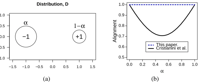
Figure 1: (a) Representation of the distribution D. In this simple two-dimensional example, a frac-tion αof the points are at (₋1,0) and have the label₋1. The remaining points are at

(1,0)and have the label+1. (b) Alignment values computed for two different definitions of alignment. The solid line in black plots the definition of alignment computed accord-ing to Cristianini et al. (2001) A= (α2_{+ (}₁₋_α₎2₎1/2_{, while our definition of centered}

alignment results in the straight dotted blue lineρ=1.

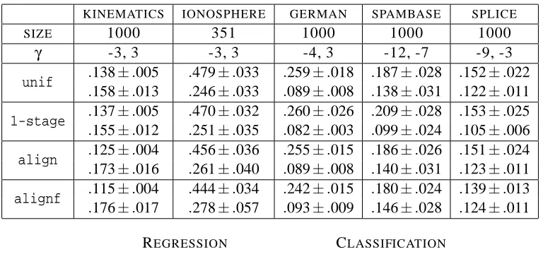
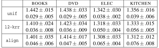
KINEMATICS IONOSPHERE GERMAN SPAMBASE SPLICE

(REGR.) (REGR.) (CLASS.) (CLASS.) (CLASS.)

b

ρ 0.9624 0.9979 0.9439 0.9918 0.9515

b

A 0.8627 0.9841 0.9390 0.9889 -0.4484

Table 1: The correlations of the alignment values and error-rates of various kernels. The top row re-ports the correlation of the accuracy of the base kernels used in Section 5 with the centered alignmentsbρ, the bottom row the correlation with the non-centered alignmentA.b

where the distribution D is defined by a fractionα_∈[0,1]of all points being at(₋1,0)and labeled with₋1, and the remaining points at(1,0)with label+1, as shown in Figure 1.

Clearly, for any value ofα_∈[0,1], the problem is separable, for example with the simple vertical line going through the origin, and one would expect the alignment to be 1. However, the alignment

A calculated using the definition of the distribution D admits a different expression. Using

E[K′2] =1,

E[K2] =α2_·₄_{+ (}₁₋_α₎2_·₄₊₂_α₍₁₋_α₎_·₀₌₄ _α2_{+ (}₁₋_α₎2_,

E[KK′] =α2_·₂_{+ (}₁₋_α₎2_·₂₊₂_α₍₁₋_α₎_·₀₌₂ _α2_{+ (}₁₋_α₎2_,

gives A= (α2_{+ (}₁₋_α₎2₎1/2_{. Thus, A is never equal to one except for}_α₌_{0 or}_α₌_{1 and for the}

balanced case whereα=1/2, its value is A=1/√2_≈.707<1. In contrast, with our definition,

ρ(K,K′) =1 for allα_∈[0,1](see Figure 1).

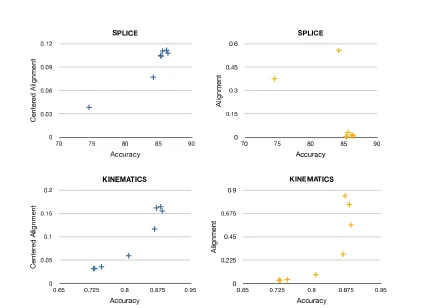
This mismatch between A (or A) and the performance values can also be seen in real worldb

(8)

Figure 2: Detailed view of the splice and kinematics experiments presented in Table 1. Both the centered (plots in blue on left) and non-centered alignment (plots in orange on right) are plotted as a function of the accuracy (for the regression problem in the kinematics task “accuracy” is 1 - RMSE). It is apparent from these plots that the non-centered alignment can be misleading when evaluating the quality of a kernel.

(2008) who have suggested various (input) data translation methods, and by Cristianini et al. (2002) who observed an issue for unbalanced data sets. Table 1, as well as Figure 2, give a series of empirical results in several classification and regression tasks based on data sets taken from the UCI Machine Learning Repository (http://archive.ics.uci.edu/ml/) and Delve data sets (http: //www.cs.toronto.edu/˜delve/data/datasets.html). The table and the figure illustrate the fact that the quantityA measured with respect to several different kernels does not always correlateb

well with the performance achieved by each kernel. In fact, for the splice classification task, the non-centered alignment is negatively correlated with the accuracy, while a large positive correlation is expected of a good quality measure. The centered notion of alignmentbρhowever, shows good correlation along all data sets and is always better correlated thanA.b

The notion of alignment seeks to capture the correlation between the random variables K(x,x′)

and K′(x,x′)and one could think it natural, as for the standard correlation coefficients, to consider the following definition:

ρ′₍_K_,_K′_{) =}_p E[(K−E[K])(K′−E[K′])]

(9)

However, centering the kernel values, as opposed to centering the feature values, is not directly relevant to linear predictions in feature space, while our definition of alignmentρis precisely related to that. Also, as already shown in Section 2.1, centering in the feature space implies the centering of the kernel values, since E[Kc] =0 and _m12∑_im_,_j₌₁[Kc]i j=0 for any kernel K and kernel matrix K.

Conversely, however, centering the kernel does not imply centering in feature space. For example, consider any kernel where all the row marginals are not all equal.

3. Algorithms

This section discusses several learning kernel algorithms based on the notion of centered alignment. In all cases, the family of kernels considered is that of non-negative combinations of p base kernels

Kk, k∈[1,p]. Thus, the final hypothesis learned belongs to the reproducing kernel Hilbert space

(RKHS)HKµ associated to a kernel of the form Kµ=∑

p

k=1µkKk, withµ≥0, which guarantees that

Kµis PDS, andkµk=Λ≥0, for some regularization parameterΛ.

We first describe and analyze two algorithms that both work in two stages: in the first stage, these algorithms determine the mixture weightsµ. In the second stage, they train a standard

kernel-based algorithm, for example, SVMs for classification, or KRR for regression, in combination with the kernel matrix Kµassociated to Kµ, to learn a hypothesis h∈HKµ. Thus, these two-stage

algo-rithms differ only by their first stage, which determines Kµ. We describe first in Section 3.1 a simple algorithm that determines each mixture weight µk independently, (align), then, in Section 3.2, an

algorithm that determines the weights µks jointly (alignf) by selectingµto maximize the alignment

with the target kernel. We briefly discuss in Section 3.3 the relationship of such two-stage learning algorithms with algorithms based on ensemble techniques, which also consist of two stages. Fi-nally, we introduce and analyze a single-stage alignment-based algorithm which learnsµand the

hypothesis h_∈HKµsimultaneously in Section 3.4.

3.1 Independent Alignment-based Algorithm (align)

This is a simple but efficient method which consists of using the training sample to independently compute the alignment between each kernel matrix Kk and the target kernel matrix KY =yy⊤,

based on the labels y, and to choose each mixture weight µk proportional to that alignment. Thus,

the resulting kernel matrix is defined by:

Kµ∝

p

∑

k=1

b

ρ(Kk,KY)Kk=

1

kKY_kF

p

∑

k=1

hKk,KYiF

kKk_kF

Kk. (3)

When the base kernel matrices Kk have been normalized with respect to the Frobenius norm, the

independent alignment-based algorithm can also be viewed as the solution of a joint maximization of the unnormalized alignment defined as follows, with a L2-norm constraint on the norm ofµ.

Definition 5 (Unnormalized alignment) Let K and K′be two PDS kernels defined over

X

_×

X

_and K and K′their kernel matrices for a sample of size m. Then, the unnormalized alignmentρu(K,K′)

between K and K′and the unnormalized alignmentρub(K,K′)between K and K′are defined by

ρu(K,K′) = E

x,x′[Kc(x,x

′₎_K′

c(x,x′)] and ρub(K,K′) =

1

(10)

Since they are not normalized, the alignment values a anda are no longer guaranteed to be in theb interval[0,1]. However, assuming the kernel function K and labels are bounded, the unnormalized alignment between K and KY are bounded as well.

Lemma 6 Let K be a PDS kernel. Assume that for all x_∈

X

_{, K}_c₍_x_,_x₎_≤_R2_{and for all output label} y,_|y_{| ≤}M. Then, the following bounds hold:

0_≤ρu(K,KY)≤MR2 and 0≤ρub(K,KY)≤MR2.

Proof The lower bounds hold by Lemma 3 and Inequality (2). The upper bounds can be obtained

straightforwardly via the application of the Cauchy-Schwarz inequality:

ρ2

u(K,KY) = E

(x,y),(x′_,_y′₎[Kc(x,x

′₎_yy′_]2_≤ _E x,x′[K

2

c(x,x′)]E y,y′[yy

′_]2_≤_R4_M2

b

ρu(K,K′) = 1

m2hKc,KYiF ≤

1

m2kKckFkKykF ≤

mR2mM m2 =R

2_M_,

where we used the identity_hKc,KY ciF =hKc,KYiF from Lemma 1.

We will consider more generally the corresponding optimization with an Lq-norm constraint onµ

with q>1:

max µ ρub

p

∑

k=1

µkKk,KY=D p

∑

k=1

µkKk,KYE

F (4)

subject to:

p

∑

k=1

µq_k ≤Λ.

An explicit constraint enforcingµ≥0 is not necessary since, as we shall see, the optimal solution

found always satisfies this constraint.

Proposition 7 Letµ∗be the solution of the optimization problem (4), then µ∗_k ∝hKk,KYi

1

q−1

F .

Proof The Lagrangian corresponding to the optimization (4) is defined as follows,

L(µ,β) =−

p

∑

k=1

µkhKk,KYiF+β( p

∑

k=1

µq_k₋Λ),

where the dual variableβis non-negative. Differentiating with respect to µkand setting the result to

zero gives

∂L ∂µk

=_−hKk,KYiF+qβµkq−1=0 =⇒ µk∝hKk,KYi

1

q−1

F ,

which concludes the proof.

Thus, for q=2, µk∝hKk,KYiF is exactly the solution given by Equation (3) modulo normalization

by the Frobenius norm of the base matrix. Note that for q=1, the optimization becomes trivial and can be solved by simply placing all the weight on µkwith the largest coefficient, that is the µkwhose

(11)

3.2 Alignment Maximization Algorithm

The independent alignment-based method ignores the correlation between the base kernel matrices. The alignment maximization method takes these correlations into account. It determines the mixture weights µk jointly by seeking to maximize the alignment between the convex combination kernel Kµ=∑

p

k=1µkKkand the target kernel KY=yy⊤.

This was also suggested in the case of uncentered alignment by Cristianini et al. (2001); Kandola et al. (2002a) and later studied by Lanckriet et al. (2004) who showed that the problem can be solved as a QCQP (however, as already discussed in Section 2.1, the uncentered alignment is not well correlated with performance). In what follows, we present even more efficient algorithms for computing the weights µk by showing that the problem can be reduced to a simple QP. We start by

examining the case of a non-convex linear combination where the components ofµcan be negative,

and show that the problem admits a closed-form solution in that case. We then partially use that solution to obtain the solution of the convex combination.

3.2.1 LINEARCOMBINATION

We can assume without loss of generality that the centered base kernel matrices Kkcare independent,

that is, no linear combination is equal to the zero matrix, otherwise we can select an independent subset. This condition ensures that_kKµ_ckF >0 for arbitraryµand thatbρ(Kµ,yy⊤)is well defined (Definition 4). By Lemma 1, _hKµ_c,KY ciF =hKµ_c,KYiF. Thus, sincekKY ckF does not depend

onµ, the alignment maximization problem max_µ_∈Mbρ(Kµ,yy⊤)can be equivalently written as the following optimization problem:

max µ∈M

hKµ_c,yy⊤iF

kKµ_ckF

, (5)

where

M

₌_{_µ_:_k_µ_k₂₌₁_}_{. A similar set can be defined via the L}₁_{-norm instead of L}₂_{. As we}

shall see, however, the direction of the solutionµ⋆ does not change with respect to the choice of

norm. Thus, the problem can be solved in the same way in both cases and subsequently scaled appropriately. Note that, by Lemma 1, Kµ_c=UmKµUmwith Um=I−11⊤/m, thus,

Kµ_c=Um

p

∑

k=1 µkKk

Um= p

∑

k=1

µkUmKkUm= p

∑

k=1 µkKkc.

Let

a= (_hK1c,yy⊤_iF, . . . ,hK_pc,yy⊤iF)⊤,

and let M denote the matrix defined by

Mkl=hKkc,Kl ciF,

(12)

symmetric PSD matrix since for any vector X= (x1, . . . ,xp)⊤∈Rp, X⊤MX=

p

∑

k,l=1

xkxlMkl

=Trh

p

∑

k,l=1

xkxlKkcKl c

i

=Trh( p

∑

k=1

xkKkc)( p

∑

l=1 xlKl c)

i

=_k p

∑

k=1

xkKkc_k2_F>0.

The strict inequality follows from the fact that the base kernels are linearly independent. Since this inequality holds for any non-zero X, it also shows that M is invertible.

Proposition 8 The solutionµ⋆of the optimization problem (5) is given byµ⋆= M−

1_a

kM−1_a_k.

Proof With the notation introduced, problem (5) can be rewritten asµ⋆=argmax_k_µ_k₂₌₁ µ

⊤_a

√

µ⊤Mµ .

Thus, clearly, the solution must verifyµ⋆⊤a≥0. We will square the objective and yet not enforce

this condition since, as we shall see, it will be verified by the solution we find. Therefore, we consider the problem

µ⋆=argmax

kµk2=1

(µ⊤a)2

µ⊤Mµ =argmax_k_µ_k₂₌₁

µ⊤aa⊤µ

µ⊤Mµ .

In the final equality, we recognize the general Rayleigh quotient. Letν=M1/2µandν⋆=M1/2µ⋆,

then

ν⋆= argmax

kM−1/2_ν_k 2=1

ν⊤M−1/2aa⊤M−1/2ν

ν⊤ν .

Hence, the solution is

ν⋆= argmax

kM−1/2

νk2=1

ν⊤M−1/2a2

kνk2₂

= argmax

kM−1/2

νk2=1

ν

kνk

_⊤

M−1/2a

2 .

Thus,ν⋆∈Vec(M−1/2a)withkM−1/2ν⋆k2=1. This yields immediatelyµ⋆= M−

1_a

kM−1_a_k, which

ver-ifiesµ⋆⊤a=a⊤M−1a/kM−1ak ≥0 since M and M−1are PSD.

3.2.2 CONVEXCOMBINATION(alignf)

In view of the proof of Proposition 8, the alignment maximization problem with the set

M

′ ₌ {kµk2=1∧µ≥0}can be written as

µ∗=argmax µ∈M′

µ⊤aa⊤µ

µ⊤Mµ. (6)

(13)

Proposition 9 Let v⋆be the solution of the following QP:

min

v≥0v

⊤_Mv₋_2v⊤_a. ₍₇₎

Then, the solutionµ∗of the alignment maximization problem (6) is given byµ⋆=v⋆/kv⋆k.

Proof Note that problem (7) is equivalent to the following one defined overµand b

min µ≥0,kµk2=1

b>0

b2µ⊤Mµ−2bµ⊤a, (8)

where the relation v=bµcan be used to retrieve v. The optimal choice of b as a function ofµ

can be found by setting the gradient of the objective function with respect to b to zero, giving the closed-form solution b∗= µ⊤a

µ⊤Mµ. Plugging this back into (8) results in the following optimization after straightforward simplifications:

min µ≥0,kµk2=1

−(µ⊤a)

2

µ⊤Mµ,

which is equivalent to (6). This shows that v⋆=b∗µ∗whereµ∗is the solution of (6) and concludes

the proof.

It is not hard to see that this problem is equivalent to solving a hard margin SVM problem, thus, any SVM solver can also be used to solve it. A similar problem with the non-centered definition of alignment is treated by Kandola et al. (2002b), but their optimization solution differs from ours and requires cross-validation.

Also, note that solving this QP problem does not require a matrix inversion of M. In fact, the assumption about the invertibility of matrix M is not necessary and a maximal alignment solution can be computed using the same optimization as that of Proposition 9 in the non-invertible case. The optimization problem is then not strictly convex however and the alignment solutionµnot unique.

We now further analyze the properties of the solution v of problem (7). Letbρ0(µ)denote the

partially normalized alignment maximized by (5):

b

ρ0(µ) =kyy⊤k2_Fbρ(µ) =hKµc,yy

⊤_i_F

kKµ_ckF

=pµ⊤a µ⊤Mµ

=hµ,M− 1_a_i

M

p µ⊤Mµ

= hµ,M− 1_a_i

M

kµkM

.

The following proposition gives a simple expression forbρ0(µ).

Proposition 10 Forµ=v/kvk, with v6=0 solution of the alignment maximization problem (7), the

following identity holds:

b

ρ0(µ) =kvkM.

Proof Since_kv_k2_M₋2v⊤a=_kv_k2_M₋2_hv,M−1_a_i

M=kv−M−1ak2_M− kM−1ak2_M the optimization problem (7) can be equivalently written as

min

v≥0kv−M

−1_a_k2

(14)

This implies that the solution v is the M-orthogonal projection of M−1a over the convex set{v : v≥

0_}. Therefore, v₋M−1a is M-orthogonal to v:

hv,v₋M−1a_iM=0 =⇒ kvk2M=hv,M−1aiM.

Thus,

kv_kM=h

v,M−1_a_i

M

kv_kM

=hµ,M− 1_a_i

M

kµkM

=ρ(µ),

Thus, the proposition gives a straightforward way of computingρ0(µ), thereby alsoρ(µ), from the

M-norm of the solution vector v thatµis derived from.

3.3 Relationship with Ensemble Techniques

An alternative two-stage technique for learning with multiple kernels consists of first learning a pre-diction hypothesis hk using each kernel Kk, k∈[1,p], and then of learning the best linear

combina-tion of these hypotheses: h=∑_kp₌₁µkhk. But, such ensemble-based techniques make use of a richer

hypothesis space than the one used by learning kernel algorithms such as that of Lanckriet et al. (2004). For ensemble techniques, each hypothesis hk, k∈[1,p], is of the form hk=∑mi=1αikKk(xi,·)

for some αk = (α1k, . . . ,αmk)⊤∈Rm with different constraintskαkk ≤Λk, Λk ≥0, and the final

hypothesis is of the form

p

∑

k=1 µkhk=

p

∑

k=1 µk

m

∑

j=1

αikKk(xi,·) = m

∑

i=1 p

∑

k=1

µkαikKk(xi,·).

In contrast, the general form of the hypothesis learned using kernel learning algorithms is

m

∑

i=1

αiKµ(xi,·) =

m

∑

i=1 αi

∑

p

k=1

µkKk(xi,·) = p

∑

k=1 m

∑

i=1

µkαiKk(xi,·),

for some α∈Rm with kαk ≤Λ, Λ ≥0. When the coefficients αik can be decoupled, that is

αik=αiβkfor someβks, the two solutions seem to have the same form but they are in fact different since in general the coefficients must obey different constraints (differentΛks). Furthermore, the combination weights µi are not required to be positive in the ensemble case. We present a more

detailed theoretical and empirical comparison of the ensemble and learning kernel techniques else-where (Cortes et al., 2011a).

3.4 Single-stage Alignment-based Algorithm

This section analyzes an optimization based on the notion of centered alignment, which can be viewed as the single-stage counterpart of the two-stage algorithm discussed in Sections 3.1 - 3.2.

As in Sections 3.1 and 3.2, we denote by a the vector(_hK1c,yy⊤_iF, . . . ,hK_pc,yy⊤iF)⊤and let M_∈Rp×p be the matrix defined by Mkl=hKkc,Kl ciF. The optimization is then defined by

aug-menting standard single-stage learning kernel optimizations with an alignment maximization con-straint. Thus, the domain

M

_{of the kernel combination vector}_µ_{is defined by:}

(15)

for non-negative parametersΛandΩ. The alignment constraintρ(Kµ,yy⊤)≥Ωcan be rewritten asΩpµ⊤Mµ−µ⊤a≤0, which defines a convex region. Thus,

M

is a convex subset ofRp.

For a fixedµ∈

M

and corresponding kernel matrix Kµ, let F(µ,α)denote the objective func-tion of the dual optimizafunc-tion problem minimizeα∈AF(µ,α)solved by an algorithm such as SVM, KRR, or more generally any other algorithm for which

A

_{is a convex set and F}₍_µ_,_·₎ _{a concave}

function for allµ∈

M

, and F(·,α)convex for allα∈

A

. Then, the general form of a single-stage

alignment-based learning kernel optimization is

min µ∈M

max α∈A

F(µ,α).

Note that, by the convex-concave properties of F and the convexity of

M

_and

A

_{, von Neumann’s}

minimax theorem applies:

min µ∈M

max α∈A

F(µ,α) =max α∈A

min µ∈M

F(µ,α).

We now further examine this optimization problem in the specific case of the kernel ridge regression algorithm. In the case of KRR, F(µ,α) =−α⊤(Kµ+λI)α+2α⊤y. Thus, the max-min problem can be rewritten as

max α∈A

min µ∈M−

α⊤(Kµ+λI)α+2α⊤y.

Let bαdenote the vector(α⊤K1α, . . . ,α⊤Kpα)⊤, then the problem can be rewritten as

max α∈A−

λα⊤α+2α⊤y−max µ∈M

µ⊤bα,

where λ =λ0m in the notation of Equation (10). We first focus on analyzing only the term −max_µ_∈Mµ⊤bα. Since the last constraint in

M

is convex, standard Lagrange multiplier theory guarantees that for anyΩthere exists aγ_≥0 such that the following optimization is equivalent to the original maximization overµ.

min

µ −

µ⊤bα+γ(Ω p

µ⊤Mµ−µ⊤a)

subject toµ≥0∧ kµk ≤Λ∧γ≥0.

Note thatγis not a variable, but rather a parameter that will be hand-tuned. Now, again applying standard Lagrange multiplier theory we have that for any(γΩ)_≥0 there exists anΩ′ such that the following optimization is equivalent:

min ₋µ⊤(γa+bα)

subject toµ≥0∧ kµk ≤Λ∧γ≥0∧µ⊤Mµ≤Ω′2.

Applying the Lagrange technique a final time (for anyΛthere exists aγ′_≥0 and for anyΩ′2there exists aγ′′_≥0) leads to

(16)

This is a simple QP problem. Note that the overall problem can now be written as

max α∈A,µ≥0−

λα⊤α+2α⊤y+µ⊤(γa+bα)−γ′µ⊤µ−γ′′µ⊤Mµ.

This last problem is not convex in(α,µ), but the problem is convex in each variable. In the case

of kernel ridge regression, the maximization inα admits a closed form solution. Plugging in that

solution yields the following convex optimization problem inµ:

min µ≥0y

⊤₍_K

µ+λI)−

1_y

−γµ⊤a+µ⊤(γ′′M+γ′I)µ.

Note that multiplying the objective by λ using the substitution µ′= _λ1µresults in the following

equivalent problem,

min µ′≥0y

⊤₍_K

µ′+I)−

1_y₋_λ2_γ

µ′⊤a+µ′⊤(λ3γ′′M+λ3γ′I)µ′,

which makes clear that the trade-off parameterλcan be subsumed by theγ,γ′ andγ′′parameters. This leads to the following simpler problem with a reduced number of trade-off parameters,

min µ≥0

y⊤(Kµ+I)−

1_y₋_γ

µ⊤a+µ⊤(γ′′M+γ′I)µ. (9)

This is a convex optimization problem. In particular, µ7→y⊤(Kµ+I)−1y is a convex funtion by convexity of f : M_7→y⊤M−1y over the set of positive definite symmetric matrices. The convexity

of f can be seen from that of its epigraph, which, by the property of the Schur complement, can be written as follows (Boyd and Vandenberghe, 2004):

epi f=_{(M,t): M_≻0,y⊤M−1y_≤t_}=_{(M,t):

M y y⊤ t

0,M_≻0_}.

This defines a linear matrix inequality in(M,t)and thus a convex set. The convex optimization (9) can be solved efficiently using a simple iterative algorithm as in Cortes et al. (2009a). In practice, the algorithm converges within 10-50 iterations.

4. Theoretical Results

This section presents a series of theoretical guarantees related to the notion of kernel alignment. Section 4.1 proves a concentration bound of the form_|ρ₋bρ| ≤O(1/√m), which relates the centered alignmentρto its empirical estimatebρ. In Section 4.2, we prove the existence of accurate predictors in both classification and regression in the presence of a kernel K with good alignment with respect to the target kernel. Section 4.3 presents stability-based generalization bounds for the two-stage alignment maximization algorithm whose first stage was described in Section 3.2.2.

4.1 Concentration Bounds for Centered Alignment

Our concentration bound differs from that of Cristianini et al. (2001) both because our definition of alignment is different and because we give a bound directly on the quantity of interest_|ρ₋bρ|. Instead, Cristianini et al. (2001) give a bound on _|A′₋Ab_|, where A′ ₆=A can be related to A by

replacing each Frobenius product with its expectation over samples of size m.

(17)

Proposition 11 Let K and K′ denote kernel matrices associated to the kernel functions K and K′ for a sample of size m drawn according to D. Assume that for any x_∈

X

_{, K}₍_x_,_x₎_≤_R2 _and K′(x,x)_≤R′2. Then, for anyδ>0, with probability at least 1₋δ, the following inequality holds:

h

Kc,K′ciF

m2 −E[KcKc′]

≤

18R2_R′2 m +24R

2_R′2

s log2_δ

2m .

Note that in the case K′(xi,xj) =yiyj, we then have R′2≤maxiy2i.

Proof The proof relies on a series of lemmas given in the Appendix. By the triangle inequality and

in view of Lemma 19, the following holds:

h

Kc,K′ciF

m2 −E[KcKc′]

≤ h

Kc,K′ciF m2 −E

hKc,K′ciF

m2

+

18R2R′2

m .

Now, in view of Lemma 18, the application of McDiarmid’s inequality (McDiarmid, 1989) to

hKc,K′ciF

m2 gives for anyε>0:

PrhKc,K′ciF

m2 −E

hKc,K′ciF

m2

>ε

≤2 exp[₋2mε2/(24R2R′2)2_]_.

Settingδto be equal to the right-hand side yields the statement of the proposition.

Theorem 12 Under the assumptions of Proposition 11, and further assuming that the conditions of the Definitions 2-4 are satisfied forρ(K,K′)andbρ(K,K′₎_{, for any}_δ_>_{0, with probability at least}

1₋δ, the following inequality holds:

|ρ(K,K′)₋bρ(K,K′)_{| ≤}18β

" 3

m+8

s log6_δ

2m #

,

withβ=max(R2R′2/E[K_c2],R2R′2/E[K_c′2]).

Proof To shorten the presentation, we first simplify the notation for the alignments as follows:

ρ(K,K′) =_√b

aa′ bρ(K,K

′_{) =}_√bb

b

aa_b′,

with b=E[KcKc′], a=E[Kc2], a′=E[Kc′2]and similarly,bb= (1/m2)hKc,K′ciF, ba= (1/m2)kKck2,

anda_b′= (1/m2)_kK′_c_k2. By Proposition 11 and the union bound, for anyδ>0, with probability at least 1₋δ, all three differences a₋_ba, a′₋_ba′, and b₋b are bounded byb α=18R_m2R′2+24R2R′2

q

log6_δ 2m .

Using the definitions ofρandbρ, we can write:

|ρ(K,K′)₋bρ(K,K′)_|=√b

aa′−

bb √

b

aa_b′

=b

√

b

a_ba′₋bb√aa′ √

aa′_a_b_a_b′

=(b−bb)

√

b

aa_b′₋b_b₍√_aa′₋√_a_b_a_b′₎ √

aa′a_ba_b′

=(b_√−bb)

aa′ −bρ(K,K

′₎_√ aa′−abba′ aa′₍√_aa′₊√_a_b_a_b′₎

(18)

Sincebρ(K,K′₎_∈_[₀_,₁_]_{, it follows that}

|ρ(K,K′)₋bρ(K,K′)_{| ≤} |b√−bb|

aa′ +

|aa′₋a_ba_b′_|

√

aa′₍√_aa′₊√_b_a_a_b′₎.

Assume first that a_b_≤a_b′. Rewriting the right-hand side to make the differences a₋a and a_b ′₋a_b′

appear, we obtain:

|ρ(K,K′)₋bρ(K,K′)_{| ≤} |b_√−bb|

aa′ +

|(a₋_ba)a′+_ba(a′₋_ba′)_|

√

aa′(√aa′+√a_ba_b′)

≤√α

aa′

1+√ a′+ba aa′₊√_a_b_a_b′

≤√α

aa′

1+√a′

aa′+

b

a √

b

aa_b′

≤√α

aa′

" 2+

r

a′ a

#

=

2

√ aa′ +

1

a

α.

We can similarly obtainh√2 aa′+

1 a′ i

αwhen_ba′_≤a. Both bounds are less than or equal to 3 max_b (α_a,_aα′).

Equivalently, one can set the right hand side of the high probability statement presented in Theo-rem 12 equal toεand solve forδ, which shows that Pr_|ρ(K,K′)₋bρ(K,K′)_|>ε_≤O(e−mε2).

4.2 Existence of Good Alignment-based Predictors

For classification and regression tasks, the target kernel is based on the labels and defined by

KY(x,x′) =yy′, where we denote by y the label of point x and y′ that of x′. This section shows

the existence of predictors with high accuracy both for classification and regression when the align-mentρ(K,KY)between the kernel K and KY is high.

In the regression setting, we shall assume that the labels have been normalized such that E[y2] =

1. In classification, y=_±1 and thus E[y2] =1 without any normalization. Denote by h∗the hypoth-esis defined for all x_∈

X

_by

h∗(x) =Ex′p[y′Kc(x,x′)] E[K2

c] .

Observe that by definition of h∗, Ex[yh∗(x)] =ρ(K,KY). For any x∈

X

, defineγ(x) =

r

Ex′[Kc2(x,x′)]

Ex,x′[Kc2(x,x′)] andΓ=maxxγ(x). The following result shows that the hypothesis h∗has high accuracy when the

kernel alignment is high andΓnot too large.3

Theorem 13 (classification) Let R(h∗) =Pr[yh∗(x)<0]denote the error of h∗in binary classifica-tion. For any kernel K such that 0<E[K_c2]<+∞, the following holds:

R(h∗)_≤1₋ρ(K,KY)/Γ.

3. A version of this result was presented by Cristianini, Shawe-Taylor, Elisseeff, and Kandola (2001) and Cristianini, Kandola, Elisseeff, and Shawe-Taylor (2002) for the so-called Parzen window solution and non-centered kernels.

However, both proofs are incorrect since they rely implicitly on the fact that maxx

E_x′[K2₍_x,x′)]

Ex,x′[K2₍_x,x′_)]

1

2₌_{1, which can}

only hold in the trivial case where the kernel function K2is a constant: by definition of the maximum and expectation operators, maxx

Ex′[K2(x,x′)]≥Ex

(19)

Proof Note that for all x∈

X

_,

|yh∗(x)_|=|y Ex_p′[y′Kc(x,x′)]|

E[K2 c]

≤

p

Ex′[y′2]E_x′[K_c2(x,x′)] p

E[K2 c]

=

p

Ex′[K_c2(x,x′)] p

E[K2 c]

≤Γ.

In view of this inequality, and the fact that Ex[yh∗(x)] =ρ(K,KY), we can write:

1−R(h∗) =Pr[yh∗(x)_≥0] =E[1_{_yh∗₍_x₎_≥₀_}]

≥E

yh∗(x)

Γ 1{yh∗(x)≥0}

≥E

yh∗(x) Γ

=ρ(K,KY)/Γ,

where 1_ωis the indicator function of the eventω.

A probabilistic version of the theorem can be straightforwardly derived by noting that by Markov’s inequality, for anyδ>0, with probability at least 1₋δ,_|γ(x)_{| ≤}1/√δ.

Theorem 14 (regression) Let R(h∗) =Ex[(y−h∗(x))2]denote the error of h∗ in regression. For any kernel K such that 0<E[K_c2]<+∞, the following holds:

R(h∗)_≤2(1₋ρ(K,KY)). Proof By the Cauchy-Schwarz inequality, it follows that:

E

x[h ∗2

(x)] =E

x

Ex′[y′Kc(x,x′)]2

E[K2 c]

≤E

x

Ex′[y′2]E_x′[K_c2(x,x′)] E[K2

c]

=Ex′[y′ 2_]_E

x,x′[K_c2(x,x′)] E[K2

c]

=E

x′[y

′2_{] =}₁_.

Using again the fact that Ex[yh∗(x)] =ρ(K,KY), the error of h∗can be bounded as follows:

E[(y₋h∗(x))2_{] =}_E x[h

∗₍_x₎2_{] +}_E x[y

2_]₋_{2 E} x[yh

∗₍_x_)]_≤₁₊₁₋₂_ρ₍_K_,_K Y),

The hypothesis h∗ is closely related to the hypothesis h∗_S derived as follows from a finite sample

S= ((x1,y1), . . . ,(xm,ym)): hS(x) =

1 m∑

m

i=1yiKc(x,xi)

q

1 m2∑

m

i,j=1Kc(xi,xj)2

q

1 m2∑

m

i,j=1(yiyj)2 .

(20)

For classification, the existence of a good predictor g∗based on the unnormalized alignmentρu (see Definition 5) can also be shown. The corresponding guarantees are simpler and do not depend on a term such asΓ. However, unlike the normalized case, the loss of the predictor g∗_Sderived from a finite sample may not always be close to that of g∗. Note that in classification, for any label y,

|y_|=1, thus, by Lemma 6, the following holds: 0_≤ρu(K,KY)| ≤R2. Let g∗ be the hypothesis

defined by:

g∗(x) =E

x′[y

′_K

c(x,x′)].

Since 0≤ρu(K,KY)| ≤R2, the following theorem provides strong guarantees for g∗ when the

un-normalized alignment a is sufficiently large, that is close to R2.

Theorem 15 (classification) Let R(g∗) =Pr[yg∗(x)<0]denote the error of g∗in binary classifica-tion. For any kernel K such that sup_x_∈XKc(x,x)≤R2, we have:

R(g∗)_≤1₋ρu(K,KY)/R2. Proof Note that for all x_∈

X

_,

|yg∗(x)_|=_|g∗(x)_|=_|E

x′[y

′_K

c(x,x′)]| ≤R2.

Using this inequality, and the fact that Ex[yg∗(x)] =ρu(K,KY), we can write:

1₋R(g∗) =Pr[yg∗(x)_≥0] =E[1_{_yg∗₍_x₎_≥₀_}]

≥E

yg∗(x)

R2 1{yh∗(x)≥0}

≥E

yg∗(x)

R2

=ρu(K,KY)/R2,

4.3 Generalization Bounds for Two-stage Learning Kernel Algorithms

This section presents stability-based generalization bounds for two-stage learning kernel algorithms. The proof of a stability-based learning bound hinges on showing that the learning algorithm is

sta-ble, that is the pointwise loss of a learned hypothesis does not change drastically if the training

sample changes only slightly. We refer the reader to Bousquet and Elisseeff (2000) for a full intro-duction.

(21)

Recall that for a fixed kernel function Kµ with associated RKHS HKµ and training set S=

((x1,y1), . . . ,(xm,ym)), the KRR optimization problem is defined by the following constraint

opti-mization problem:

min

h∈HKµ

G(h) =λ0_khk2 Kµ+

1

m m

∑

i=1

(h(xi)−yi)2. (10)

We first analyze the stability of two-stage algorithms and then use that to derive a stability-based generalization bound (Bousquet and Elisseeff, 2000). More precisely, we examine the pointwise difference in hypothesis values obtained on any point x when the algorithm has been trained on two data sets S and S′ of size m that differ in exactly one point.

In what follows, we denote by_kK_ks,t= (∑_kp₌₁kKkkts)1/t the(s,t)-norm of a collection of

matri-ces and by∆µthe differenceµ′−µof the combination vectorµ′ andµreturned by the first stage

of the algorithm by training on S, respectively S′.

Theorem 16 (Stability of two-stage learning kernel algorithm) Let S and S′ be two samples of size m that differ in exactly one point and let h and h′ be the associated hypotheses generated by a two-stage KRR learning kernel algorithm with the constraintµ∈

M

1. Then, for any s,t≥1 with

1 s+

1

r =1 and any x∈

X

:

|h′(x)₋h(x)_{| ≤}2Λ1R

2_M λ0m

h

1+k∆µkskKck2,t

2λ0 i

,

where M is an upper bound on the target labels and R2=supk∈[1,p]

x∈X

Kk(x,x).

Proof The KRR algorithm returns the hypothesis h(x) = ∑m

i=1αiKµ(xi,x), where α= (Kµ+

mλ0I)−1_{y. Thus, this hypothesis is parametrized by the kernel weight vector}_µ_{, which defines the}

kernel function, and the sample S, which is used to populate the kernel matrix, and will be explicitly denoted hµ,S. To estimate the stability of the overall two-stage algorithm,∆hµ,S=hµ′,S′−hµ,S, we use the decomposition

∆hµ,S= (hµ′,S′−hµ′,S) + (hµ′,S−hµ,S)

and bound each parenthesized term separately. The first parenthesized term measures the point-wise stability of KRR due to a change of a single training point with a fixed kernel. This can be bounded using Theorem 2 of Cortes et al. (2009a). Since, for all x_∈

X

_{, K}_µ₍_x_,_x_{) =}∑p

k=1µkKk(x,x)≤ R2∑_kp₌₁µk≤Λ1R2, using that theorem yields the following bound:

∀x∈

X

_, _|_h

µ,S′(x)−hµ,S(x)| ≤

2Λ1R2_M λ0m .

The second parenthesized term measures the pointwise difference of the hypotheses due to the change of kernel from Kµ′ to Kµfor a fixed training sample when using KRR. By Proposition 1 of Cortes et al. (2010c), this term can be bounded as follows:

∀x∈

X

_,_|_h

µ′,S(x)−hµ,S(x)| ≤

Λ1R2_M λ2

0m

kKµ′−Kµk.

The term_kKµ′−Kµkcan be bounded using H¨older’s inequality as follows:

kKµ′−Kµk=k

p

∑

k=1

(∆µk)Kkk ≤ p

∑

k=1