A Multi-Stage Framework for Dantzig Selector and LASSO

(1)

A Multi-Stage Framework for Dantzig Selector and LASSO

Arizona State University 699 South Mill Avenue Tempe, AZ 85287-8809, USA

Editor: Tong Zhang

Abstract

We consider the following sparse signal recovery (or feature selection) problem: given a design matrix X _∈Rn×m_(m_≫_n)_{and a noisy observation vector y}_∈Rn _{satisfying y}₌_Xβ∗₊_ε_where

εis the noise vector following a Gaussian distribution N(0,σ2_{I), how to recover the signal (or}

parameter vector)β∗when the signal is sparse?

The Dantzig selector has been proposed for sparse signal recovery with strong theoretical guar-antees. In this paper, we propose a multi-stage Dantzig selector method, which iteratively refines the target signalβ∗. We show that if X obeys a certain condition, then with a large probability the difference between the solution ˆβestimated by the proposed method and the true solutionβ∗ measured in terms of theℓpnorm (p≥1) is bounded as

kβˆ−β∗kp≤

C(s−N)1/pp

log m+∆σ,

where C is a constant, s is the number of nonzero entries inβ∗, the risk of the oracle estimator∆is independent of m and is much smaller than the first term, and N is the number of entries ofβ∗larger than a certain value in the order ofO₍σ√_{log m). The proposed method improves the estimation} bound of the standard Dantzig selector approximately from Cs1/p√log mσto C(s−N)1/p√_{log m}_σ

where the value N depends on the number of large entries in β∗. When N=s, the proposed algorithm achieves the oracle solution with a high probability, where the oracle solution is the projection of the observation vector y onto true features. In addition, with a large probability, the proposed method can select the same number of correct features under a milder condition than the Dantzig selector. Finally, we extend this multi-stage procedure to the LASSO case.

Keywords: multi-stage, Dantzig selector, LASSO, sparse signal recovery

1. Introduction

(2)

equivalent to feature selection (or model selection). In feature selection, one concerns the feature selection accuracy. Typically, a group of features corresponding to the coefficient values in ˆβ larger than a threshold form the supporting feature set. The difference between this set and the true supporting set (i.e., the set of features corresponding to nonzero coefficients in the original signal) measures the feature selection accuracy.

Two well-known algorithms for learning sparse signals include LASSO (Tibshirani, 1996) and Dantzig selector (Cand`es and Tao, 2007):

LASSO min

β : 1

2kXβ−yk 2

2+λ′||β||1, Dantzig Selector min

β :||β||1

s.t.:_kXT(Xβ₋y)_k_∞_≤λ.

Strong theoretical results concerning LASSO and Dantzig selector have been established in the literature (Cai et al., 2009; Cand`es and Plan, 2009; Cand`es and Tao, 2007; Wainwright, 2009; Zhang, 2009a; Zhao and Yu, 2006).

1.1 Contributions

In this paper, we propose a multi-stage procedure based on the Dantzig selector, which estimates the supporting feature set F0and the signal ˆβiteratively. The intuition behind the proposed multi-stage method is that feature selection and signal recovery are tightly correlated and they can benefit from each other: a more accurate estimation of the supporting features can lead to a better signal recovery and a more accurate signal recovery can help identify a better set of supporting features. In the proposed method, the supporting set F0starts from an empty set and its size increases by one after each iteration. At each iteration, we employ the basic framework of Dantzig selector and the information about the current supporting feature set F0to estimate the new signal ˆβ. In addition, we select the supporting feature candidates in F0 among all features in the data at each iteration, thus allowing to remove incorrect features from the previous supporting feature set.

The main contributions of this paper lie in the theoretical analysis of the proposed method. Specifically, we show: 1) the proposed method can improve the estimation bound of the standard Dantzig selector approximately from Cs1/p√log mσto C(s₋N)1/p√_{log m}_σ_{where the value N}

de-pends on the number of large entries inβ∗; 2) when N=s, the proposed algorithm can achieve the

oracle solution ¯βwith a high probability, where the oracle solution is the projection of the observa-tion vector y onto true features (see Equaobserva-tion (1) for the explicit descripobserva-tion of ¯β); 3) with a high probability, the proposed method can select the same number of correct features under a milder condition than the standard Dantzig selector method; 4) this multi-stage procedure can be easily extended to the LASSO case. The numerical experiments validate these theoretical results.

1.2 Related Work

(3)

is strong enough together with some additional assumptions on its supporting set and signs, the mutual incoherence property (MIP) (or incoherence condition) can guarantee the feature selection consistency and the sign consistency with a high probability. A comprehensive analysis for LASSO, including the recovery accuracy in an arbitraryℓpnorm (p≥1) and the feature selection consistency,

was presented in Zhang (2009a). Cand`es and Tao (2007) proposed the Dantzig selector (which is a linear programming problem) for sparse signal recovery and presented a bound of recovery accuracy with the same order as LASSO under the uniform uncertainty principle (UUP). An approximate equivalence between the LASSO estimator and the Dantzig selector was given by Bickel et al. (2009). Lounici (2008) studied the ℓ_∞ convergence rate for LASSO and Dantzig estimators in a high-dimensional linear regression model under MIP. James et al. (2009) provided conditions on the design matrix X under which the LASSO and Dantzig selector coefficient estimates are identical for certain tuning parameters. Please refer to recent papers (Zhang, 2009a; Fan and Lv, 2010) for a more comprehensive overview of LASSO and Dantzig selector.

Since convex regularization methods like LASSO and Dantzig selector give biased estimation due to convex regularization, many heuristic methods have been proposed to correct the bias of convex relaxation recently, including orthogonal matching pursuit (OMP) (Tropp, 2004; Donoho et al., 2006; Zhang, 2009b, 2011a; Cai and Wang, 2011), two stage LASSO (Zhang, 2009a), multi-ple thresholding LASSO (Zhou, 2009), adaptive LASSO (Zou, 2006), adaptive forward-backward greedy method (FoBa) (Zhang, 2011b), and nonconvex regularization methods (Zhang, 2010b; Fan and Lv, 2011; Lv and Fan, 2009; Zhang, 2011b). They have been shown to outperform the standard convex methods in many practical applications. It was shown that under exact recovery condition (ERC) (similar to MIP) the solution of OMP guarantees the feature selection consistency in the noiseless case (Tropp, 2004). The results of Tropp (2004) were extended to the noisy case by Zhang (2009b). Very recently, Zhang (2011a) showed that under RIP (weaker than MIP and ERC), OMP can stably recover a sparse signal in 2-norm under measurement noise. A multiple thresholding pro-cedure was proposed to refine the solution of LASSO or Dantzig selector (Zhou, 2009). The FoBa algorithm was proposed by Zhang (2011b), and it was shown that under RIP the feature selection consistency is achieved if the minimal nonzero entry in the true solution is larger than

O

₍σ√_{log m}₎_.

The adaptive LASSO was proposed to adaptively tune the weight value for theℓ1 norm penalty, and it was shown to enjoy the oracle properties (Zou, 2006). Zhang (2010b) proposed a general multi-stage convex regularization method (MSCR) to solve a nonconvex sparse regularization prob-lem. It was also shown that a specific case “least square loss + nonconvex sparse regularization” can eliminate the bias in signal recovery (Zhang, 2010b) and achieve the feature selection con-sistency (Zhang, 2011c) under the sparse eigenvalue condition (SEC) if the true signal is strong enough. More related work about nonconvex regularization methods can be found in a recent paper by Zhang and Zhang (2012).

Conditions mentioned above can be classified into two classes: 1) theℓ2 conditions including RIP, UUP, and SEC; 2) the ℓ_∞ conditions including ERC and MIP. Overall, the ℓ2 conditions are considered to be weaker than theℓ∞ conditions, since theℓ∞conditions require about

O

₍_s2_{log m}₎

random projections while theℓ2conditions only need

O

(s log m)random projections. 1.3 Definitions, Notations, and Basic Assumptions

We use X _∈Rn×m _{to denote the design matrix and focus on the case m}_≫_{n, that is, the signal}

(4)

A=XTX with respect to the design matrix. The noise vector ε follows the multivariate normal distributionε∼_N₍₀_,σ2_I₎_{. The observation vector y}_∈Rn _{satisfies y}₌_Xβ∗₊ε_{, where}β∗_denotes

the original signal (or true solution). ˆβis used to denote the solution of the proposed algorithm. The

α-supporting set (α≥0) for a vectorβis defined as

suppα(β) =_{j : _|βj|>α}.

The “supporting” set of a vector refers to the 0-supporting set. F denotes the supporting set of the original signalβ∗. For any index set S,_|S_|denotes the size of the set and ¯S denotes the complement

of S in_{1,2,3, ...,m_}. In this paper, s is used to denote the size of the supporting set F, that is,

s=_|F_|. We useβSto denote the subvector ofβconsisting of the entries ofβin the index set S. The

ℓpnorm of a vector v is computed bykvkp= (∑i|vi|p)1/p, where videnotes the ith entry of v. The

oracle solution ¯βis defined as

¯

βF = (X_FTXF)−1XFTy and ¯βF¯ =0. (1)

We employ the following notation to measure some properties of a PSD matrix M_∈RK×K _(Zhang,

2009a):

µ(_Mp_,)_k = inf

u∈Rk_,_|_I_|₌_k

kMI,Iukp

ku_kp

, ρ(_Mp_,)_k= sup

u∈Rk_,_|_I_|₌_k

kMI,Iukp

ku_kp

,

θ(p)

M,k,l = sup

u∈Rl_,_|_I_|₌_k_,_|_J_|₌_l_,_I_∩_J₌∅

kMI,Jukp

ku_kp

, γM=max

i6=j |Mi j|,

where p_∈[1,∞], I and J are disjoint subsets of_{1,2, ...,K_}, and MI,J ∈R|I|×|J| is a submatrix of

M with rows from the index set I and columns from the index set J. One can easily verify that µ(∞)_A_,_k _≥1₋γA(k₋1),ρ(∞)_A_,_k _≤1+γA(k₋1), andθ(∞)_A_,_k_,_l _≤lγA, if all columns of X are normalized to have a unit length.

Additionally, we use the following notation to denote two probabilities:

η′

1=η1(πlog((m−s)/η1))−1/2, η′2=η2(πlog(s/η2))−1/2,

whereη1 andη2are two factors between 0 and 1. In this paper, if we say “large”, “larger” or “the largest”, it means that the absolute value is large, larger or the largest. For simpler notation in the computation of sets, we sometimes use “S1+S2” to indicate the union of two sets S1 and S2, and use “S1−S2” to indicate the removal of the intersection of S1 and S2 from the first set S1. In this paper, the following assumption is always admitted.

Assumption 1 We assume that s=_|supp0(β∗)|<n, the variable number is much larger than the

feature dimension (i.e., m_≫n), each column vector is normalized as X_iTXi=1 where Xi indicates

the ith column (or feature) of X , and the noise vectorεfollows the Gaussian distribution N(0,σ2_I₎_.

In the literature, it is often assumed that X_iTXi=n, which is essentially identical to our assumption.

However, this may lead to a slight difference of a factor√n in some conclusions. We have

(5)

1.4 Organization

The rest of the paper is organized as follows. We present our multi-stage algorithm in Section 2. The main theoretical results are summarized in Section 3 with detailed proofs given in Appendix A (for Dantzig selector) and Appendix B (for LASSO). The numerical simulation is reported in Section 4. Finally, we conclude the paper in Section 5.

2. The Multi-Stage Dantzig Selector Algorithm

In this section, we introduce the multi-stage Dantzig selector algorithm. In the proposed method, we update the support set F0 and the estimation ˆβiteratively; the supporting set F0 starts from an empty set and its size increases by one after each iteration. At each iteration, we employ the basic framework of Dantzig selector and the information about the current supporting set F0to estimate the new signal ˆβby solving the following linear program:

min_kβ_F0¯k1

s.t._kX_F0T_¯(Xβ₋y)_k_∞_≤λ kX_F0T(Xβ₋y)_k_∞=0.

(2)

Since the features in F0are considered as the supporting candidates, it is natural to enforce them to be orthogonal to the residual vector Xβ₋y, that is, one should make use of them for reconstructing

the overestimation y. This is the rationale behind the constraint: _kX_F0T(Xβ₋y)_k∞=0. The other advantage is when all correct features (i.e., the true feature set F) are chosen, the proposed algorithm can be shown to converge to the oracle solution. In other words, the oracle solution satisfies this constraint with F. The detailed procedure is formally described in Algorithm 1 below. Apparently, when F₀(0)=∅_{and N}₌_{0, the proposed method is identical to the standard Dantzig selector.}

Algorithm 1 Multi-Stage Dantzig Selector Require: F₀(0),λ, N, X , y

Ensure: ˆβ(N), F₀(N)

1: while i=0; i_≤N; i++ do

2: Obtain ˆβ(i)by solving the problem (2) with F0=F₀(i);

3: Form F₀(i+1)as the index set of the i+1 largest elements of ˆβ(i);

4: end while

3. Main Results

This section introduces the main results of this paper and discusses some of their implications. The proofs are provided in the Appendix.

3.1 Motivation

(6)

F0=∅. If we assume that the features belonging to a set F0are known as supporting features, that is, F0⊂F, we have the following result:

Theorem 1 Assume that Assumption 1 holds. Take F0⊂F and λ=σ r

2 log

m−s

η1

in the

opti-mization problem (2). If there exists some l such that

µ(_Ap_,_s)₊_l₋θ(_Ap_,_s)₊_l_,_l

|_F¯₀₋_F¯_|

l

1−1/p

>0

holds, then with a probability larger than 1₋η′₁, theℓpnorm (1≤p≤∞) of the difference between

ˆ

β, the solution of the problem (2), and the oracle solution ¯βis bounded as

kβˆ−β¯kp≤

1+|F0¯−_lF¯|p−1 1/p

(_|_F¯₀₋_F¯_|₊_l2p₎1/p

µ(_Ap_,_s)₊_l₋θ(_Ap_,_s)₊_l_,_l

|_F0¯₋_F¯_|

l

1−1/p λ

(3)

and with a probability larger than 1₋η′₁₋η′₂, the ℓpnorm (1≤p≤∞) of the difference between

ˆ

β, the solution of the problem (2) and the true solutionβ∗is bounded as

kβˆ−β∗kp≤

1+|F0¯−_lF¯|p−1 1/p

(_|_F¯₀₋_F¯_|₊_l2p₎1/p

µ(_Ap_,_s)₊_l₋θ(_Ap_,)_s₊_l_,_l|F0¯−_lF¯|1−1/p

λ+

s1/p µ(₍_Xp)T

FXF)1/2,s

σp

2 log(s/η2).

(4)

It is clear that both bounds (for any 1_≤p_≤∞) are monotonically increasing with respect to the value of _|F¯0−F¯|. In other words, the larger F0 is, the lower these bounds are. This coincides with our motivation that more knowledge about the supporting features can lead to a better signal estimation. Most related literatures directly estimate the bound of_kβˆ₋β∗_kp. Sinceβ∗ may not be

a feasible solution of problem (2), it is not easy to directly estimate the distance between ˆβandβ∗. The bound given in the inequality (4) consists of two terms. Since m _≫ n>s, we have

p

2 log((m₋s)/η1)≫ p

2 log(s/η2)ifη1≈η2. When p=2, the following holds:

µ(2)_A_,_s₊_l₋θ(2)_A_,_s₊_l_,_l

|_F¯₀₋_F¯_|

l

1−1/2 ≤µ(2)₍_XT

FXF)1/2,s

due to the following relationships:

µ(2)_A_,_s₊_l_≤µ(2)_A_,_s_≤µ(2)_XT

FXF,s≤µ (2) (XFTXF)1/2,s.

From the analysis in the next section, we can see that the first term is the upper bound of the distance from the optimizer to the oracle solution, that is,_kβˆ₋β¯_kpand the second term is the upper bound

of the distance from the oracle solution to the true solution, that is,_kβ¯₋β∗_kp.1 Thus, the first term

may be much larger than the second term under the assumption m_≫n>s.

(7)

3.2 Comparison with Dantzig Selector

We first compare our estimation bound with the one derived by Cand`es and Tao (2007) for p=2. For convenience of comparison, we rewrite their theorem (Cand`es and Tao, 2007) equivalently as:

Theorem 2 Supposeβ_∈Rm_{is any s-sparse vector of parameters obeying}δ

2s+θ(2)A,s,2s<1. Setting

λp=σp

2 log(m/η)(0<η_≤1), with a probability at least 1₋η(πlog m)−1/2_{, the solution of the}

standard Dantzig selector ˆβDobeys

kβDˆ −β∗k2≤

4

1₋δ2s−θ(2)A,s,2s

s1/2σp2 log(m/η), (5)

whereδ2s=max(ρA(2),2s−1,1−µ (2)

A,2s).

In order to compare Theorem 1 with the result above, taking l=_|_F¯₀₋_F¯_{| ≤}_{s, p}₌_2,_η₁₌m−s m η,

andη2=_msηin Theorem 1, we obtain that

kβˆ−β∗k2≤ 

 √

10l

µ(2)_A_,_s₊_l₋θ(2)_A_,_s₊_l_,_l

+ √

s

µ(2)₍_XT FXF)1/2,s



σ p

2 log(m/η) (6)

holds with probability larger than 1₋η(πlog m)−1/2_{. It is easy to verify that} 1₋δ2s−θ(2)A,s,2s≤µ

(2)

A,s+l−θ

(2)

A,s+l,s≤µ

(2)

A,2s≤µ (2) (XT

FXF),s=

µ(2)₍_XT FXF)1/2,s

2 ≤µ(2)₍_XT

FXF)1/2,s≤1.

When F0=∅, the bound in (6) is comparable to the one in (5). Since µ(2)_A_,_s₊_l−θ(2)_A_,_s₊_l_,_lin Equation (6) is a decreasing function in terms of l, if F0is nonempty, particularly if F0is close to F (i.e., l is close to 0), the condition µ(2)_A_,_s₊_l₋θ(2)_A_,_s₊_l_,_l >0 required in Equation (6) is much easier to satisfy than the condition 1₋δ2s−θ(2)A,s,2s>0 required in Equation (5).

3.3 Feature Selection

The estimation bounds in Theorem 1 assume that a set F0 is given. In this section, we show how the supporting set can be estimated. Similar to previous work (Cand`es and Plan, 2009; Zhang, 2009b), _|β∗_j_|for j_∈F is required to be larger than a threshold value. As is clear from the proof

in Appendix A, the threshold value α0 is actually proportional to the value of kβˆ−β∗k∞. We essentially employ the result with p=∞in Theorem 1 to estimate the threshold value. It shows that the value of_kβˆ₋β∗_k∞is bounded by

O

₍λ₎_{, which is consistent with the result of Lounici (2008).}

In the following, we first consider the simple case when N=0. We have shown in the last section that the estimation bound in this case is similar to the one for Dantzig selector.

Theorem 3 Under the Assumption 1, if there exist a nonempty set

Ω=_{l_|µ(∞)_A_,_s₊_l₋θ(∞)_A_,_s₊_l_,_l

s

l

(8)

and an index set J such that|β∗

j|>α0for any j∈J, where

α0=kβˆ(0)−β∗k∞+kβˆ(0)−β¯k∞ ≤4 min

l∈Ω

max 1,s l

µ(∞)_A_,_s₊_l₋θ_A(∞)_,_s₊_l_,_l s_lλ

+ 1

µ(∞)

(XT FXF)1/2,s

σp

2 log(s/η2),

then taking F0=∅, N=0,λ=σ r

2 log

m₋s

η1

into the problem (2) (equivalent to Dantzig

selec-tor), the largest_|J_|elements of ˆβstd (or ˆβ(0)) belong to F with probability larger than 1₋η′₁₋η′₂.

The theorem above indicates that under the given condition, if minj∈J|β∗j|>

O

(σ

√

log m)

(as-suming that there exists l _≥s such that µ(∞)_A_,_s₊_l₋θ_A(∞)_,_s₊_l_,_l s_l>0), then with high probability the selected_|J_|features by Dantzig selector belong to the true supporting set. In particular, if_|J_|=s,

then the consistency of feature selection is achieved. In order to build up a link to the previous work, we let l=s. Note that µ(∞)_A_,_2s₋θ(∞)_A_,_2s_,_s_≥1₋γA(3s₋1). If the MIP holds likeγAs_≤1/6 (see Corol-lary 8.1 in Zhang, 2009a), then the condition required in Theorem 3 is satisfied as well. It means that the condition we require is not stronger than MIP. However, it still belongs to theℓ∞condition like MIP. The result above is comparable to the ones for other feature selection algorithms, includ-ing LASSO/two stage LASSO (Cand`es and Plan, 2009; Zhao and Yu, 2006), OMP (Tropp, 2004; Donoho et al., 2006; Zhang, 2009b), and two stage LASSO (Zhang, 2009a). In all these algorithms, the conditions minj_∈F|β∗j| ≥Cσ

√

log m and anℓ∞condition are required. As pointed out by Zhang and Zhang (2012) and Zhang (2011a), these conditions required by OMP, Dantzig selector, and LASSO in feature selection cannot be improved. If one wants to use theℓ2 conditions in feature selection, the minimal nonzero entry of the true solution must be in the order of

O

₍σ√_{s log m}₎_,

which can be obtained by simply using_kβˆ(0)₋β∗_k_∞+_kβˆ(0)₋_β¯_k_∞_{≤ k}_βˆ(0)₋_β∗_k₂₊_k_βˆ(0)₋_β¯_k 2. A similar requirement under theℓ2condition for LASSO (or two stage LASSO) is also implied by Zhang (2009a, Theorem 8.1).

Next, we show that the condition_|β∗_j_|>α0in Theorem 3 can be relaxed by the proposed multi-stage procedure with N>0, as summarized in the following theorem:

Theorem 4 Under the Assumption 1, if there exist a nonempty set

Ω=_{l_|µ(∞)_A_,_s₊_l₋θ(∞)_A_,_s₊_l_,_l

s

l

>0_}

and a set J such that_|supp_α_i(β∗

J)|>i holds for all i∈ {0,1, ...,|J| −1}, where αi=_kβˆ(i)₋β∗_k∞+_kβˆ(i)₋β¯_k∞

≤4 min

l∈Ω

max 1,s−i l

µ(∞)_A_,_s₊_l₋θ(∞)_A_,_s₊_l_,_l s−_liλ

+ 1

µ(∞)₍_XT FXF)1/2,s

σp

2 log(s/η2),

then taking F₀(0)=∅_, λ₌σ

r

2 log

m₋s

η1

and N=_|J_{| −}1 into Algorithm 1, the solution after

N iterations satisfies F₀(N)_⊂F (i.e.,_|J_|correct features are selected) with probability larger than

(9)

Assume that one aims to select N correct features by the standard Dantzig selector and the multi-stage method. These two theorems show that the standard Dantzig selector requires that at least N of_|β∗_j_|’s with j_∈F are larger than the threshold valueα0, while the proposed multi-stage method requires that at least i of the|β∗

j|’s are larger than the threshold valueαi−1, for i=1,···,N. Since the upper bounds of_{αj}’s strictly decrease and the difference of two neighbors is greater than

4θ(∞)_A_,_s₊_l_,_l

l

µ(∞)_A_,_s₊_l₋θ(∞)_A_,_s₊_l_,_l s−_li

2λ

for some l_∈Ω, the proposed multi-stage method requires a strictly weaker condition for selecting

N correct features than the standard Dantzig selector. If we consider theℓ2conditions, usingkβˆ(i)−

β∗_k_∞₊_k_βˆ(i)₋_β¯_k_∞_{≤ k}_βˆ(i)₋_β∗_k₂₊_k_βˆ(i)₋_β¯_k₂_{to bound}_αi_{, we obtain that}_αi_≤

O

₍p₍_s₋_i₎_{log m}₊ ∆)σ where ∆ is a small number relying on s. When i is close to s, the order of αi approaches

O

₍σ√_{log m}₎_{. Recall that the FoBa algorithm (Zhang, 2011b), MSCR (Zhang, 2011c), and MC+}

(Zhang, 2010a) require anℓ2condition and the threshold value is in the order of

O

(σ√log m)for the feature selection consistency while the standard LASSO or Dantzig selector requires the threshold value in the order of

O

₍σ√_{s log m}₎_{. Therefore, our condition lies between them.}

3.4 Signal Recovery

In this section, we derive the estimation bound of the proposed multi-stage method by combining results from Theorems 1, 3, and 4.

Theorem 5 Under the Assumption 1, if there exist l such that

µ(∞)_A_,_s₊_l₋θ(∞)_A_,_s₊_l_,_l

s

l

>0 and µ(_Ap_,_2s) ₋θ_A(p_,_2s)_,_s>0,

and a set J such that_|supp_αi(β∗J)|>i holds for all i∈ {0,1, ...,|J| −1}, where theαi’s are defined

in Theorem 4, then

(1) taking F0=∅, N=0 andλ=σ r

2 log

m−s

η1

into Algorithm 1, with probability larger than

1₋η′₁₋η′₂, the solution of the Dantzig selector ˆβD(i.e., ˆβ(0)) obeys:

kβDˆ −β∗kp≤

(2p+1+2)1/p_s1/p

µ_A(p_,_2s) ₋θ_A(p_,_2s)_,_s λ

+ s

1/p

µ(₍_Xp)T FXF)1/2,s

σp

2 log(s/η2);

(2) taking F0=∅, N=|J|andλ=σ r

2 log

m−s

η1

into Algorithm 1, with probability larger than

1₋η′₁₋η₂′, the solution of the multi-stage method ˆβmul(i.e., ˆβ(N)) obeys:

kβmulˆ −β∗kp≤

(2p+1+2)1/p₍_s₋_N₎1/p

µ_A(p_,_2s)₋_N₋θ_A(p_,_2s)₋_N_,_s₋_N λ

+ s

1/p

µ(₍_Xp)T FXF)1/2,s

σp

2 log(s/η2).

Similar to the analysis in Theorem 1, the first term (i.e., the distance from ˆβto the oracle solution ¯β) dominates in the estimated bounds. Thus, the performance of the multi-stage method approximately improves the standard Dantzig selector from Cs1/p√_{log m}σ_{to C}₍_s₋_N₎1/p√_{log m}σ_{. When p}₌_2,

(10)

3.5 The Oracle Solution

The oracle solution ˆβdefined in Equation (1) is the minimum-variance unbiased estimator of the true solution given the noisy observation. We show in the following theorem that the proposed method can obtain the oracle solution with high probability under certain conditions:

Theorem 6 Under the assumption 1, if there exists l such that µ(∞)_A_,_s₊_l−θ(∞)A,s+l,l s−i

l

>0, and the

supporting set F ofβ∗satisfies_|suppαi(β∗F)|>i for all i∈ {0,1, ...,s−1}, where theαi’s are defined

in Theorem 4, then taking F0=∅, N =s andλ=σ r

2 log

m₋s

η1

into Algorithm 1, the oracle

solution can be achieved, that is, F₀(N)=F and ˆβ(N)=β¯, with probability larger than 1₋η′₁₋η′₂.

The theorem above shows that when the nonzero elements of the true coefficients vectorβ∗are large enough, the oracle solution can be achieved with high probability.

3.6 The Multi-Stage LASSO Algorithm

Next we extend the multi-stage procedure to the LASSO case; we expect to achieve similar improve-ments over the standard LASSO. The multi-stage LASSO algorithm can be obtained by substituting the basic optimization problem, that is, Equation (2) in Algorithm 1, by the following problem:

min β :

1

2kXβ−yk 2

2+λ′||βF0¯||1

s.t.: _kX_F0T(Xβ₋y)_k_∞=0.

(7)

Note that the constraint in Equation (7) is satisfied automatically at the optimal solution by observing the subdifferential of its objective function. Thus, the constraint can be removed from Equation (7) in practice.

We apply the same framework in Dantzig selector to analyze the multi-stage LASSO to obtain a bound estimation for any p_∈[1,∞]and show that similar improvements can be achieved over the standard LASSO. For completeness, we include all proofs and results for multi-stage LASSO in Appendix B.

It is worth mentioning that Zhang (2010b, 2011b) recently developed a similar method called MSCR. The main difference is that it uses a threshold value to update the candidate set F₀(i+1)at each iteration and may need to solve LASSO more than s times to converge, while our algorithm needs to solve LASSO less than s times. An advantage of MSCR is that it requires a weaker condition, that is, mini_∈F|β∗|>

O

(σ√log m)and anℓ2 condition, to achieve the consistency on feature selection and signal recovery.

4. Simulation Study

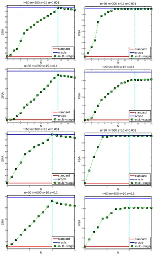
We have performed simulation studies to verify our theoretical analysis. Our comparison includes two aspects: signal recovery accuracy and feature selection accuracy. The signal recovery accuracy is measured by the relative signal error: SRA=₋20 log₁₀(_kβˆ₋β∗_k2/kβ∗k2), where ˆβis the solution of a specific algorithm. The feature selection accuracy is measured by the percentage of correct features selected: FSA=_|_Fˆ_∩_F_|_/_|_F_|_,_{where ˆ}_{F is the estimated feature candidate set.}

We generate an n_×m random matrix X . Each element of X follows an independent

(11)

The s−sparse original signal β∗ is generated with s nonzero elements independently uniformly distributed from [₋10,10]. The locations of s nonzero elements are uniformly distributed in

{1,2,_···,m_}. We form the observation by y=Xβ∗+ε, where the noise vectorε is generated by the Gaussian distribution N(0,σ2_I₎_{. All experiments are repeated 100 times and we use their} average performance for comparison.

First we compare the standard Dantzig selector and the multi-stage version. For a fair compar-ison, we choose the sameλ=σ√2 log m in both algorithms. We run the proposed algorithm with

F₀(0)=∅_{with different values of N and let the estimation ˆ}β _{be the output ˆ}β(N) _{in Algorithm 1.}

The feature candidate set ˆF is predicted by the index set of the s largest elements in ˆβ. Note that ˆF

identified by ˆβ=βˆ(N)_{is different from the output F}(N)

0 by Algorithm 1. The size of ˆF is always

s while the size of F₀(N)is N. Note that the solution of the standard Dantzig selector algorithm is equivalent to ˆβ(N)with N=0. We report the SRA curve of ˆβ(N)with respect to N in the left column of Figure 1. The right column of Figure 1 shows the FSA curve with respect to N. We allow N>s

in our simulation although this case is beyond our theoretical analysis, since in practice the sparsity number s is usually unknown in advance. We can observe from Figure 1 that 1) the multi-stage method obtains a solution with a smaller distance to the original signal than the standard Dantzig selector method; 2) the multi-stage method selects a larger percentage of correct features than the standard Dantzig selector method; 3) the multi-stage method can achieve the oracle solution with a large probability; and 4) even when N>s, the multi-stage algorithm still outperforms the standard

Dantzig selector and achieves high accuracy in signal recovery and feature selection. Overall, the recovery accuracy curve increases with an increasing value of N before reaching the sparsity level s and decreases slowly after that, and the feature selection accuracy curve increases while N≤s and

becomes flat after N goes beyond s.

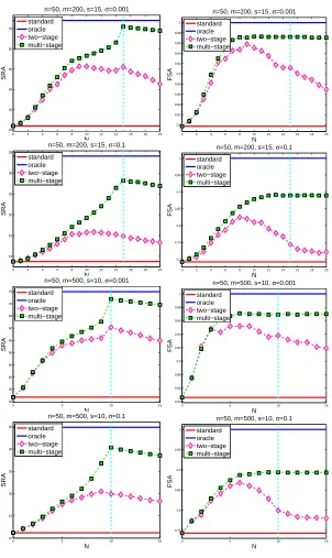
Next we apply the multi-stage procedure to the LASSO case and compare the multi-stage LASSO to the standard LASSO and the two-stage LASSO (Zhang, 2009a). The two-stage LASSO algorithm first estimates a support set F0=suppα(β′)from the solutionβ′ of the standard LASSO whereα>0 is the threshold parameter; the second stage estimates the signal by solving the follow-ing problem

min β :

1

2kXβ−yk 2

2+λ′kβF0¯k1, (8)

which is indeed identical to Equation (7). In order to make it comparable to the proposed multi-stage LASSO algorithm with the parameter N, we properly chooseαsuch that_|F0|=N and use the output ˆβ′from Equation (8) and the feature candidate set by ˆβ′ for comparison. Similarly, we use the sameλ′=2λin the three algorithms. The comparison reported in Figure 2 also indicates the advantage of the proposed multi-stage procedure.

5. Conclusion

(12)

0 2 4 6 8 10 12 14 16 18 20 25 30 35 40 45 50 55 60 65 70 75 N SRA

n=50 m=200 s=15 σ=0.001

standard oracle multi−stage

0 2 4 6 8 10 12 14 16 18 20

0.84 0.86 0.88 0.9 0.92 0.94 0.96 0.98 1 N FSA

n=50 m=200 s=15 σ=0.001

0 2 4 6 8 10 12 14 16 18 20

10 15 20 25 30 35 N SRA

n=50 m=200 s=15 σ=0.1

0 2 4 6 8 10 12 14 16 18 20

0.7 0.75 0.8 0.85 0.9 0.95 1 N FSA

n=50 m=200 s=15 σ=0.1

0 5 10 15

35 40 45 50 55 60 65 70 75 N SRA

n=50 m=500 s=10 σ=0.001

0 5 10 15

0.88 0.9 0.92 0.94 0.96 0.98 1 N FSA

n=50 m=500 s=10 σ=0.001

0 5 10 15

15 20 25 30 35 N SRA

n=50 m=500 s=10 σ=0.1

0 5 10 15

0.75 0.8 0.85 0.9 0.95 1 N FSA

n=50 m=500 s=10 σ=0.1

(13)

0 2 4 6 8 10 12 14 16 18 20 20 30 40 50 60 70 N SRA

n=50, m=200, s=15, σ=0.001 standard

oracle two−stage multi−stage

0 2 4 6 8 10 12 14 16 18 20

0.8 0.82 0.84 0.86 0.88 0.9 0.92 0.94 0.96 0.98 1 N FSA

n=50, m=200, s=15, σ=0.001 standard

0 2 4 6 8 10 12 14 16 18 20

10 15 20 25 30 35 N SRA

n=50, m=200, s=15, σ=0.1 standard

0 2 4 6 8 10 12 14 16 18 20

0.7 0.75 0.8 0.85 0.9 0.95 1 N FSA

n=50, m=200, s=15, σ=0.1 standard

0 5 10 15

30 35 40 45 50 55 60 65 70 75 N SRA

n=50, m=500, s=10, σ=0.001 standard

0 5 10 15

0.84 0.86 0.88 0.9 0.92 0.94 0.96 0.98 1 N FSA

n=50, m=500, s=10, σ=0.001 standard

0 5 10 15

10 15 20 25 30 35 N SRA

n=50, m=500, s=10, σ=0.1 standard

0 5 10 15

0.75 0.8 0.85 0.9 0.95 1 N FSA

n=50, m=500, s=10, σ=0.1 standard

Figure 2: Numerical simulation. We compare the solutions of the standard Dantzig selector method (N =0), the two-stage LASSO algorithm, the proposed method for different values of

(14)

Dantzig selector and the LASSO in both signal recovery and supporting feature selection. The final numerical simulation confirms our theoretical analysis.

Acknowledgments

This work is supported by NSF CCF-0811790, IIS-0953662, and CCF-1025177. We appreciate the constructive comments from the editor and three reviewers.

Appendix A.

Theorem 1 is fundamental for the rest of the theorems. We first highlight a brief architecture for its proof. Theorem 1 estimates_kβˆ₋β∗_kp, which is bounded by the sum of two parts:kβˆ−β∗kp≤ kβˆ−

¯

βkp+kβ¯−β∗kp. We use the upper bounds of these two parts to estimate the bound ofkβˆ−β∗kp.

The analysis in Section 3.2 shows that the first term_kβˆ₋β¯_kp may be much larger than the second

term_kβ¯₋β∗_kp. In Lemma 7, we estimate the bound ofkβ¯−β∗kpand its holding probability. The

remaining part of the proof focuses on the estimation of the bound of_kβˆ₋β¯_kp. For convenience,

we use h to denote ˆβ₋β¯. h can be divided into hF1¯−T1 and hF1+T1, where F0⊂F1⊂F. Lemma 9

studies the relationship between hF1¯−T1 and hF1+T1, if ¯βis feasible (Lemma 8 computes its holding

probability). Then, Lemma 11 shows that_kh_kpcan be bounded in terms ofkhF1+T1kp. In Theorem

12, we estimate the bound of_khF1+T1kp. Finally, letting F1=F, we prove Theorem 1.

Lemma 7 With probability larger than 1₋η(πlog(s/η))−1/2_{, the following holds:}

kβ¯−β∗kp≤

s1/pσp

2 log(s/η)

µ(₍_Xp)T FXF)1/2,s

. (9)

Proof According to the definition of ¯β, we have

¯

βF= (X_FTXF)−1XFTy= (XFTXF)−1XFT(Xβ∗+ε) = (XFTXF)−1XFT(XFβ∗F+ε)

=β∗_F+ (X_FTXF)−1XFTε.

It follows that

¯

(15)

Since kβ¯ −β∗_k_p ₌_k_βF¯ ₋_β∗

Fkp, we only need to consider the bound for kβF¯ −β∗Fkp. Let Z =

(X_FTXF)1/2(β∗F−βF¯ )/σ ∼ N(0,I). We have

P(_kZ_kp≥t) = (2π)−s/2 Z

kZkp≥t

e−ZTZ/2dZ

≤(2π)−s/2

Z

s1/p_k_Z_k ∞≥t

e−ZTZ/2dZ (due to_kZ_kp≤s1/pkZk∞)

=1₋(2π)−s/2Z

kZk∞≤s−1/p_te

−ZTZ/2_dZ

=1−

(2π)−1/2Z

|Zi|≤s−1/pt

e−Zi2/2_dZ

i

s

=1₋

1₋2(2π)−1/2

Z _∞

s−1/p_te

−Z2

i/2_dZ

i

s

≤s

2(2π)−1/2

Z ∞

s−1/p_te

−Z2

i/2_dZ_i

≤ 2s 1+1/p

t(2π)1/2exp

−t2

2s2/p

.

Thus the following bound holds with probability larger than 1−2s1+1/p

t(2π)1/2exp

h

−t2

2s2/p i

:

P(_kZ_kp≤t) =P(k(XFTXF)1/2(β∗F−βF¯ )kp≤tσ)

≤P(µ(₍_Xp)T

FXF)1/2,skβ

∗

F−βF¯ kp≤tσ) =P(kβ∗F−βF¯ kp≤tσ/µ(₍_Xp)T

FXF)1/2,s).

Taking t=p

2 log(s/η)s1/p, we prove the claim. Note that the presented bound holds for any p_≥1.

Lemma 8 With probability larger than 1₋η(πlogm_η−s)−1/2_{, the following bound holds:} kX_FT¯(X ¯β−y)k∞≤λ,

whereλ=σp

2 log(m₋s)/η.

Proof Let us first consider the probability of_kX_FT_¯(X ¯β₋y)_k_∞_≤λ. For any j_∈F, define v¯ jas

vj=XTj (X ¯β−y)

=XT_j XF(XFTXF)−1XFT(XFβ∗F+ε)−XFβ∗F−ε

=XT_j XF(XFTXF)−1XFT−I

ε

∼ _N₍₀_,_XT

j (I−XF(XFTXF)−1XFT)Xjσ2).

Since (I₋XF(XFTXF)−1XFT) is a projection matrix, we have XTj (I−XF(XFTXF)−1XFT)Xjσ2≤σ2.

Thus,

P(_kX_FT¯(X ¯β−y)k∞≥λ) =P(sup

j∈F¯

|vj| ≥λ)≤

2(m₋s)σ

λ(2π)1/2 exp{−λ

(16)

Takingλ=σp

2 log(m−s)/ηin the inequality above, we prove the claim.

It follows from the definition of ¯β that _kX_FT(X ¯β₋y)_k∞=0 always holds. In the following discussion, we assume that the following assumption holds:

Assumption 2 ¯βis a feasible solution of the problem (2), if F0⊂F. Under the assumption above, both_kXT

¯

F(X ¯β−y)k∞≤λandkX T

F(X ¯β−y)k∞=0 hold.

Note that this assumption is just used to simplify the description for following proofs. Our proof for the final theorems will substitute this assumption by the probability it holds.

In the following, we introduce an additional set F1satisfying F0⊂F1(Zhang, 2009a).

Lemma 9 Let F0⊂F. Assume that Assumption 2 holds. Given any index set F1such that F0⊂F1,

we have the following conclusions:

kh_F0¯₋_F1¯k1+2kβ¯_F1¯k1≥kh_F1¯k1 kX_F0TX hk∞=0

kX_FT¯X hk∞≤2λ kXF0T¯−F¯X hk∞≤λ.

Proof Since ¯βis a feasible solution, the following holds

kβˆF0¯k1≤ kβ¯F0¯k1

kβˆF0¯−F1¯k1+kβˆF1¯k1≤ kβ¯F0¯−F1¯k1+kβ¯F1¯k1 kβˆ_F1¯k1≤ kh_F0¯₋_F1¯k1+kβ¯_F1¯k1 kh_F1¯ +β¯_F1¯k1≤ kh_F0¯₋F1¯k1+kβ¯_F1¯k1

khF1¯k1≤ khF0¯−F1¯k1+2kβ¯F1¯k1. Thus, the first inequality holds. Since

X_F0TX h=X_F0TX(βˆ₋β¯) =X_F0T(X ˆβ₋y)₋X_F0T(X ¯β₋y),

the second inequality can be obtained as follows:

kX_F0TX h_k∞≤ kX_F0T(X ˆβ₋y)_k∞+_kX_F0T(X ¯β₋y)_k∞=0.

The third inequality holds since

kX_FT_¯X h_k_∞_{≤ k}X_FT_¯(X ˆβ₋y)_k_∞+_kX_FT_¯(X ¯β₋y)_k_∞_≤2λ.

Similarly, the fourth inequality can be obtained as follows:

kXF0T¯₋F¯X hk∞≤ kX

T

¯

F0₋F¯(X ˆβ−y)k∞+kX

T

¯

(17)

Lemma 10 Given any v∈Rm_{, its index set T is divided into a group of subsets T}_j_{’s ( j}₌₁_,₂_{, ...}₎

without intersection such thatS_jTj=T . If maxj|Tj| ≤l and maxi_∈Tj+1|vTj+1[i]| ≤ kvTjk1/l hold for

all j’s, then we have

kvT1¯kp≤ kvk1l1/p−1.

Proof Since_|vTj+1[i]| ≤ kvTjk1/l, we have kvTj+1k

p

p=

∑

i∈Tj+1

|v_Tp_j₊₁[i]_{| ≤ k}vTjk

p

1l 1−p_,

⇒ kvTj+1kp≤kvTjk1l 1/p₋1_. Thus,

kv_T1¯kp≤

∑

j≥1

kvTj+1kp≤

∑

j≥1

kvTjk1l

1/p−1₌

kv_k1l1/p−1, which proves the claim.

Note that similar techniques as those in Lemma 10 have been used in the literature (Cand`es and Tao, 2007; Zhang, 2009a).

Lemma 11 Assume that F0⊂F and F0⊂F1. We divide the index set ¯F1into a group of subsets Tj’s

( j=1,2, ...) such that they satisfy all conditions in Lemma 10 with v=h. Then the following holds:

khF1¯−T1kp≤l

1/p−1_|_F_¯

0−F¯1|1−1/pkhF0¯−F1¯kp+2kβ¯F1¯k1

,

kh_kp≤

"

1+

|_F¯₀₋_F¯₁_|

l

p−1#1/p

khF1+T1kp+2l1/p−1kβ¯_F1¯k1.

Proof Using Lemma 10 with T =_F¯₁_{, the first inequality can be obtained using the first inequality} in lemma 9 as follows:

kh_F1¯₋_T1kp≤l1/p−1kh_F1¯k1≤l1/p−1 kh_F0¯₋_F1¯k1+2kβ¯_F1¯k1

≤l1/p−1

|_F¯₀₋_F¯₁_|1−1/p_k_h

¯

F0₋F1¯kp+2kβ¯F1¯k1

.

For any x_≥0, y_≥0, p_≥1, and a_≥0, it can be easily verified that

(xp+ (ax+y)p₎1/p_≤₍₁₊_ap₎1/p_x₊_y_. ₍₁₀₎

It follows that

kh_kp=

khF1+T1k p

p+khF1¯₋T1kpp

1/p ≤

"

khF1+T1kpp+

"

|_F¯₀₋_F¯₁_|

l

1−1/p

khF0¯₋F1¯ kp+2l1/p−1kβ¯F1¯k1 #p#1/p

≤ "

1+

|_F¯₀₋_F¯₁_|

l

p−1#1/p

khF1+T1kp+2l

(18)

The first inequality is due to the first claim in this lemma; the second inequality is due tokhF0¯₋F1¯kp≤

khF1+T1kpand (10). We complete the proof for the second claim.

Theorem 12 Under Assumption 1, taking F0⊂F and λ=σ r

2 log

m−s

η1

into the optimization

problem (2), for any given index set F1 satisfying F0 ⊂F1 ⊂F , if there exists some l such that

µ(_Ap_,_s1)₊_l₋θ(_Ap_,_s1)₊_l_,_l

|F0¯−F1¯|

l

1−1/p

>0 holds where s1=|F1|, then with probability larger than 1−η′1,

theℓp norm (1≤p≤∞) of the difference between the optimizer of the problem (2) and the oracle

solution is bounded as

kβˆ−β¯kp≤

1+|F0¯−_lF1¯|p−1 1/p

(_|_F¯₀₋_F¯₁_|₊₂p_l₎1/p_λ₊₂_θ(p)

A,s1+l,ll1/p−1kβ¯F1¯k1

µ(_Ap_,_s1)₊_l₋θ(_Ap_,)_s1₊_l_,_l

|F0¯−F1¯|

l

1−1/p +2l1/p−1kβ¯F1¯k1

and with probability larger than 1₋η′₁₋η′₂, the ℓpnorm (1≤p≤∞) of the difference between the

optimizer of the problem (2) and the true solution is bounded as

kβˆ−β∗kp≤

1+|F0¯−_lF1¯|p−1 1/p

(_|_F¯₀₋_F¯₁_|₊₂p_l₎1/p_λ₊₂_θ(p)

µ(_Ap_,)_s1₊_l₋θ(_Ap_,_s1)₊_l_,_l

|F0¯−F1¯|

l

1−1/p

+2l1/p−1_kβ¯_F1¯k1+

s1/p µ(₍_Xp)T

FXF)1/2,s

σp

2 log(s/η2).

Proof First, we assume Assumption 2 and the inequality (9) hold. Divide ¯F1into a group of subsets

Tj’s ( j=1,2, ...) without intersection such that SjTj =F¯1, maxj|Tj| ≤l and maxi∈Tj+1hTj+1[i]≤

khTjk1/l hold. Note that such a partition always exists. Simply, let T1be the index set of the largest

(19)

conditions above. For convenience of presentation, we denote T0=F¯0−F¯1and T01=T0+T1. Since kX_TT₀₁₊_F0X h_kp

=_kX_TT₀₁₊_F0XT01+F0hT01+F0+

∑

j≥2

X_T01T ₊_F0XTjhTjkp

≥µ(_Ap_,)_s1₊_l_khT01+F0kp−

∑

j≥2

θ(p)

A,s1+l,lkhTjkp

≥µ(_Ap_,)_s1₊_l_khT01+F0kp−θ(_Ap_,_s1)₊_l_,_l

∑

j≥2

khTjkp

≥µ(_Ap_,)_s1₊_l_khT01+F0kp−θ_A(p_,_s1)₊_l_,_ll1/p−1kh_F1¯k1 (due to lemma 10) ≥µ(_Ap_,)_s1₊_l_khT01+F0kp−θ(

p)

A,s1+l,ll

1/p₋1

khT0k1+2kβ¯F1¯k1

(due to lemma 9)

≥µ(_Ap_,)_s1₊_lkhT01+F0kp−θ(_Ap_,_s1)₊_l_,_l

l

|T0| 1/p−1

khT0kp−2θ(_Ap_,_s1)₊_l_,_ll1/p−1kβ¯F1¯k1

≥ µ(_Ap_,_s1)₊_l₋θ(_Ap_,)_s1₊_l_,_l

l

|T0|

1/p−1!

khT01+F0kp−2θ(_Ap_,_s1)₊_l_,_ll1/p−1kβ¯F1¯k1

and

kX_T01T ₊_F0X h_kp_p

=_kX_F0TX h_kp_p+_kX_TT₀₁_∩_FX h_kp_p+_kX_TT

01∩F¯X hk p p

≤|T01∩F|λp+|T01∩F¯|(2λ)p (due to lemma 9)

≤|T0∩F|λp+|T1∩F|λp+|T0∩F¯|(2λ)p+|T1∩F¯|(2λ)p (due to F1⊂F) ≤|T0|λp+l(2λ)p, (due to T0∩F¯=∅)

we have

khF1+T1kp=khT01+F0kp≤

(_|T0|+2pl)1/pλ+2θ(

p)

µ(_Ap_,_s1)₊_l₋θ(_Ap_,_s1)₊_l_,_l

l

|T0|

1/p−1

=(|

¯

F0−F¯1|+2pl)1/pλ+2θ(_Ap_,_s1)₊_l_,_ll1/p−1kβ¯F1¯k1

µ(_Ap_,_s1)₊_l₋θ(_Ap_,_s1)₊_l_,_l

|_F0¯₋_F1¯_|

l

1−1/p .

Due to the second inequality in Lemma 11, we have

kh_kp≤

"

1+

|_F¯₀₋_F¯₁_|

l

p−1#1/p

khF1+T1kp+2l

1/p−1_k_β_¯ ¯

F1k1

=

1+|F0¯−_lF1¯|p−1 1/p

(_|_F¯₀₋_F¯₁_|₊₂p_l₎1/pλ₊₂θ(p)

µ(_Ap_,_s1)₊_l₋θ(_Ap_,_s1)₊_l_,_l

|F0¯−F1¯|

l

1−1/p +

(20)

Thus, we can boundkβˆ−β∗_k_p_as

kβˆ−β∗kp≤kβˆ−β¯kp+kβ¯−β∗kp

≤

1+|F0¯−_lF1¯|p−1 1/p

(_|_F¯₀₋_F¯₁_|₊₂p_l₎1/p_λ₊₂_θ(p)

A,s1+l,ll

1/p₋1_k_β_¯ ¯

F1k1

µ(_Ap_,)_s1₊_l₋θ(_Ap_,_s1)₊_l_,_l

|_F0¯₋_F1¯_|

l

1−1/p

+2l1/p−1_kβ¯F1¯k1+

s1/p µ(₍_Xp)T

FXF)1/2,s

σp

2 log(s/η2).

Finally, takingλ=σ r

2 log

m₋s

η1

, Lemma 8 withη=η1 implies that Assumption 2 holds with probability larger than 1₋η′₁ and Lemma 7 withη=η2 implies that (9) holds with probability larger than 1₋η′₂. Thus, these two bounds above hold with probabilities larger than 1₋η′₁ and 1₋η′₁₋η′₂, respectively.

Remark 13 Cand`es and Tao (2007) provided a more general upper bound for the Dantzig

selec-tor solution in the order of

O

k1/2σ√_{log m}₊_r(2)

k (β∗)

√

log m, where 1_≤k_≤s and r(_kp)(β) =

∑i_∈Lk|βi|

p1/p

(Lk is the index set of the k largest entries in β). We argue that the result in

Theorem 12 potentially implies a tighter bound for Dantzig selector. Setting F0 =∅

(equiva-lent to the standard Dantzig selector) and l =k with k=_|_F¯₁_|_{in Theorem 12, it is easy to verify}

that the order of the bound for _kβDˆ ₋β¯_kp is determined by

O

k1/pσ√log m+k1/p−1r(1)_k (β¯), or

O

k1/pσ√log m+k1/p−1r(1)_k (β∗)due to Lemma 7. This bound achieves the same order as the bound of the LASSO solution given by Zhang (2009a), which is the sharpest bound for LASSO to our knowledge.

We are now ready to prove Theorem 1.

Proof of Theorem 1: Taking F1=F in theorem 12 which indicates that ¯βF1¯ =0, we conclude that

kβˆ−β¯kp≤

1+|F0¯−_lF¯|p−1 1/p

(_|_F¯₀₋_F¯_|₊_l2p₎1/p

µ(_Ap_,_s)₊_l₋θ(_Ap_,_s)₊_l_,_l

|_F0¯₋_F¯_|

l

1−1/p λ

holds with probability larger than 1₋η′₁and

kβˆ−β∗kp≤kβˆ−β¯kp+kβ¯−β∗kp

≤

1+|F0¯−_lF¯|p−1 1/p

(_|_F¯₀₋_F¯_|₊_l2p₎1/p

µ(_Ap_,_s)₊_l₋θ(_Ap_,_s)₊_l_,_l

|_F0¯₋_F¯_|

l

1−1/p λ+

s1/p µ(p)

(XT FXF)1/2,s

σp