An Information Criterion for Variable Selection
in Support Vector Machines
Gerda Claeskens [email protected]
Christophe Croux [email protected]
Johan Van Kerckhoven [email protected]
ORSTAT and Leuven Statistics Research Center Katholieke Universiteit Leuven
B-3000 Leuven, Belgium
Editors: Isabelle Guyon and Amir Saffari
Abstract
Support vector machines for classification have the advantage that the curse of dimensionality is circumvented. It has been shown that a reduction of the dimension of the input space leads to even better results. For this purpose, we propose two information criteria which can be computed directly from the definition of the support vector machine. We assess the predictive performance of the models selected by our new criteria and compare them to existing variable selection techniques in a simulation study. The simulation results show that the new criteria are competitive in terms of generalization error rate while being much easier to compute. We arrive at the same findings for comparison on some real-world benchmark data sets.
Keywords: information criterion, supervised classification, support vector machine, variable
se-lection
1. Introduction
We study classification using the support vector machine (SVM). We start from a training set {(xi,yi)}containing n observations. Each p-dimensional observation xi= (xi1, . . . ,xip)has a class label yi assigned to it, which is either+1 or−1. We wish to find a function f(·) such that for an observation x the predicted class ˆy= +1 if f(x)is positive, and ˆy=−1 if f(x)is negative. We want this function to assign the correct class labels to the training observations (low training error rate) and to accurately classify new observations (low generalization error rate). Working with a subset of the p variables xi1, . . . ,xipreduces variability of the class-label estimator and might lead to better out-of-sample predictions.
generalization properties (high generalization error rate) cannot be avoided. Guyon et al. (2002) illustrate this and show that variable selection can further improve the SVM’s performance.
Variable selection techniques can be divided into three categories. Filters select subsets of vari-ables as a pre-processing step, independently of the prediction method. Wrappers use the classifica-tion method to score subsets of variables. Finally, embedded methods include variable selecclassifica-tion into the construction of the classifier. In this paper we propose new information criteria for SVMs, yield-ing a wrapper method where we consider the SVM merely as a black box. We refer to Guyon and Elisseeff (2003) for an introduction to variable and feature selection in Machine Learning. Informa-tion criteria are a standard tool for model selecInforma-tion in tradiInforma-tional statistics. InformaInforma-tion criteria for variable selection assign a numerical value to each subset of the variables under consideration. The subset with the lowest value of the information criterion is then selected. Examples are the Akaike information criterion (AIC, Akaike, 1973) and the Bayesian information criterion (BIC, Schwarz, 1978). Claeskens and Hjort (2008) survey and explain the use of common information criteria for statistical variable selection in likelihood-based models, we refer to there for more references.
For support vector machines only very few information criteria have been developed. The kernel regularisation information criterion (KRIC) of Kobayashi and Komaki (2006) was originally pro-posed for parameter tuning of the SVM. We apply it for variable selection. However, the KRIC has a complicated definition and is computationally expensive for large sample sizes. In this paper two new information criteria are proposed, one shares properties with AIC, the other with BIC. We want the new criteria to select a preferably compact subset of variables with good predictive properties. We will show that submodels selected by the new criteria are as performing as the ones chosen by the KRIC, while they incur substantially less computational overhead. We also make a comparison with using cross-validated error rate based criteria, as in Kearns et al. (1997). An important contri-bution of this paper is that our numerical comparisons show that the popular, but time consuming, cross-validation criteria are outperformed in generalization error by the new information criteria, where the latter are coming at almost no additional computational cost.
Alternative approaches perform variable selection in feature space instead of in input space (Shih and Cheng, 2005), or select a set of “maximally separating directions” in the input space (Fortuna and Capson, 2004). These methods, however, do not select a set of original input variables. Various other authors have suggested different formulations for the SVM such that variable selection is performed automatically. Examples of such embedded methods can be found in Bi et al. (2003), Zhu et al. (2004), Neumann et al. (2005), Lee et al. (2006), Wang et al. (2006), Zhang (2006), and Lin and Zhang (2006).
In Section 2 we define the support vector machine setting, we review existing information cri-teria and we describe ranking techniques to speed up the variable selection process. In Section 3, we define the new information criteria and highlight their advantages. Section 4 contains the results of a simulation study and in Section 5 we compare the different techniques on a few real-world benchmark data sets. Section 6 concludes and gives some directions for further research.
2. Problem Setting
2.1 The Support Vector Machine
We denote the training sample (xi,yi), 1≤i≤n, with xi a p-dimensional vector of explicative variables, and yi ∈ {−1,+1}the class label. The goal is to estimate a target function f(x) in the space of explicative variables such that f(xi)>0 for yi= +1, and f(xi)<0 for yi=−1.
We start with linear support vector machines, where f(x) is of the form f(x) =w0x+b.For binary classification this function is obtained by solving the minimisation problem
min w,b,ξi
(
1 2kwk
2+C
∑
n i=1ξi
)
subject to
(
yi(w0xi+b)≥1−ξi,
ξi≥0,i=1, . . . ,n.
(1)
The ξi are slack margin variables, indicating how close a point xi lies to the separating boundary
(ifξi<1), or how badly it is misclassified (ifξi>1). The tuning parameter C controls how much weight is put on trying to achieve perfect separation.
The dual problem can be solved more easily, and has the following form:
min
α {
1 2α
0Qα−
∑
ni=1
αi}subject to
0≤αi≤C, i=1, . . . ,n,
∑n
i=1yiαi=0. (2) Hereαi is the weight given to the observation(xi,yi), and Q is a positive semi-definite matrix with entries Qi,j=yiyjxi0xj. The vector w can be found from w=∑ni=1yiαixi.The negative intercept b is found by computing b=0.5(r2−r1), where
r1=
∑0<yiαi<C(Qα)i−1
∑0<yiαi<C1
and r2=∑0>yiαi>−C(Qα)i−1
∑0>yiαi>−C1
.
If no i exist for which 0<yiαi<C, then define
r1= 1 2
min
αi=0,yi=1
(Qα)i− max
αi=C,yi=1
(Qα)i
,
and analogously for r2, with yi =−1. Note that we can write ξi = [1−yiai]+, where [x]+ =
max{0,x}and where ai= f(xi).
The linear SVM can be extended towards more complex decision functions in a rather straight-forward way. Therefore we replace the inner products x0ixjin the definition of Q by a more general kernel function K(xi,xj). See Cristianini and Shawe-Taylor (2000) for the properties that these kernel functions must have. This leads to a more general decision function
f(x) = n
∑
i=1
yiαiK(xi,x) +b. (3)
Popular choices for the kernel function in (3) are the linear kernel, where the kernel function is K(x,z) =x0z, the polynomial kernel of the form K(x,z) = (c0+γx0z)d, and the radial basis kernel K(x,z) =exp(−γkx−zk2), where c0, γand d are regularization parameters that can be tuned for optimal performance of the classifier. In this more general setting, we have
kwk2= n
∑
i,j=1
yiyjαiαjK(xi,xj) =α0Qα
2.2 Existing Variable Selection Techniques for SVM
We compare our new methods (Section 3) to variable selection based on (ten-fold) cross-validation (CV), guaranteed risk minimisation (GRM, Vapnik, 1982) and the kernel regularisation information criterion (KRIC) by Kobayashi and Komaki (2006). Each of these will be explained in more detail below.
Ten-fold cross-validation divides the training data in ten parts of roughly equal size. One part is left out, the other nine parts are the training data and are used to fit the SVM. This SVM is applied to the part that is left out to obtain an estimate of the error rate. This process is repeated ten times (each time a different part is left out) to obtain the CV generalization error rate ˆε(S)as the average of the ten separate error rates. We select the model with the lowest value of ˆε(S), where S ranges over all subsets of variables under consideration. Another common method is five-fold CV. The lower the number of folds, the less computing time is required, but the higher the variability of
the estimates of the generalization error. Note that n−fold CV is the same as the computationally
infeasible leave-one-out CV.
General risk minimisation (Vapnik, 1982) is derived from the estimated generalization error rate, using
GRM(S) =εˆ(S) +|S|
n 1+
p
1+εˆ(S)(n/|S|)
. (4)
Here,|S|stands for the number of input variables in the set S and n is the number of observations
in the training sample. We select the model with the lowest value of GRM(S), where S ranges over
all subsets of variables under consideration. Kearns et al. (1997) compare CV, GRM and mini-mum description length (Rissanen, 1989). Their experiments have demonstrated that none of the criteria is consistently better than the others. Note that the computational overhead for computing these measures can be immense, since we need to train ten support vector machines to estimate the generalization error rate for only one submodel.
We now define the KRIC of Kobayashi and Komaki (2006). This criterion was originally de-veloped to tune the constant C in the SVM definition (1), and by extension to tune the kernel
pa-rameters. We use it without much adjustment for variable selection. Denote by xi,Sthe subvector of
xi, consisting of elements xi j with j∈S, and similarly for other vectors. We estimate the SVM (1) using the observations(xi,S,yi), yielding the vectorsωS,bS andξS, where the subscript S refers to the subset of variables under consideration. In the dual problem (2), we haveαS= (αS,1, . . . ,αS,n) and[QS]i,k=yiykK(xi,S,xk,S). The decision rule fS(x)is as in (3), and we set ai,S= fS(xi,S).Next,
we define vectors tSand mSof length n, with components
tS,i=η2
exp(−ηai,Syi) (1+exp(−ηai,Syi))2
and mS,i=−η
yiexp(−ηai,Syi) 1+exp(−ηai,Syi)
, i=1, . . . ,n.
Here we choose η=log(2) such that log(1+exp(−ηx)) and η[1−x]+ coincide for x=0, see
Kobayashi and Komaki (2006) for further motivation. Withλ=C−1log 2 the KRIC for the logistic
Bayesian model for SVMs is defined as
KRIC(S) = 2
n
∑
i=1
log 1+exp(−ηai,Syi)
(5)
+trace((QSdiag(tS) +λIn)−1QS(diag(mS)2−n−1mSmtS))
Alternatively, Sollich’s Bayesian model for SVMs (Sollich, 2002) leads to a KRIC with a similar form as the one in (5). Using
ν(ai,S) = (1+exp(−2C))−1(exp(−C[1−ai,S]+) +exp(−C[1+ai,S]+)),
the KRIC for the Sollich Bayesian model for SVMs is defined as
KRICS(S) =KRIC(S)−2n log n
∑
i=1
ν(ai,S). (6)
The computation of the KRIC includes inverting an n×n-matrix with only a few zeroes. Therefore,
the computation is time-consuming if the sample size n is large. Both the CV error rate and the KRIC may require a prohibitive computing time when a large number of different models needs to be evaluated.
2.3 Ranking Techniques
A full subset search is computationally not feasible even not for problems with only a small number
of dimensions (p=15 for example). To dramatically reduce the number of models while still
selecting a model that is “almost” the best model, Chen et al. (2005) use a genetic algorithm, while Peng et al. (2005) suggest a combined backward elimination/forward selection strategy. However, both of these techniques still suffer from the possibility that a large number of models needs to be checked before arriving at a solution.
Alternatively, variable ranking consists of assigning a “value of importance” to each variable and sorting the variables according to their importance. This results in a series of p stacked models, thus only p evaluations of the variable selection criterion are needed. The most commonly used algorithm is the SVM recursive feature elimination (SVM-RFE) technique from Guyon et al. (2002).
For a linear SVM, the variables are ranked by w2j, with wjthe j-th component of the weight vector
w. This technique assumes that the variables are standardized to have mean 0 and variance 1. The extension proposed by Rakotomamonjy (2003) allows application to SVMs with a non-linear kernel. We use the following SVM-RFE algorithm with variable influence
∆kwSk2(j)=
kwSk2− kwS\{j}k2
as suggested by Rakotomamonjy (2003).
Step 1: Initialise S← {1, . . . ,p}, the subset of unranked features, and r←(), the vector of ranked features.
Step 2: Repeat the following steps until S= /0.
(a) Train a SVM on(xi,S,yi), and computekwSk2=α0SQSαS.
(b) For each j∈ S, train a new SVM on (xi,S\{j},yi). This gives a value kwS\{j}k2 =
α0
S\{j}QS\{j}αS\{j}for each j∈S.
The vector r contains the ranked variables, with the first element the most important one. A
disad-vantage of this method is that the number of SVMs to be trained is
O
(p2). This can be overcome byusingαSinstead ofαS\{j}in Step 2b, such thatkwS\{j}k2≈α0SQS\{j}αS. Rakotomamonjy (2003) argues that this will not affect the ranking significantly, while still allowing a major reduction in
computational time, bringing the number of SVMs to be estimated to
O
(p). We employ thisap-proximation in the simulation study in Section 4 and in the real data examples in Section 5.
The most easy way to rank the variables is by filtering methods. Zhang et al. (2006) propose using sj =|wj(mj,+1−mj,−1)|for ranking, where mj,+1 and mj,−1 are the within-class means of variable j. Shih and Cheng (2005) use the Fisher score
Sj= |
mj,+1−mj,−1|
q
σ2
j,+1+σ2j,−1
for a linear SVM, where σ2j,+1 andσ2j,−1 are the within-class variances of variable j. The main
advantage of using Sj is that it is not necessary to train any SVM to rank the variables. The Fisher
score ranking is considered in Sections 4 and 5.
3. The New Information Criteria
As stated in the previous section, evaluating the CV error rate or the KRIC of a particular sup-port vector machine model requires a high number of additional computations. For this reason, we propose two new criteria which use information already available in the SVM, without additional complicated computations. The criteria are based on how badly the SVM violates the margin con-straints, which are written as∑ni=1ξi,S,whereξi,Sis the margin slack of observation i in the support vector machine trained on the variables with indices in S, where S is a subset of{1, . . . ,p}. Alter-natively, we can use the logarithm of this sum, analogous to Bai and Ng (2002) for selecting the number of factors in factor analysis. However, in the SVM setting this has the drawback that the value is undefined if the sum equals zero, which can happen if the data are perfectly separable. Also, Bai and Ng (2002) advise using a log-transform for scalar invariance reasons. Since we follow the advice to standardise the variables before training the SVM, for better ranking as explained in Sec-tion 2.3, we automatically have scalar invariance of the sum of the margin slacks. For these reasons, we choose not to take the log-transform.
Generally (but not always),∑iξi,Swill decrease as more variables are added. Therefore we add a penalty term related to the number of included variables to ensure a tradeoff between accuracy and simplicity of the chosen model. We suggest adding a linear penalty term, such that we get an information criterion of the form
IC(S) = n
∑
i=1
ξi+C(n)|S|, (7)
where S is the set of variables included in the model.
A first choice is to take C(n) constant in (7). It is interesting to note that IC(S) is then, up to constant factors, an easily computable approximation of the KRIC of Kobayashi and Ko-maki (2006), hereby providing a theoretical justification for its use. To better understand this, note first that log 1+exp(−ηai,Syi)
η[1−yiai,S]+=ηξi,Sfor all 1≤i≤n. Hence, the first term of the KRIC can be approximated, up to a constant factor, by∑iξi,S. For the approximation of the second term in (5), rewrite
W = (QSdiag(tS) +λIn)−1QS(diag(mS)2−n−1mSmtS) = V diag(tS)−1(diag(mS)2−n−1mSmtS),
with V = (A+λIn)−1A a symmetric, positive semi-definite matrix and A=QSdiag(tS). Denoting
A− the generalised inverse of A, and using a series expansion aroundλ=0, gives that the leading
term of V=A−(I+λA−)−1A is equal to A−A. This expansion converges as long as the eigenvalues
ofλA− are strictly less than one, which can be obtained by taking λsmall enough. We now use
a singular value decomposition of both A and A− and use the fact that the singular values of A−
are the reciprocals of the non-zero singular values of A, to obtain that the product A−A is a n×n
diagonal matrix with on the diagonal|S|ones and the remaining entries zero. Thus, the leading term
of trace(W)equals the sum of|S|diagonal entries of the matrix diag(tS)−1(diag(mS)2−n−1mSmtS)). The i-th diagonal element of this matrix is equal to
n−1 n t
−1 S,im2S,i=
n−1
n exp(−ηai,Syi).
To further facilitate computations we replace this by 1, motivated by the fact thatηai,Syi is often small. Although this approximation might be crude for a single term, we found empirically that it works well for the summation over the entire training set. Hence, we arrive at the approximation trace(W)≈ |S|which is the linear penalty term in (7).
Taking the constant value C(n) =2, leads to our first new support vector machine information
criterion (SVMIC):
SVMICa(S) =
n
∑
i=1
ξi+2|S|. (8)
The newly proposed criterion SVMICa for support vector machines shares the form of the penalty with the well-known Akaike (1973) information criterion. This AIC is defined as minus twice the value of the maximised log likelihood of the model, plus two times the number of parameters to be estimated (that is, 2|S|). Because the penalty 2|S| is not dependent on the sample size n, we expect that both criteria share some properties, such as having the tendency to not select the most
parsimonious model. For the AIC, Woodroofe (1982) has shown that in the limit for n→∞, the
expected number of superfluous parameters is less than one.
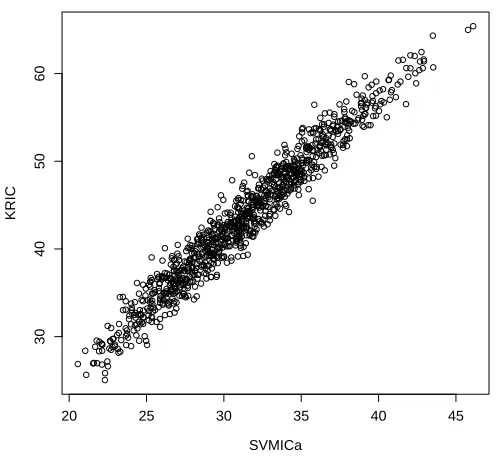
To support the definition of SVMICa , we ran a simulation experiment and compared the values
of KRIC and SVMICa for 100 models. The sample size is n=50, with 10 variables of which only
the first 4 variables are different from zero. A detailed description of the simulation setting can be found in Section 4. We used a linear kernel. Figure 1 reports these numerical results and shows a high correlation (0.975) between the values of the two criteria. Other simulation settings gave comparable correlation values.
Our second proposed criterion follows the spirit of Bayesian information criterion (BIC) by Schwarz (1978). This criterion is defined similarly as the AIC, but instead of the penalty 2|S|, it
uses log(n)|S|. The BIC has been shown to be consistent (Haughton, 1988, 1989). This means that
20 25 30 35 40 45
30
40
50
60
SVMICa
KRIC
Figure 1: Values of KRIC and SVMICa in a simulation experiment, showing high correlation (0.975).
us to take C(n) =log(n), and we define our second criterion
SVMICb(S) =
n
∑
i=1
ξi+log(n)|S|. (9)
It is immediate that the computational cost of both SVMICs is much lower than of the cross-validated error rate (10 more SVMs to train for 10-fold cross-validation) and of the kernel
regulari-sation information criterion KRIC (which needs computations of the order
O
(n3)due to the matrixinversion). The best case is when theξi,Sare directly available. Computing the SVMICs is only an
O
(n)computation in that case, and usually even less when employing the property thatξi,S6=0⇔αi,S=1.
When onlyαSand QSare available,ξi,Sis computed using the relation
ξi,S=
h
1−yi n
∑
j=1
αj,S>0
αj,S[QS]i j
i
+.
4. Simulation Results
We perform M=100 simulation runs with the following settings. We generate n∈ {25,50,100,200}
independent observations xi, 1≤i ≤n of dimension p ∈ {25,50,100,200}, with distribution
N
(0,σ2Ip) where σ2=1. For each observation we generate a class label yi ∈ {−1,+1}, with
P(yi =1) =1/2. Finally, we let µ = (1/2,−1/2,−1/2,1/2,0, . . .,0) of dimension p, and set xi ←xi+yiµ to separate the two classes to some extent. This implies that the optimal separat-ing hyperplane is x0µ=0, such that ˆy= +1 if x0µ>0, resulting in a generalization error rate of
Φ(−kµk2/σ), withΦ the cumulative distribution function of a standard normal. In our example,
withσ=1 andkµk2=1, we find an optimal generalization error rate of 0.159.
During each simulation run, we standardize the variables to improve the numerical performance of the SVM algorithm. The variables are ranked using either the Fisher score or based on the variable influence on w, as described in Section 2.3. For each of the nested models obtained in the variable ranking step, we compute (i) SVMICa and (ii) SVMICb as in (8) and (9). We compare their performance to (iii) ten-fold CV, (iv) Vapnik’s GRM as in (4), (v) KRIC for the logistic Bayesian model for SVMs as in (5), and (vi) KRIC for the Sollich model for SVMs as in (6). An important remark is that for ten-fold CV, we employ the CV2 method, which includes the feature selection procedure in each cross-validation step, as suggested by Zhang et al. (2006). Computing the CV error rate in the usual way can lead to a (severely) biased estimate of the generalization error, and using CV2 reduces this bias.
The experiment is repeated with two different kernels (i) a linear kernel K(x1,x2) =x01x2leading to a linear decision rule (ii) a quadratic kernel K(x1,x2) = (γx01x2+1)2, withγ=1/p, the inverse of the number of variables, leading to a quadratic decision rule. The tuning parameter C in each
SVM that we train is chosen to be C=1, as we standardize the explicative variables a priori. This
is also the standard setting for C for thesvmprocedure in theRsoftware package. We experimented
with other values of C in the range from 0.1 up to 10, and found only minor differences in the simulation outcomes. We test the accuracy of the classifiers computed from the selected input variables by estimating their generalization (out-of-sample) error rate from a test sample of 10000 new observations. These observations are generated in the same way as the training sample.
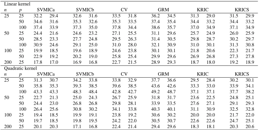
Table 1 reports the generalization error rates, obtained by averaging over the 100 simulation runs. An overall observation is that the error-rate based selection criteria (CV and GRM) have the worst performance. The performances of the KRICs and the new SVMICs are comparable. More precisely, we observe that the KRICs are better as a variable selection method for small sample sizes
(n=25), while the SVMICs give better results for larger sample sizes. This is especially apparent
when the quadratic kernel is used. For a small number of observations compared to the number of variables, we also note that SVMICa slightly outperforms SVMICb in terms of generalization error rate, and that the opposite is true with many observations and fewer variables. The differences in generalization error rates become smaller as the number of variables grows. This is particularly true for CV, whose relative performance becomes better at large sample sizes. But SVMICa and SVMICb are still somewhat ahead, and have the advantage that they are much easier (and less time-intensive) to compute than the other criteria, included the KRICs having a computation time
of order
O
(n3). Note that, as n grows, the generalization error rates of the models obtained byLinear kernel
n p SVMICa SVMICb CV GRM KRIC KRICS
25 25 32.2 29.4 32.6 31.6 33.5 31.8 36.2 34.5 31.3 29.0 31.5 29.9 50 34.6 31.6 35.3 32.6 35.3 33.5 37.4 35.4 34.4 33.2 34.4 33.2 100 37.4 33.9 37.3 35.0 37.8 34.4 38.6 35.7 37.0 34.9 37.1 34.9 50 25 24.4 21.6 24.6 23.2 27.1 25.5 31.1 29.6 25.7 24.9 26.0 25.9 50 28.5 23.3 27.7 24.8 29.5 26.3 31.4 30.5 29.8 28.7 30.2 29.7 100 30.9 24.6 29.1 25.0 31.0 28.0 32.1 30.9 31.0 30.1 31.3 30.8 100 25 19.9 18.5 19.6 18.9 24.6 23.8 30.1 30.1 21.8 20.6 22.3 21.7 50 22.9 19.2 20.2 19.0 25.8 25.4 29.9 29.6 26.9 26.8 27.3 27.8 200 25 17.8 17.0 16.9 16.8 22.7 21.5 28.9 29.3 18.7 18.0 19.2 18.9 Quadratic kernel
n p SVMICa SVMICb CV GRM KRIC KRICS
25 25 31.3 30.7 34.2 33.8 33.8 32.9 37.7 36.6 29.5 28.4 30.2 30.1 50 35.8 35.3 39.3 38.5 39.6 38.5 43.6 42.6 33.3 33.0 33.9 34.1 100 43.3 43.3 48.3 48.4 42.8 42.7 49.2 48.7 37.1 37.1 37.7 38.2 50 25 22.7 21.3 25.0 24.3 26.7 25.9 31.8 31.7 23.6 22.5 24.8 25.1 50 24.4 23.0 26.8 26.8 29.8 28.1 33.9 33.5 27.6 27.1 29.1 29.3 100 26.4 25.6 30.8 30.2 34.1 33.8 40.3 40.1 31.1 30.9 32.5 32.8 100 25 19.4 18.5 19.9 19.1 23.8 19.2 30.6 30.2 20.0 20.0 21.7 22.0 50 19.7 18.5 19.8 19.5 24.2 22.0 30.5 30.7 22.6 22.6 24.7 25.1 200 25 20.1 20.3 17.1 16.8 22.4 21.4 29.4 29.6 18.3 18.1 20.3 20.6
Table 1: Simulated average generalization error rate (%) for the six methods using two different kernels. For each method, the number on the left resulted from ranking by variable
influ-ence onkwk2, and the number on the right in each column is from ranking by the Fisher
scores Sj.
kernels to a strong preference for ranking with the Fisher score. For the quadratic kernel, it is slightly better to rank the variables based on variable influence onkwk2.
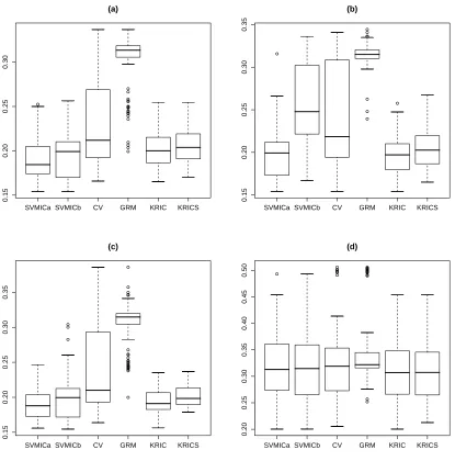
Figure 2 presents the values of the 100 simulated generalization errors as boxplots, giving insight in the variability of the variable selection methods. For most of the cases it turns out that cross-validation is highly variable, while GRM has a small variability. This good property of GRM is, however, accompanied by a much higher average generalization error rate. Comparing the different information criteria shows that SVMICa is quite comparable to the KRICs. The SVMICb has a
larger variability. In the setting with small sample size (n=25) and relatively large number of
variables (100), all methods, except for GRM, are comparable with respect to variability, but GRM has again the largest median error rate. Our main conclusion from this analysis is that SVMICa has a similar variability than the KRIC criteria, but SVMICb has a larger variability. Recall that the average error rates, as reported in Table 1, were of similar magnitude for all the four information criteria. Hence, when needing to choosing between the two newly proposed information criteria, we have a preference for SVMICa.
SVMICa SVMICb CV GRM KRIC KRICS
0.15
0.20
0.25
0.30
(a)
SVMICa SVMICb CV GRM KRIC KRICS
0.15
0.20
0.25
0.30
0.35
(b)
SVMICa SVMICb CV GRM KRIC KRICS
0.15
0.20
0.25
0.30
0.35
(c)
SVMICa SVMICb CV GRM KRIC KRICS
0.20
0.25
0.30
0.35
0.40
0.45
0.50
(d)
Figure 2: Generalization error rates for 100 simulation experiments, for n=100, p=25 (a) linear
kernel, ranking with kwk2, (b) linear kernel, ranking with Fisher score, (c) quadratic
kernel, ranking withkwk2, and for (d) n=25, 100 variables, linear kernel and ranking
withkwk2.
Kernel: Linear Quadratic
Models selected: C U O R C U O R
n=25; p=25 SVMICa 1 22 1 76 3 36 0 61
SVMICb 0 42 0 58 0 64 0 36
CV 0 38 4 58 1 40 5 54
GRM 0 77 0 23 0 75 0 25
KRIC 1 1 7 91 0 1 25 74
KRICS 0 0 9 91 0 0 49 51
n=200; p=25 SVMICa 22 0 76 2 2 0 98 0
SVMICb 77 9 10 4 67 14 6 13
CV 7 48 43 2 4 43 49 4
GRM 1 98 1 0 1 99 0 0
KRIC 6 0 93 1 8 0 84 8
KRICS 1 0 99 0 0 0 100 0
n=25; p=100 SVMICa 0 8 0 92 0 35 0 65
SVMICb 0 20 0 80 0 63 0 37
CV 0 23 6 71 0 33 10 57
GRM 0 56 0 44 0 64 0 36
KRIC 0 1 0 99 0 0 41 59
KRICS 0 0 1 99 0 0 56 44
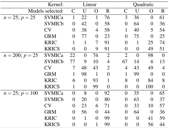
Table 2: Simulated frequencies of selected models, with variable ranking done by influence on kwk2. Here ‘C’ denotes correct selection, ‘U’ is underfitting, ‘O’ is overfitting, and ‘R’ for all other situations.
subset of the important variables, but no irrelevant variables are included. The good performance of SVMICa and SVMICb might be due to the fact that these criteria seem to have the tendency to select a set of variables which includes all significant ones as the number of observations grows. The simulation results indicate that SVMICa behaves like AIC with its tendency to overfit. The SVMICb seems to share the property of BIC that it selects the correct model more often, if at least this true model is one of the possibilities to select from. The cross-validated error rate, and the general risk minimisation in particular, seem to have the tendency to ignore variables which nevertheless are important. As a consequence, the models that these criteria select are of poor predictive quality. The two KRICs of Kobayashi and Komaki (2006) share the overselection property exhibited by SVMICa, but the KRICs select excessive variables even more frequently than SVMICa. This can explain why these criteria perform somewhat worse when the number of observations is large, and why they outperform the proposed SVMICs when the number of observations is small, since the latter tend to underfit the model in the case of few observations.
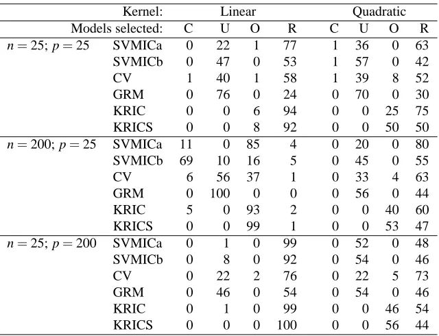
This concludes the results for the case of two populations coming from an identical distribution, differing only in mean. Another case that we examined is where the variances of the two populations differ from each other. We performed a simulation study, in a similar way as the previous one, where the samples have been drawn from
N
(µ,Ip)for class+1, and fromN
(−2µ,4Ip)for class−1.Linear kernel
n p SVMICa SVMICb CV GRM KRIC KRICS
25 25 28.9 28.0 30.1 29.2 30.4 28.4 32.7 31.6 29.0 27.5 28.8 27.7 50 33.3 30.2 34.2 31.3 35.1 31.4 35.3 33.1 32.7 30.7 32.5 30.5 100 35.6 31.5 35.7 32.3 36.0 32.6 36.9 33.7 34.8 32.6 34.8 33.0 200 36.5 33.2 36.4 34.4 36.4 34.2 36.6 35.6 36.4 33.5 36.1 33.7 50 25 23.3 20.5 23.9 21.9 26.1 24.9 28.9 28.6 24.2 23.6 24.6 24.3 50 27.1 21.7 25.7 22.7 27.7 25.2 29.1 28.4 27.7 26.8 27.6 27.1 100 28.3 23.1 27.4 23.7 28.7 25.2 29.9 28.7 28.4 26.7 28.4 27.5 100 25 19.0 17.4 18.1 17.4 22.7 21.5 27.6 27.6 20.5 20.0 21.0 20.9 50 21.8 17.8 19.3 18.0 23.5 22.7 26.9 27.0 24.8 25.0 25.0 25.5 200 25 17.0 16.1 15.9 15.6 21.4 20.7 27.0 27.0 17.9 17.0 18.3 17.8 Quadratic kernel
n p SVMICa SVMICb CV GRM KRIC KRICS
25 25 29.2 28.9 31.8 31.8 31.8 28.7 35.4 34.7 25.7 24.9 25.8 26.2 50 35.1 35.8 39.6 40.0 38.1 37.6 42.8 42.4 30.5 30.8 31.3 32.3 100 42.1 41.7 48.2 48.1 42.2 42.3 49.4 48.7 35.0 36.0 36.2 38.1 200 50.1 50.1 50.1 50.1 44.7 44.4 50.1 50.1 38.9 40.0 40.4 41.8 50 25 20.5 19.3 23.5 22.2 25.9 24.5 30.6 30.2 19.0 19.1 19.5 19.9 50 23.1 22.2 26.1 26.2 28.3 27.6 33.2 32.7 23.8 23.9 25.1 26.1 100 26.5 25.8 30.4 30.4 34.5 33.7 40.5 40.4 28.2 28.8 30.1 32.3 100 25 14.6 15.2 18.5 16.4 20.8 19.9 27.8 27.1 14.2 14.5 14.5 14.9 50 17.9 17.0 18.4 17.8 22.0 21.5 27.7 28.3 18.1 18.5 19.5 20.3 200 25 9.9 9.8 12.9 13.2 19.6 17.6 29.3 26.8 10.1 10.3 9.7 9.8
Table 3: As Table 1, but now for two populations with different variances.
Kernel: Linear Quadratic
Models selected: C U O R C U O R
n=25; p=25 SVMICa 0 22 1 77 1 36 0 63
SVMICb 0 47 0 53 1 57 0 42
CV 1 40 1 58 1 39 8 52
GRM 0 76 0 24 0 70 0 30
KRIC 0 0 6 94 0 0 25 75
KRICS 0 0 8 92 0 0 50 50
n=200; p=25 SVMICa 11 0 85 4 0 20 0 80
SVMICb 69 10 16 5 0 45 0 55
CV 6 56 37 1 0 33 4 63
GRM 0 100 0 0 0 56 0 44
KRIC 5 0 93 2 0 0 40 60
KRICS 0 0 99 1 0 0 53 47
n=25; p=200 SVMICa 0 1 0 99 0 52 0 48
SVMICb 0 8 0 92 0 54 0 46
CV 0 22 2 76 0 22 5 73
GRM 0 46 0 54 0 54 0 46
KRIC 0 1 0 99 0 0 46 54
KRICS 0 0 0 100 0 0 56 44
Table 4: As Table 2, but now for two populations with different variances.
are similar. More precisely, the SVMICs have an improved performance with respect to the KRICs
when the sample size is large (n≥50) and the linear kernel is used, and the KRICs work slightly
the KRICs, which is only matched by SVMICa for larger sample sizes. From Table 4 we can again make the same observations as before when the linear kernel is used. For the quadratic kernel the SVMICs have more difficulty selecting all the relevant variables than the KRICs, which explains why the latter criteria have an improved performance here.
We also conducted a simulation experiment where the input variables were strongly correlated. First, the observations were generated as in the first simulation experiment. Then, we applied the transformation
xi j=ρxikj+εi j withεi j∼
N
(0,ρ2)i.i.d.
where i=1, . . . ,n, kjis chosen arbitrarily between 1 and 4, and 4< j≤p/2, such that about half of the unimportant input variables are correlated with the four important ones. The parameter|ρ|<1
controls the degree of correlation. We have chosenρ=0.8 and found similar results (not reported)
as for the case where the variances of both class-population differ.
5. Tests on Real Data Sets
We compare the performance of the new methods with that of the other discussed criteria on several real-world data sets. We use some of the benchmark data sets used in Rakotomamonjy (2003), and in R¨atsch et al. (2001). The data sets used are the Pima Indians Diabetes database (768 observations, 8 variables), the Statlog Cleveland Heart Disease database (303 observations, 14 variables), and Leo Breiman’s ringnorm and twonorm data sets (both 7400 observations, 20 variables). These data sets are available from the UCI Machine Learning Repository (the first two), and the Delve Repository (last two). We perform 100 random splits of the data in a training sample and a test sample, where
the size of the training sample is chosen as√2n, with n the total number of observations in the data
set. We chose the size of the training set such that there is a sufficient amount of observations in the test sample to estimate the generalization (out-of-sample) error rate. The training sample size is relatively small, such that the computation time for the KRIC remains within bounds. For each of these partitions we perform variable selection on the training sample exactly as in the simulation study. We first rank the variables to retain p stacked subsets of input variables, and then use the information criteria to select the variables that best explain the training data. Then, we predict the class labels for the test sample, and use these predictions to estimate the generalization error rate.
We use variable ranking based on variable influence onkwk2as well as on Fisher score, and we use
a linear, quadratic and radial kernel.
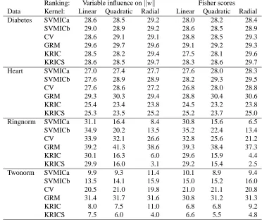
The estimated generalization error rates are presented in Table 5 for each data set and estimation setting. We observe that the KRICs are the preferred choice of variable selection criterion in terms of generalization error rate for the ‘twonorm’ and ‘heart’ data sets. For the ‘ringnorm’ and ‘diabetes’ data sets the difference in performance between the KRICs and our newly proposed SVMICs is less pronounced. The predictive performance of the models selected by SVMICa are for most settings comparable to that of the KRIC, while being much faster to compute. These results are consistent across all settings. The CV error rate and especially the GRM have a poor performance, which is in line of the results obtained in the simulation.
Ranking: Variable influence onkwk Fisher scores Data Kernel: Linear Quadratic Radial Linear Quadratic Radial
Diabetes SVMICa 28.6 28.5 29.2 28.0 28.2 28.4
SVMICb 29.0 28.9 29.2 28.6 28.5 28.9
CV 28.6 29.1 29.1 28.8 28.5 29.3
GRM 29.6 29.7 29.6 29.1 29.2 29.3
KRIC 28.5 28.2 29.4 27.5 28.1 29.6
KRICS 28.6 28.5 29.7 28.3 28.6 29.7
Heart SVMICa 27.0 27.4 27.7 27.6 28.0 28.3
SVMICb 27.6 28.9 28.9 28.2 29.3 29.5
CV 27.6 28.6 27.2 26.8 28.0 28.8
GRM 29.3 30.3 29.4 28.8 30.4 30.6
KRIC 25.4 23.4 23.8 24.5 23.2 23.8
KRICS 25.3 23.5 25.2 25.2 23.7 25.0
Ringnorm SVMICa 31.1 16.4 8.4 30.8 15.6 6.5
SVMICb 34.9 20.2 13.5 35.2 22.4 13.4
CV 33.9 32.1 26.6 32.8 25.6 21.2
GRM 39.2 41.3 38.6 39.3 38.4 37.3
KRIC 30.1 16.3 6.0 29.6 15.9 4.4
KRICS 29.9 16.0 3.1 29.2 15.4 2.5
Twonorm SVMICa 9.9 9.3 11.4 10.1 8.9 9.4
SVMICb 13.5 14.1 15.9 15.0 15.2 16.0
CV 20.5 21.0 19.8 21.0 21.1 20.8
GRM 31.4 31.7 31.6 30.8 31.2 31.3
KRIC 8.0 7.5 11.0 6.8 6.8 9.2
KRICS 7.5 6.0 4.0 6.6 5.5 4.8
Table 5: Generalization error rates (%) for variable selection applied to four data sets. Two variable ranking schemes and three types of kernel are used for each of the criteria.
somewhat improved predictive performance, though with higher computational cost, of the kernel regularization information criterion.
Finally, we applied the newly proposed information criteria for variable selection to two large
data sets, the “Madelon” (n=2000,p=500) and “Arcene” data (n=100,p=10000). These data
6. Conclusions
In this paper we considered the problem of variable selection in support vector machines. We proposed two new information criteria, SVMICa and SVMICb, which allow us to evaluate the suitability of the selected subset of variables for predictive purposes, without much additional com-putational costs. We provided an argumentation for these criteria, linking SVMICa to the KRIC of Kobayashi and Komaki (2006), and justifying SVMICb with the need for a consistent selection criterion. We demonstrated the effectiveness of these criteria in a simulation study, where we com-pared their predictive performance to the KRIC, cross-validation and general risk minimization. Especially for decision functions which are close to an affine function, we found that SVMICa and SVMICb performed the best of all tested criteria, and were also the easiest to compute. For more complicated decision functions, we found that SVMICa still performs well for selecting models with good generalization properties. We repeated the experiment on several real data examples, and the result confirmed the good properties of these newly proposed criteria. In particular we showed that cross-validation criteria are outperformed in generalization error by the new information criteria, where the latter are coming at almost no additional computational cost.
The aim of our paper was to propose an information criterion for a standard SVM. We do not claim that the procedure is outperforming other very advanced feature selection methods, which are not relying on a standard SVM. Obtaining information criteria for other machine learners is an inter-esting topic for future research. Another research question is how suitable the information criteria are for optimal tuning of the regularization and other parameters of the SVM, without necessarily selecting a subset of input variables. Finally, it would be interesting to continue on the theoretical verification of the good performance of our two proposed criteria, and for example try to obtain consistency results for the SVM information criteria.
Acknowledgments
We thank the Editors, Professor Guyon and Professor Alamdari, and the reviewers for their con-structive and insightful comments on the first submitted version of this paper.
References
H. Akaike. Information theory and an extension of the maximum likelihood principle. In B. Petrov and F. Cs´aki, editors, Second International Symposium on Information Theory, pages 267–281. Akad´emiai Kiad´o, Budapest, 1973.
J. Bai and S. Ng. Determining the number of factors in approximate factor models. Econometrica, 70:191–221, 2002.
J. Bi, K. P. Bennett, M. Emrechts, C. M. Breneman, and M. Song. Dimensionality reduction via sparse support vector machines. Journal of Machine Learning Research, 3:1229–1243, 2003.
S.-W. Chen, Z.-R. Li, and X.-Y. Li. Prediction of antifungal activity by support vector machine approach. Journal of molecular structure: THEOCHEM, 731:73–81, 2005.
N. Cristianini and J. Shawe-Taylor. An Introduction to Support Vector Machines and Other Kernel-based Learning Methods. Cambridge University Press, Cambridge, 2000.
J. Fortuna and D. Capson. Improved support vector classification using PCA and ICA feature space modification. Pattern Recognition, 37:1117–1129, 2004.
I. Guyon and A. Elisseeff. An introduction to variable and feature selection. Journal of Machine Learning Research, 3:1157–1182, 2003.
I. Guyon, J. Weston, S. Barnhill, and V. Vapnik. Gene selection for cancer classification using support vector machines. Machine Learning, 46:389–422, 2002.
I. Guyon, S. Gunn, M. Nikravesh, and L. Zadeh. Feature Extraction, Foundations and Applications. Physica-Verlag, Springer, Berlin, 2006.
I. Guyon, J. Li, T. Mader, P. A. Pletscher, G. Schneider, and M. Uhr. Competitive baseline methods set new standards for the NIPS 2003 feature selection benchmark. Pattern Recognition Letters, 28:1438–1444, 2007.
T. J. Hastie, R. J. Tibshirani, and J. Friedman. The Elements of Statistical Learning: Data Mining, Inference, and Prediction. Springer-Verlag, Heidelberg, 2001.
D. Haughton. On the choice of a model to fit data from an exponential family. The Annals of Statistics, 16:342–355, 1988.
D. Haughton. Size of the error in the choice of a model to fit data from an exponential family. Sankhy¯a, Series A, 51:45–58, 1989.
M. Kearns, Y. Mansour, A. Y. NG, and D. Ron. Experimental and theoretical comparison of model selection methods. Machine Learning, 27:7–50, 1997.
K. Kobayashi and F. Komaki. Information criteria for support vector machines. IEEE Transactions on Neural Networks, 17:571–577, 2006.
Y. Lee, Y. Kim, S. Lee, and J.-Y. Koo. Structured multicategory support vector machines with analysis of variance decomposition. Biometrika, 93:555–571, 2006.
Y. Lin and H. H. Zhang. Component selection and smoothing in multivariate nonparametric regres-sion. Annals of Statistics, 34:2272–2297, 2006.
J. Neumann, C. Schn ¨orr, and G. Steidl. Combined SVM-based feature selection and classification. Machine Learning, 61:129–150, 2005.
H. Peng, F. Long, and C. Ding. Feature selection based on mutual information: Criteria of max-dependency, max-relevance, and min-redundancy. IEEE transactions on Pattern Analysis and Machine Intelligence, 27:1226–1238, 2005.
G. R¨atsch, T. Onoda, and K.-R. M ¨uller. Soft margins for adaboost. Machine Learning, 42:287–320, 2001.
J. Rissanen. Stochastic Complexity in Statistical Inquiry. World Scientific Publishing Co. Inc., Teaneck, NJ, 1989.
B. Sch¨olkopf and A. J. Smola. Learning with Kernels. MIT Press, Cambridge, 2002.
G. Schwarz. Estimating the dimension of a model. The Annals of Statistics, 6:461–464, 1978.
F. Y. Shih and S. Cheng. Improved feature reduction in input and feature spaces. Pattern Recogni-tion, 38:651–659, 2005.
P. Sollich. Bayesian methods for support vector machines: evidence and predictive class probabili-ties. Machine Learning, 46:21–52, 2002.
V. N. Vapnik. Estimation of Dependences Based on Empirical Data. Springer, New York, 1982.
L. Wang, J. Zhu, and H. Zou. The doubly regularized support vector machine. Statistica Sinica, 16: 589–615, 2006.
M. Woodroofe. On model selection and the arc sine laws. The Annals of Statistics, 10:1182–1194, 1982.
H. H. Zhang. Variable selection for SVM via smoothing spline ANOVA. Statistica Sinica, 16: 659–674, 2006.
X. Zhang, X. Lu, Q. Shi, X.-Q. Xu, H.-C. E. Leung, L. N. Harris, J. D. Iglehart, A. Miron, J. S. Liu, and W. H. Wong. Recursive SVM feature selection and sample classification for mass-spectrometry and microarray data. BMC Bioinformatics, 7:197, 2006.