Numerical Methods for Information Tracking of Noisy and Non-smooth Data in Large-scale Statistics

(1)

_____________________________________________________________________________________________________ *Corresponding author: Email: [email protected];

6(4): 1-16, 2019; Article no.JERR.50581

Numerical Methods for Information Tracking of

Noisy and Non-smooth Data in Large-scale

Statistics

B. S. Avinash

1*

, T. Srisupattarawanit

1

and H. Ostermeyer

1

1_{Institute for Dynamics and Vibration, Technical University of Braunschweig, Germany.}

Authors’ contributions

This work was carried out in collaboration among all authors. Author BSA managed the literature search for the present review article and wrote the first draft of the manuscript. Authors TS and HO assisted in the arrangement of article and finalized the draft. All the authors read and approved the final manuscript.

Article Information

DOI: 10.9734/JERR/2019/v6i416957 Editor(s): (1) Dr. P. Elangovan, Associate Professor, Department of EEE, Sreenivasa Institute of Technology and Management Studies, Chittoor, Andhra Pradesh, India.

Reviewers: (1) A. Ayeshamariam, Khadir Mohideen College, India. (2) Hlaing Htake Khaung Tin, University of Computer Studies Yangon, Myanmar.

Complete Peer review History:http://www.sdiarticle3.com/review-history/50581

Received 16 May 2019 Accepted 08 August 2019 Published 16 August 2019

ABSTRACT

In our universe, there is a presence of random bit of disorder in every field that has to be contemplated and understood clearly. This random bit of disorder in a physical system is known as noise. Noise in the field of statistics can be defined as an additional meaningless information that cannot be clearly interpreted which is present in the entire dataset. In large-scale statistics, noisy data has an adverse effect on the results and it can lead to skewness in any data analysis process, if not properly understood or handled. The adverse effect on the results is mainly due to uncorrelated (zero autocorrelation) property of noise. This makes it completely unpredictable at any given point in time, hence thorough investigation and removal of noise plays a vital role in data analysis process. In the field of engineering, measurement of experimental data obtained by using scientific instruments consists of some values that are independent of the experimental setup. One of most widely technique is the optimization methods viz, gradient descent, conjugate gradient, Newton’s method etc. Most of these methods require the determination of derivative of a function specified by the dataset (using finite-difference approximation). If the noisy data is approximated

(2)

Avinash et al.; JERR, 6(4): 1-16, 2019; Article no.JERR.50581

using a specific finite difference method this results in the amplification of noise present in the data. In order to overcome the aforementioned problem of amplification of noise in the derivative of a function, various regularization methods are employed. The parameter that plays a vital role in these methods are termed as regularization parameter. One of the most important technique used in the field of regularization is known as total variation regularization. This review aimed at gathering the disperse literature on the current state of various noises and their regularization methods.

Keywords: Large-scale statistics; noisy data; regularization; data driven methods; amplification.

1. INTRODUCTION

In the modern field of engineering, we deal with a lot of experimental data that may consists of errors. These errors possess the properties of randomness and non-correlation meaning that they are completely unpredictable in nature. Hence the knowledge behind these errors, proper handling and removal techniques are prioritized during the early phase of data analysis [1]. Various numerical method for approximating the derivative of functions like finite-difference methods have taken center stage in many engineering interdisciplinary for optimization purposes. Application of these finite-difference methods to the noise contaminated dataset leads to the amplification of already present noise. These amplification in the derivatives can be suppressed by applying total variation (TV) regularization technique. TV deals directly with the process of differentiation. This process of

regularization assures that the calculated

derivative of the function adheres to a certain

degree of regularity [2]. The successful

implementation of this methods hinges on one

aspect, i.e., clearly understanding and

determination of regularization parameter.

There are various methods that facilitates the determination of optimal regularization parameter One of the most important and widely used is the

L-curve method. This method provides

information on the regularization parameter based on the residual norm (L2) and the solution norm (L1) [3]. The graphical representation between the two for different regularization parameter provides an intersection point that stabilizes the effect of both the residual and the solution. This point is chosen as the optimal regularization parameter by using curvature plot [4].

A method that completely focuses on extensive analysis of residual vector is the normalized cumulative periodogram [5]. The selection of optimal regularization parameter is based on Kolmogorov-Smirnov test i.e., the cumulative

periodogram must strictly lie within the

confidence interval of 95% [6]. In these circumstances, the user is generally in a tough spot. Hence the generalized cross validation method is employed to overcome complexities of unknown exact data or the variance of noise [7].

These optimal parameters can then be used in the data-driven (sparse regression) method in order to determine the PDE of the governing equation. This method provides good approximation of the system as this uses brute-force search and the sparse regression technique for sparse nonlinear time series matrix in order to achieve its goal [8]. With this background, an attempt has been made in this study to investigate the implications of noisy data in large scale statistics and regularization of noisy data in order to retrieve vital information.

2. GENERAL CONSIDERATION

Raw data collection, different types of noise present in a general system, processing and regularization are the important steps of this study. There are many regularization methods, few of the commonly used in the field of signal processing are: Ridge regression; Least Absolute Shrinkage and Selection Operator (LASSO) and Total Variation Regularization or Rudin–Osher– Fatemi model. The collected data must then be organized for future analysis. This process of organization of collected data is known as data processing. Example of data processing is the placement of data into columns and rows with respective variable names in a statistical software (Microsoft® Excel or Minitab™).

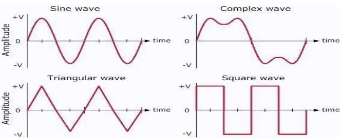
2.1 Different Types of Noise Present In a General System

(3)

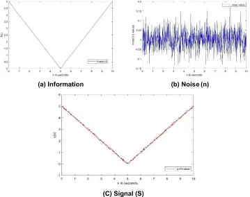
s = i + n

where, s = Signal; i = Information and n = Noise.

2.2.Data Analysis and Steps Involved In The Process

The process of obtaining raw data and its conversion into information which is useful for decision-making by the user, this is known as data analysis. The various steps involved in data analysis are shown in Fig. 2.

2.2.1 Data collection and processing

Data in general can be collected from various number of sources. Digital sources of data collection are some of the most convenient and

trusted forms. In today’s world where

technological advancement is at its peak, sensors form a large part of data collection [9]. They are reliable, accurate and can transmit data round-the-clock to computers which can then be analyzed by the engineers. Temperature sensors in nuclear power plants, on aircraft to monitor engine temperature, seismic sensors in high

earthquake prone regions in world are few examples that can provide engineers and scientists’ accurate data that can save lives during critical situations.

The collected data must then be organized for future analysis. This process of organization of collected data is known as data processing. Example of data processing is the placement of data into columns and rows with respective

variable names in a statistical software

(Microsoft® Excel or Minitab™).

2.2.2 Cleaning of processed data

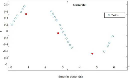
Data cleaning (cleansing) is the process of understanding, collection and then removal of errors that may be present in the processed data [10]. This process is very critical during the final step of data analysis as it improves the accuracy of results. When dealing with quantitative processed data using various outlier removal methods forms the part of data cleaning. Outliers are values or observation in processed data that lie far part from the main pattern of the entire dataset. Fig. 2 shows a process with (Fig. 2a and without outliers 2b).

(a) Information (b) Noise (n)

(C) Signal (S)

(4)

Fig. 2. A picture showing the steps involved in data analysis

Fig. 3. Representation of Outliers in a process

Avinash et al.; JERR, 6(4): 1-16, 2019; Article no.

A picture showing the steps involved in data analysis

Time in seconds (s)

(a) Graph Outlier

Time in seconds (s)

(b) Graph without outlier

Fig. 3. Representation of Outliers in a process

(5)

There are various methods to detect outliers in a process, one of the most commonly used technique is the scatterplot. This is very easy and quick process to detect the number of points lying outside the standard pattern of the whole process (Fig. 3).

There are many other techniques like the box plot that are used in the detection of outliers in a process. The advantage of using box plot is that it provides clear information on mild and extreme outliers. Box plot also has the option of detecting

outliers by using median, 1st and 3rd quartile principle. A typical boxplot is shown in Fig. 5.

After the detection of outliers, one cannot simply employ univariate and multivariate methods to remove the detected outliers as it can have adverse effect on the entire process. So using robust techniques like "Minkowski error" method helps to reduce the impact of outliers on the

dataset (or model). The major advantage of "Minkowski error" over RSS is that it reduces the effect of outliers by taking the power of error terms lesser than 2 [11].

In certain scenarios, processed data and/or processed data after treating outliers may be skewed. This type of skewed data needs to be

transformed using certain transformation

techniques before analyzing exploratory. The most common method employed for skewed data is the Box- Cox (or power) transformation.

x(λ) =(xλ −1) λ = 0 (2.2)

Λ

x(λ) = ln(x) λ = 0 (2.3)

where, x(λ) = Transformed data; x = Skewed data; λ = Box-Cox parameter.

Fig. 4. A scatterplot showing the process trend and the detected outliers

(6)

But the best way [12] to select “λ" is by using LLF (logarithm of likelihood function). This

marks the conclusion of cleansing of

processed data.

2.2.3 Exploratory data analysis

The process of deciphering the cleaned data extensively by using visualization techniques, calculation of vital descriptive statistics (like mean, median, mode etc.) is known as exploratory data analysis. This helps the user to comprehend the meaning behind the obtained dataset. Hence it translates to exploring the cleaning data from all possible angles. It consists of many sub-tasks like, re-cleansing (if necessary), procurement of

additional data, calculation of descriptive

statistics and visualization.

2.2.4 Data modeling

The final step in process of data analysis is data

modeling. The knowledge obtained from

exploratory data analysis steps plays a vital role in the identification of certain relationship between variables. Various relationships such as regression analysis, correlation can be obtained by compiling specific algorithms and/or applying specific mathematical formulae. Finally, the user can construct descriptive models for analysis [13]. The results obtained can be termed as information, this can help the user to understand the datasets and certain changes can be made in order to improve the efficiency of the process for future studies.

3. A BRIEF DISCUSSION ABOUT NOISE

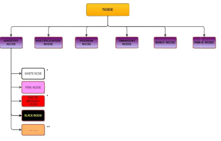
This section focuses on the different types of noise and its characteristics encountered in various statistical and signal processing fields. As shown in equation 2.1, noise "n" can be classified as shown below,

3.1 Different Types of Noise

(Fig. 6) are explained [14]:

Multiplicative noise: In a given system, if the random term depends on the state of that system, this type of noise is termed as multiplicative noise. In terms of dataset, we can say that the noisy data is the resultant of noise multiplied to the data vector. This can be clearly interpreted with the help of a following system (model).

s = i · n (2.4)

where s= Signal; i=Information (true signal) and n=Noise

Denoising of multiplicative noise requires a transformation of the model in equation 2.4 into additive noise. Logarithmic transformation is very helpful tool in denoising multiplicative noise as this provides an additive form.

log(s) = log (i · n) (2.5)

log(s) = log(i) + log(n) (2.6)

where s =Signal; i=Information(true signal) and n=Noise.

Now, equation 2.6 clearly represents an

additive system and various denoising

techniques can be applied. Finally, inverse

logarithm (log-1) of the denoised signal

provides the solution to the original system.

Poisson Noise: Poisson noise is also termed as shot noise (Fig. 7). Shot noise is

mainly observed in electronic devices.

This type of noise is generated when a charge carrier such as electrons or ions travel through a gap results in random fluctuation in electric current. This random fluctuation is known as shot noise [15].

Transient Noise: This type of noise is very common in the field of communication systems like mobile phones and hearing aids. The background noise that hinders communication in the field of communication systems is termed as transient noise (Fig. 8).

Burst Noise: Burst noise is also termed as Random Telegraph Signal (RTS) and “popcorn” noise. It is very similar to the shot noise and generated at low frequencies. When a single charger carrier is captured by a single trapping center, this leads to the generation of burst noise as shown in Fig. 9.

(7)

Note: As seen from Fig.

(∗∗) =⇒ additive noise includes many other slightly less significant subdivision

3.2 Additive White Gaussian Noise

(AWGN)

Before jumping into the deep end

regarding the explanation of AWGN, let us first break down and understand the terminology "Additive White Gaussian Noise".

Additive = ⇒This type of noise are additive in nature. This means that the received signal is

Fig. 6. Classification of noise

Fig. 6; (∗) =⇒ main focal point. Hence it is explicitly described in

additive noise includes many other slightly less significant subdivision

Fig. 7. Poisson noise

Additive White Gaussian Noise

Before jumping into the deep end

regarding the explanation of AWGN, let us first break down and understand the terminology

This type of noise are additive in nature. This means that the received signal is

the resultant of information added with some noise as shown in equation 2.1.

White =⇒ It is mixture of all types or colors of noise. White light is mixture o

frequencies or wavelength of visible

spectrum (shown in Fig. 11). This definition of white light is literally translated into white noise [16].

; Article no.JERR.50581

focal point. Hence it is explicitly described in 3.3.

the resultant of information added with some

It is mixture of all types or colors of noise. White light is mixture of all the

frequencies or wavelength of visible

(8)

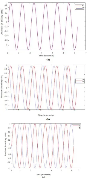
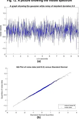
Gaussian = ⇒This type of noise follows normal probability distribution Function (pdf), classified as shown in Fig. 12.

White noise with respect to a signal and its source is a statistical model having constant

power spectral density (PSD), which means that it is a random noise having equal

intensity for different frequencies. An

example of the Gaussian white noise is shown in Fig. 13.

Fig. 8. Transient noise

Fig. 9. A graph showing the generation of pop (burst) noise

(9)

(10)

Fig. 12. A picture showing the visible spectrum

(a)

(b)

(11)

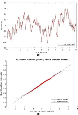
Brownian Noise: Brownian noise [17] is also known as red Noise. Longer wavelength produces stronger noise similar to radio waves shown in Fig.14, hence the term "red" noise. Robert Brown discovered Brownian motion. Hence it’s also coined as "brown" noise.

The characteristics of red noise are briefly discussed below, Red noise has more energy

at lower frequencies =⇒P (f)∝1/f2. Power

spectrum is denoted by P (f). Frequency is denoted by f Integration of white noise → Red noise.

An example of the Brownian or red noise is shown below,

With this brief understanding of different types of noise, let us now dive into the concepts surrounding important regularization methods.

3.3 A Brief Discussion Regarding

Regularization Methods

As mentioned earlier, the 3 widely used regularization techniques are:

1. Ridge regression or Tikhonov

regularization method

2. Least Absolute Shrinkage and Selection Operator (LASSO)

3. Total Variation Regularization or Rudin– Osher–Fatemimodel

Before we step into each of the

aforementioned regularization techniques, let us define the term regularization. Regularization is defined as a method that helps to overcome the problem surrounding over-fitting of penalized regularization coefficients [18]. This aim of regularization is achieved by the introduction of

additional information to solve ill-poised

problems. Due to the fact that minimization of residual sum square are highly unstable in nature, regularization methods proves to be all the more important in many scientific fields.

Ridge regression (L2 regularization): The aim of ridge regression is to minimize the

ordinary least square with an added

penalty term. This penalty term is the square of

the magnitude of the coefficients. This

explanation is summarized in equation 2.8.

The ridge regression solution "xˆridge" solves the following minimization problem for a given system Ax = b,

(2.7)

The equation 2.7 can be represented in a simpler form as,

(2.8)

Where,

b ∈ Rn = Response vector;

A ∈ Rn×m = Predictor matrix

α = Regularization parameter

In matrix notation equation 2.8 becomes,

Cridge = (A x − b) T (A x − b) + α xT x (2.9)

Expanding and simultaneous simplification of equation 2.9 results in the following [7].

Cridge = xT AT A x − bT A x − xT AT b + bT b + α xT x (2.10)

= x

T

AT A x − x

T

AT b − x

T

AT b + bT b + xT αI x (2.11)

= b

T

b − 2 xT AT b + xT AT A x + xT αI x (2.12)

Cridge = bT b − 2 xT AT b + xT (AT A + αI)x (2.13)

The objective function in 2.7 can be minimized by taking the partial derivative of 2.13 with respect to "x”.

Minimization condition =⇒ the gradient of the objective function must be equal to zero.

(12)

∗ indicates that the specific part of the

(symmetric) differentiation

Simplification of the equation 2.16 le

where,

I = Identity matrix (n × m); α I = Ridge term

Advantages ridge term,

i) Facilitates invertibility of resultant gets added to the principle diagonal. ii) Consistently achieves a unique solution

The equation 2.8 can be interpreted

geometrically as shown in Fig. 15:

The Fig.15 clearly depicts the aim of ridge (L2 regularization) regression i.e., minimization

occurs simultaneously between the RSS

(ellipse) and the penalty term (circle) mentioned in equation 2.8. The simultaneous

occurs at "xˆridge" shown in equation

Lasso: LASSO aims to minimize least square with an added penalty

case of L1- regularization, the penalty term is the sum of the absolute value of the regression coefficients. Hence LASSO is also known L1-regularization [21].

where, b ∈ Rn = Response vector; A Predictor matrix; α = Regularization parameter

The first part of the derivation is similar to regularization, in matrix notation equation 2.8 becomes,

α

the equation was achieved by successfully applying matrix (symmetric) differentiation rule

eads to the ridge regression solution i.e., "xˆridge"

α I = Ridge term

resultant matrix and it .

solution.

clearly depicts the aim of ridge (L2-regularization) regression i.e., minimization

occurs simultaneously between the RSS

(ellipse) and the penalty term (circle) mentioned minimization tion 2.17.

the ordinary penalty term [20]. In penalty term is the sum of the absolute value of the regression known as the

(2.18)

The equation 2.7 can be represented in a

(2.19)

Rn = Response vector; A ∈ Rn×m = Predictor matrix; α = Regularization parameter

The first part of the derivation is similar to L2-regularization, in matrix notation equation 2.8

Classo = (A x − b)T (A x − b) +α |x|

Expanding and simultaneous simplification of equation 2.20 results in the following,

Classo = xT AT A x − bT A x − x

α |x|1

= xT AT A x − xT AT b − xT AT b + b Classo = bT b − 2 xT AT b + xT A

where,

b ∈ Rn = Response vector; A

Predictor matrix; α = Regularization parameter

The first part of the derivation is similar to L2 regularization, in matrix notation equation 2.8 becomes,

Classo = (A x − b)T (A x − b) +α |x|

Expanding and simultaneous simplification equation 2.23 results in the following,

Classo = xT AT A x − bT A x − x

α |x|1

= x

T

AT A x − x

T

AT b − xT AT b + Classo

= bT b − 2 xT AT b + xT AT A x

Next, taking the derivative of equation 2.26, we get,

∇Classo = −2AT b + 2AT Ax + ∇(α |x|

(2.17) (2.15)

(2.16)

α |x|1 (2.20)

Expanding and simultaneous simplification of equation 2.20 results in the following,

− xT AT b + bT b + (2.21)

b + bT b + α |x|1

AT A x + α |x|1

The equation 2.7 can be represented in a simpler

(2.22)

= Response vector; A ∈ Rn×m =

Predictor matrix; α = Regularization parameter.

The first part of the derivation is similar to L2-regularization, in matrix notation equation 2.8

α |x|1 (2.23)

simplification of following,

xT AT b + bT b +

(2.24)

+ b

T

b + α |x|1

(2.25)

+ α |x|1 (2.26)

Next, taking the derivative of equation 2.26, we

(13)

(a)

(b)

Fig. 14. Representation of Brownian/red noise and its quantile-quantile plot

(14)

Due the face that equation 2.24 consists of the term "∇(α |x|1)", sub-differential helps us to arrive at the final solution. But before we step into sub-differential, let us assume that the ATA is equal to I and multiply "2" to the penalty term.

Equation 2.27 becomes,

∇Classo = −2AT b + 2x + 2∇(α

Now, the sub-differential becomes,

Breaking down each of the 3 conditions mentioned in equation 2.29,

Case 1: when x > 2x − 2AT b + 2α = 0

Equation 2.30 must be satisfied.

Therefore, we get, x = 2AT b –

Case 2: when x = 0

0 ∈ [−2α, 2α] − 2AT b

Therefore, we now have 2 sub-cases, i.e,

−2α − 2AT b < 0 =⇒ α > −AT b

Fig. 16. Geometric representation of LASSO regression [22]

Due the face that equation 2.24 consists of the differential helps us to

arrive at the final solution. But before we differential, let us assume that the

is equal to I and multiply "2" to the penalty

(α |x|1) (2.28)

(2.29)

Breaking down each of the 3 conditions

b + 2α = 0 (2.30)

– α (2.31)

(2.32)

cases, i.e,

(2.33)

2α − 2AT b > 0 =⇒ α > AT b

The sub-cases mentioned in equation 2.34 becomes,

α > AT b

when x = 0

Case 3: when x < 2x − AT b− 2α = 0

Equation 2.36 must be satisfied. Therefore, we get,

x = AT b + α

The aforementioned cases help us to a the solution for LASSO and it summarized in the equation below,

geometrically as shown in Fig. 16:

The Fig.16 clearly depicts the aim of LASSO (L1

regularization) regression i.e., minimization

occurs simultaneously between the RSS (circle) and the penalty term (square) mentioned in equation 2.19. The simultaneous minimization occurs at “xlasso” shown in equation

Geometric representation of LASSO regression [22]

(2.34)

cases mentioned in equation 2.34

(2.35)

α = 0 (2.36)

Equation 2.36 must be satisfied. Therefore, we

(2.37)

The aforementioned cases help us to arrive at the solution for LASSO and it summarized in the

(2.38)

clearly depicts the aim of LASSO

(L1-regularization) regression i.e., minimization

occurs simultaneously between the RSS (circle) and the penalty term (square) mentioned in equation 2.19. The simultaneous minimization

(15)

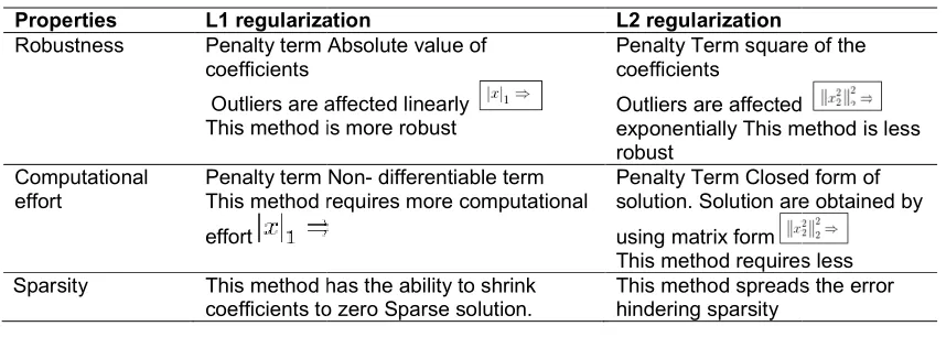
Table 1. Comparison between L1 and L2 regularization

Properties L1 regularization

Robustness Penalty term Absolute value of

coefficients

Outliers are affected linearly This method is more robust

Computational effort

Penalty term

This method requires more computational

effort

Sparsity This method has the ability to shrink

coefficients to zero Sparse solution.

4. CONCLUSION

The fundamentals of large-scale statistics was focused with retrieving the information from noisy data in the present review article. The method of total variation regularization helps to study thoroughly and understand the concept behind

regularization parameter on various test

functions each at different amplitude of noise. The study behind the optimal parameter value shines light on the fact that a stronger noise level in a large-scale dataset requires considerably strong optimal parameter. As we know that, in the real-life problems it is very difﬁc

noise from the actual measurement data which needs the iterative process to automatically obtain regularization parameter. The information being tracked was implemented in the process of ﬁnding differential equations by using data (or Sparse Regression) method.

COMPETING INTERESTS

Authors have declared that no competing interests exist.

REFERENCES

1. Rani NS, Rao PS, Anurag. Study an

analysis of noise effect on big data analytics.Int. J. Management, Te

and Engineering. 2018;8(XII):5841

2. Chartrand R. Numerical differentiation of

noisy, no smooth data. ISRN Applied Mathematics. 2011;1–11.

DOI:10.5402/2011/164564

3. Hansen PC. Analysis of discrete ill problems by means of the l Review. 1992;34(4):561–580.

4. Belge M, Kilmer ME, Miller EL.

determination of multiple regularization

Table 1. Comparison between L1 and L2 regularization

L1 regularization L2 regularization

Penalty term Absolute value of

Outliers are affected linearly This method is more robust

Penalty Term square of the coefficients

Outliers are affected

exponentially This method is less robust

Non- differentiable term This method requires more computational

Penalty Term Closed form of solution. Solution are obtained by

using matrix form

This method requires less This method has the ability to shrink

coefficients to zero Sparse solution.

This method spreads the error hindering sparsity

scale statistics was focused with retrieving the information from noisy data in the present review article. The method of total variation regularization helps to study thoroughly and understand the concept behind

regularization parameter on various test

erent amplitude of noise. The study behind the optimal parameter value shines light on the fact that a stronger noise level scale dataset requires considerably strong optimal parameter. As we know that, in ficult to define noise from the actual measurement data which needs the iterative process to automatically obtain regularization parameter. The information being tracked was implemented in the process of finding differential equations by using data-driven

Authors have declared that no competing

Rani NS, Rao PS, Anurag. Study an analysis of noise effect on big data analytics.Int. J. Management, Technology

(XII):5841-5850. Chartrand R. Numerical differentiation of noisy, no smooth data. ISRN Applied

Hansen PC. Analysis of discrete ill-posed the l-curve. SIAM

580.

Belge M, Kilmer ME, Miller EL. Efficient determination of multiple regularization

parameters in a generalized l framework. Inverse problems. 2002;18(4): 1161–1183.

5. Hansen PC. Kilmer ME. A parameter

choice method that exploits re information. PAMM. 2007;

1021706.

6. Rust BW, Dianne PO. Residual

periodograms for choosing regularization parameters for ill-posed problems. Inverse Problems. 2008;24(3):034005.

7. Jansen M, Malfait M, Bultheel A.

Generalized cross validation for wavelet thresholding. Signal Processing. 1 56(1):33–44.

8. Rudy SH, Brunton SL, Proctor JL, Kutz JN.

Data-driven discovery of partial differential equations. Science Advances. 2017; e1602614.

9. Hariri RH, Fredericks EM, Bowers KM.

Uncertainity in big data analysis: Sur opportunities and challenges. J.Big Data. 2019;6:44.

Available:https://doi.org/10.1186/s40537 019-0206-3

10. Kumar RK, Chadrasekaran RM. Attribute

correction-data cleaning using association rule and clustering methods. Int. J. Data

Mining & Knowledge Mana

Process. 2011;1(2):22-32.

11. Ogu AI, Inyama SC, Achugamonu PC.

Methods of Detecting Outliers in A Regression Analysis Model. West African J. Industrial and Academic Research. 2013;7(1):105-113.

12. Martinez WL, Martinez AR, Solka J.

Exploratory Data Analysis with MATLAB, Second Edition. Chapman & Hall/CRC; 2010.

[ISBN 9781439812204]

Penalty Term square of the

Outliers are affected

exponentially This method is less

Penalty Term Closed form of Solution are obtained by

This method requires less This method spreads the error

parameters in a generalized l-curve mework. Inverse problems. 2002;18(4):

Hansen PC. Kilmer ME. A parameter-choice method that exploits residual

MM. 2007;7(1):1021705–

Rust BW, Dianne PO. Residual

periodograms for choosing regularization oblems. Inverse 24(3):034005.

Jansen M, Malfait M, Bultheel A.

Generalized cross validation for wavelet ing. Signal Processing. 1997;

runton SL, Proctor JL, Kutz JN. driven discovery of partial differential ations. Science Advances. 2017;3(4):

Hariri RH, Fredericks EM, Bowers KM. Uncertainity in big data analysis: Survey, hallenges. J.Big Data.

i.org/10.1186/s40537-Kumar RK, Chadrasekaran RM. Attribute data cleaning using association rule and clustering methods. Int. J. Data

ledge Management

Ogu AI, Inyama SC, Achugamonu PC. Methods of Detecting Outliers in A Regression Analysis Model. West African Academic Research.

(16)

13. Mahmoudi A. Adaptive Algorithm for

Estimation of Two-Dimensional

Autoregressive Fields from Noisy

Observations. Int. J. Stochastic Analysis. 2014;7.

[Article ID: 502406]

14. Alexander Ch. Sadiku M, Fundamentals of

electric circuits. Fifth Edition. McGraw- Hill; 2013.

15. Bubba TA, Porta F, Zanghirati G, Bonettini

S. A nonsmooth regularisation approach based on shearlets for Poisson noise removal of ROI tomography. Applied Mathematics and Computation. 2018;318: 131-152

16. Sliney DH. What is light? The visible

spectrum and beyond. Eye (Lond). 2016; 30(2):222–229.

17. Song S, Chandhuri K, Sarwate AD.

Learning from data with heterogeneous noise using SGD. JMLR Workshop Conf.Proc. 2015;894-902

18. Srivastava N, Hinton G, Krizhevsky A,

Sutskeverilya E, Salakhutdinov R.

Dropout: A simple way to prevent neural networks from over fitting. J. Machine Learning Research. 2014;15:1929-1958.

19. Wieringen WNV, Lecture notes on ridge

regression – version 0.20; 2018.

Available: https://arxiv.org/pdf/1509.09169

20. Chang H, Zhang D. Machine learning

subsurface flow equations from data. Computational Geosciences; 2019. Available:http://doing.org/10.1007/s10596-019-09847-2

21. Hastie T, Tibshirani R, Wainwright M.

Statistical Learning with Sparsity: The Lasso and Generalizations, CRC Press; 2015.

22. Jiang Y, Yunxiao H, Zhang H. Variable

selection with prior information for

generalized linear models is the prior lasso

method. J. American Statistical

Association. 2016;111(513):355–376.

© 2019 Avinash et al.; This is an Open Access article distributed under the terms of the Creative Commons Attribution License (http://creativecommons.org/licenses/by/4.0), which permits unrestricted use, distribution, and reproduction in any medium, provided the original work is properly cited.

Peer-review history: