Nonlinear Models Using Dirichlet Process Mixtures
Babak Shahbaba [email protected]
Department of Statistics
University of California at Irvine Irvine, CA, USA
Radford Neal [email protected]
Departments of Statistics and Computer Science University of Toronto
Toronto, ON, Canada
Editor: Zoubin Ghahramani
Abstract
We introduce a new nonlinear model for classification, in which we model the joint distribution of response variable, y, and covariates, x, non-parametrically using Dirichlet process mixtures. We keep the relationship between y and x linear within each component of the mixture. The overall relationship becomes nonlinear if the mixture contains more than one component, with different regression coefficients. We use simulated data to compare the performance of this new approach to alternative methods such as multinomial logit (MNL) models, decision trees, and support vector machines. We also evaluate our approach on two classification problems: identifying the folding class of protein sequences and detecting Parkinson’s disease. Our model can sometimes improve predictive accuracy. Moreover, by grouping observations into sub-populations (i.e., mixture com-ponents), our model can sometimes provide insight into hidden structure in the data.
Keywords: mixture models, Dirichlet process, classification
1. Introduction
In regression and classification models, estimation of parameters and interpretation of results are easier if we assume that distributions have simple forms (e.g., normal) and that the relationship between a response variable and covariates is linear. However, the performance of such a model depends on the appropriateness of these assumptions. Poor performance may result from assum-ing wrong distributions, or regardassum-ing relationships as linear when they are not. In this paper, we introduce a new model based on a Dirichlet process mixture of simple distributions, which is more flexible in capturing nonlinear relationships.
A Dirichlet process,
D
(G0,γ), with baseline distribution G0 and scale parameter γ, is a dis-tribution over disdis-tributions. Ferguson (1973) introduced the Dirichlet process as a class of prior distributions for which the support is large, and the posterior distribution is manageable analyti-cally. Using the Polya urn scheme, Blackwell and MacQueen (1973) showed that the distributions sampled from a Dirichlet process are discrete almost surely.unknown distribution. We can model the distribution of y as a mixture of simple distributions, with probability or density function
P(y) =
C
∑
c=1
pcF(y,φc).
Here, pcare the mixing proportions, and F(y,φ)is the probability or density for y under a
distribu-tion, F(φ), in some simple class with parametersφ—for example, a normal in whichφ= (µ,σ). We first assume that the number of mixing components, C, is finite. In this case, a common prior for pc
is a symmetric Dirichlet distribution, with density function
P(p1, ...,pC) =
Γ(γ) Γ(γ/C)C
C
∏
c=1
p(cγ/C)−1,
where pc ≥0 and∑pc =1. The parametersφc are independent under the prior, with distribution
G0. We can use mixture identifiers, ci, and represent this model as follows:
yi|ci,φ ∼ F(φci),
ci|p1, ...,pC ∼ Discrete(p1, ...,pC),
p1, ...,pC ∼ Dirichlet(γ/C, ....,γ/C),
φc ∼ G0.
(1)
By integrating over the Dirichlet prior, we can eliminate the mixing proportions, pc, and obtain the
following conditional distribution for ci:
P(ci=c|c1, ...,ci−1) =
nic+γ/C
i−1+γ. (2)
Here, nicrepresents the number of data points previously (i.e., before the ith) assigned to component
c. As we can see, the above probability becomes higher as nicincreases.
When C goes to infinity, the conditional probabilities (2) reach the following limits:
P(ci=c|c1, ...,ci−1) →
nic
i−1+γ,
P(ci6=cj for all j<i|c1, ...,ci−1) → γ i−1+γ.
As a result, the conditional probability forθi, whereθi=φci, becomes
θi|θ1, ...,θi−1 ∼ 1
i−1+γ
∑
j<iδθj+γ
i−1+γG0, (3)
whereδθis a point mass distribution atθ. Since the observations are assumed to be exchangeable, we can regard any observation, i, as the last observation and write the conditional probability ofθi
given the otherθjfor j6=i (writtenθ−i) as follows:
θi|θ−i ∼
1
n−1+γ
∑
j6=iδθj +γ
The above conditional probabilities are equivalent to the conditional probabilities forθiaccording
to the Dirichlet process mixture model (as presented by Blackwell and MacQueen, 1973, using the Polya urn scheme), which has the following form:
yi|θi ∼ F(θi),
θi|G ∼ G, (5)
G ∼
D
(G0,γ).That is, If we let θi =φci, the limit of model (1) as C→∞becomes equivalent to the Dirichlet
process mixture model (Ferguson, 1983; Neal, 2000). In model (5), G is the distribution overθ’s, and has a Dirichlet process prior,
D
. Phrased this way, each data point, i, has its own parameters, θi, drawn independently from a distribution that is drawn from a Dirichlet process prior. But sincedistributions drawn from a Dirichlet process are discrete (almost surely) as shown by Blackwell and MacQueen (1973), theθifor different data points may be the same.
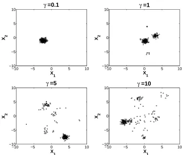
The parameters of the Dirichlet process prior are G0, a distribution from whichθ’s are sampled, andγ, a positive scale parameter that controls the number of components of the mixture that will be represented in the sample, such that a larger γ results in a larger number of components. To illustrate the effect ofγon the number of mixture components in a sample of size 200, we generated samples from four different Dirichlet process priors withγ=0.1,1,5,10, and the same baseline distribution G0=N2(0,10I2)(where I2 is a 2×2 identity matrix). For a given value ofγ, we first sampleθi, where i=1, ...,200, according to the conditional probabilities (3), and then we sample
yi|θi∼N2(θi,0.2I2). The data generated according to these priors are shown in Figure 1. As we can
see, the (prior) expected number of components in a finite sample increases asγbecomes larger. With a Dirichlet process prior, we can we find conditional distributions of the posterior distribu-tion of model parameters by combining the condidistribu-tional prior probability of (4) with the likelihood F(yi,θi), obtaining
θi|θ−i,yi ∼
∑
j6=iqi jδθj+riHi, (6)
where Hiis the posterior distribution ofθbased on the prior G0and the single data point yi, and the
values of the qi j and riare defined as follows:
qi j = b F(yi,θj),
ri = bγ
Z
F(yi,θ)dG0(θ).
Here, b is such that ri+∑j6=iqi j =1. These conditional posterior distributions are what are needed
when sampling the posterior using MCMC methods, as discussed further in Section 2.
Bush and MacEachern (1996), Escobar and West (1995), MacEachern and M¨uller (1998), and Neal (2000) have used Dirichlet process mixture models for density estimation. M¨uller et al. (1996) used this method for curve fitting. They model the joint distribution of data pairs(xi,yi)as a
−10 −5 0 5 10 −10
−5 0 5
10 γ =0.1
X
1
X 2
−10 −5 0 5 10
−10 −5 0 5
10 γ =1
X
1
X 2
−10 −5 0 5 10
−10 −5 0 5
10 γ =5
X
1
X 2
−10 −5 0 5 10
−10 −5 0 5
10 γ =10
X
1
X 2
Figure 1: Data sets of size n=200 generated according to four different Dirichlet process mix-ture priors, each with the same baseline distribution, G0=N2(0,10I2), but different scale parameters,γ. Asγincreases, the expected number of components present in the sam-ple becomes larger. (Note that, as can be seen above, when γis large, many of these components have substantial overlap.)
We introduce a new nonlinear Bayesian model, which also nonparametrically estimates P(x,y), the joint distribution of the response variable y and covariates x, using Dirichlet process mixtures. Within each component, we assume the covariates are independent, and model the dependence between y and x using a linear model. Therefore, unlike the method of M¨uller et al. (1996), our approach can be used for modeling data with a large number of covariates, since the covariance matrix for one mixture component is highly restricted. Using the Dirichlet process as the prior, our method has a built-in mechanism to avoid overfitting since the complexity of the nonlinear model is controlled. Moreover, this method can be used for categorical as well as continuous response variables by using a generalized linear model instead of the linear model.
The idea of building a nonlinear model based on an ensemble of simple linear models has been explored extensively in the field of machine learning. Jacobs et al. (1991) introduced a supervised learning procedure for models that are comprised of several local models (experts) each handling a subset of data. A gating network decides which expert should be used for a given data point. For inferring the parameters of such models, Waterhouse et al. (1996) provided a Bayesian framework to avoid over-fitting and noise level under-estimation problems associated with traditional maximum likelihood inference. Rasmussen and Ghahramani (2002) generalized mixture of experts models by using infinitely many nonlinear experts. In their approach, each expert is assumed to be a Gaussian process regression model, and the gating network is based on an input-dependent adaptation of Dirichlet process. Meeds and Osindero (2006) followed the same idea, but instead of assuming that the covariates are fixed, they proposed a joint mixture of experts model over covariates and response variable.
Our focus here is on classification models with a multi-category response, in which we have observed data for n cases, (x1,y1),...,(xn,yn). Here, the class yihas J possible values, and the
covari-ates xican in general be a vector of p covariates. We wish to classify future cases in which only the
covariates are observed. For binary (J=2) classification problems, a simple logistic model can be used, with class probabilities defined as follows (with the case subscript dropped from x and y):
P(y=1|x,α,β) = exp(α+x
Tβ)
1+exp(α+xTβ).
When there are three or more classes, we can use a generalization known as the multinomial logit (MNL) model (called “softmax” in the machine learning literature):
P(y= j|x,α,β) = exp(αj+x
Tβ
j)
∑J
j′=1exp(αj′+xTβj′)
.
MNL models are discriminative, since they model the conditional distribution P(y|x), but not the distribution of covariates, P(x). In contrast, our dpMNL model is generative, since it estimates the joint distribution of response and covariates, P(x,y). The joint distribution can be decompose into the product of the marginal distribution P(x) and the conditional distribution P(y|x); that is, P(x,y) =P(x)P(y|x).
−4 −3 −2 −1 0 1 2 3 4 −3
−2 −1 0 1 2 3
x
1
x2
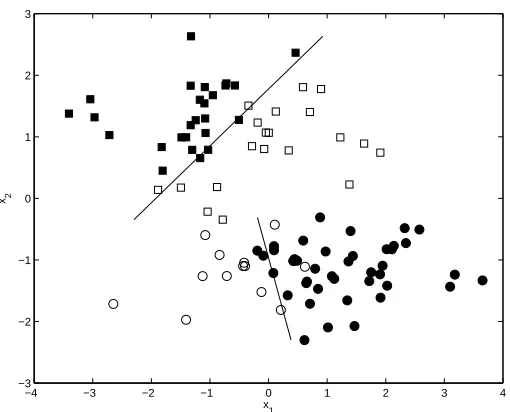
Figure 2: An illustration of our model for a binary (black and white) classification problem with two covariates. Here, the mixture has two components, which are shown with circles and squares. In each component, an MNL model separates the two classes into “black” or “white” with a linear decision boundary. The overall decision boundary, which is a smooth function, is not shown in this figure.
the time of training. For example, the Latent Dirichlet Allocation (LDA) model proposed by Blei et al. (2003) is a well-defined generative model that performs well in classifying documents with previously unknown patterns.
While generative models are quite successful in many problems, they can be computationally in-tensive. Moreover, finding a good (but not perfect) estimate for the joint distribution of all variables (i.e., x and y) does not in general guarantee a good estimate of decision boundaries. By contrast, discriminative models are often computationally fast and are preferred when the covariates are in fact non-random (e.g., they are fixed by an experimental design).
data is provided elsewhere (Shahbaba, 2009), where a Dirichlet process mixture of autoregressive models us used to analyze time-series processes that are subject to regime changes, with no specific economic theory about the structure of the model.
The next section describes our methodology. In Section 3, we illustrate our approach and evalu-ate its performance on simulevalu-ated data. In Section 4, we present the results of applying our model to an actual classification problem, which attempts to identify the folding class of a protein sequence based on the composition of its amino acids. Section 5 discusses another real classification prob-lem, where the objective is to detect Parkinson’s disease. This example is provided to show how our method can be used not only for improving prediction accuracy, but also for identifying hidden structure in the data. Finally, Section 6 is devoted to discussion and future directions.
2. Methodology
We now describe our classification model, which we call dpMNL, in detail. We assume that for each case we observe a vector of continuous covariates, x, of dimension p. The response variable, y, is categorical, with J classes. To model the relationship between y and x, we non-parametrically model the joint distribution of y and x, in the form P(x,y) =P(x)P(y|x), using a Dirichlet process mixture. Within each component of the mixture, the relationship between y and x (i.e., P(y|x)) is expressed using a linear function. The overall relationship becomes nonlinear if the mixture contains more than one component. This way, while we relax the assumption of linearity, the flexibility of the relationship is controlled.
Each component in the mixture model has parameters θ= (µ,σ2,α,β). The distribution of x within a component is multivariate normal, with mean vector µ and diagonal covariance, with the vector σ2 on the diagonal. The distribution of y given x within a component is given by a multinomial logit (MNL) model—for j=1, . . . ,J,
P(y= j|x,α,β) = exp(αj+x
Tβ
j)
∑J
j′=1exp(αj′+xTβj′)
.
The parameterαjis scalar, andβjis a vector of length p. Note that given x, the distribution of y does
not depend on µ andσ. This representation of the MNL model is redundant, since one of theβj’s
(where j=1, ...,J) can be set to zero without changing the set of relationships expressible with the model, but removing this redundancy would make it difficult to specify a prior that treats all classes symmetrically. In this parameterization, what matters is the difference between the parameters of different classes.
In addition to the mixture view, which follows Equation (1) with C→∞, one can also view each
observation, i, as having its own parameter,θi, drawn independently from a distribution drawn from
a Dirichlet process, as in Equation (5):
θi|G ∼ G, for i=1, . . . ,n,
G ∼
D
(G0,γ).Since G will be discrete, many groups of observations will have identical θi, corresponding to
components in the mixture view.
components) dependency is modeled by assigning data to different components (i.e., clustering). The relationship between y and x within a component is captured using an MNL model. Therefore, the relationship is linear locally, but nonlinear globally.
We could assume that y and x are independent within components, and capture the dependence between the response and the covariates by clustering too. However, this may lead to poor per-formance (e.g., when predicting the response for new observations) if the dependence of y on x is difficult to capture using clustering alone. Alternatively, we could also assume that the covariates are dependent within a component. For continuous response variables, this becomes equivalent to the model proposed by M¨uller et al. (1996). If the covariates are in fact dependent, using full co-variance matrices (as suggested by M¨uller et al., 1996) could result in a more parsimonious model since the number of mixture component would be smaller. However, as we discussed above, this approach may be practically infeasible for problems with a moderate to large number of covariates. We believe that our method is an appropriate compromise between these two alternatives.
We define G0, which is a distribution overθ= (µ,σ2,α,β), as follows: µl|µ0,σ0 ∼ N(µ0,σ20),
log(σ2
l)|Mσ,Vσ ∼ N(Mσ,Vσ2),
αj|τ ∼ N(0,τ2),
βjl|ν ∼ N(0,ν2).
The parameters of G0may in turn depend on higher level hyperparameters. For example, we can regard the variances of coefficients as hyperparameters with the following priors:
log(τ2)|Mτ,Vτ ∼ N(Mτ,Vτ2), log(ν2)|Mν,Vν ∼ N(Mν,Vν2).
We use MCMC algorithms for posterior sampling. We could use Gibbs sampling if G0 is the conjugate prior for the likelihood given by F. That is, we would repeatedly draw samples from θi|θ−i,yi (where i=1, ...,n) using the conditional distribution (6). Neal (2000) presented several
algorithms for sampling from the posterior distribution of Dirichlet process mixtures when non-conjugate priors are used. Throughout this paper, we use Gibbs sampling with auxiliary parameters (Neal’s algorithm 8).
This algorithm uses a Markov chain whose state consists of c1, ...,cnandφ= (φc: c∈ {c1, ...,cn}),
so thatθi=φci. In order to allow creation of new clusters, the algorithm temporarily supplements
theφcparameters of existing clusters with m (or m−1) additional parameter values drawn from the
prior, where m a postive integer that can be adjusted to give good performance. Each iteration of the Markov chain simulation operates as follows:
• For i=1, ...,n: Let k−be the number of distinct cjfor j6=i and let h=k−+m. Label these
cjwith values in{1, ...,k−}. If ci=cjfor some j6=i, draw values independently from G0for thoseφcfor which k−<c≤h. If ci=6 cj for all j6=i, let ci have the label k−+1, and draw
values independently from G0 for thoseφc where k−+1<c≤h. Draw a new value for ci
from{1, ...,h}using the following probabilities:
P(ci=c|c−i,yi,φ1, ...,φh) =
b n−i,c
n−1+γF(yi,φc) for 1≤c≤k
−,
b γ/m
n−1+γF(yi,φc) for k
where n−i,cis the number of cjfor j6=i that are equal to c, and b is the appropriate normalizing
constant. Change the state to contain only thoseφc that are now associated with at least to
one observation.
• For all c∈ {c1, ...,cn} draw a new value from the distributionφc | {yi such that ci=c}, or
perform some update that leaves this distribution invariant.
Throughout this paper, we set m=5. This algorithm resembles one proposed by MacEachern and M¨uller (1998), with the difference that the auxiliary parameters exist only temporarily, which avoids an inefficiency in MacEachern and M¨uller’s algorithm.
Samples simulated from the posterior distribution are used to estimate posterior predictive prob-abilities. For a new case with covariates x′, the posterior predictive probability of the response variable, y′, is estimated as follows:
P(y′= j|x′) =P(y
′= j,x′)
P(x′) ,
where
P(y′=j,x′) = 1 S
S
∑
s=1
P(y′= j,x′|G0,θ(s)),
P(x′) = 1 S
S
∑
s=1
P(x′|G0,θ(s)).
Here, S is the number of post-convergence samples from MCMC, and θ(s) represents the set of parameters obtained at iteration s. Alternatively, we could predict new cases using P(y′= j,x′) =
1
S∑
S
s=1P(y′= j|x′,G0,θ(s)). While this would be computationally faster, the above approach allows us to learn from the covariates of test cases when predicting their response values. Note also that the above predictive probabilities include the possibility that the test case is from a new cluster.
We use these posterior predictive probabilities to make predictions for test cases, by assigning each test case to the class with the highest posterior predictive probability. This is the optimal strat-egy for a simple 0/1 loss function. In general, we could use more problem-specific loss functions and modify our prediction strategy accordingly.
Implementations for all our models were coded in MATLAB, and are available online athttp:
//www.ics.uci.edu/˜babaks/codes.
3. Results for Simulated Data
In this section, we illustrate our dpMNL model using synthetic data, and compare it with other models as follows:
• A simple MNL model, fitted by maximum likelihood or Bayesian methods.
• A Bayesian MNL model with quadratic terms (i.e., xlxk, where l =1, ...,p and k=1, ...,p),
referred to as qMNL.
• Support Vector Machines (SVMs) (Vapnik, 1995), implemented with the MATLAB “svm-train” and “svmclassify” functions from the Bioinformatics toolbox. Both a linear SVM (LSVM) and a nonlinear SVM with radial basis function kernel (RBF-SVM) were tried.
When the number of classes in a classification problem was bigger than two, LSVM and RBF-SVM used the all-vs-all scheme as suggested by Allwein et al. (2000), F¨urnkranz (2002), and Hsu and Lin (2002). In this scheme, J2binary classifiers are trained where each classifier separates a pair of classes. The predicted class for each test case is decided by using a majority voting scheme where the class with the highest number of votes among all binary classes wins. For RBF-SVM, the scaling parameter,λ, in the RBF kernel, k(x,x′) =exp(−||x−x′||/2λ), was optimized based on a validation set comprised of 20% of training samples.
The models are compared with respect to their accuracy rate and the F1measure. Accuracy rate is defined as the percentage of the times the correct class is predicted. F1is a common measurement in machine learning defined as:
F1 = 1 J
J
∑
j=1
2Aj
2Aj+Bj+Cj
,
where Aj is the number of cases which are correctly assigned to class j, Bj is the number cases
incorrectly assigned to class j, and Cj is the number of cases which belong to the class j but are
assigned to other classes.
We do two tests. In the first test, we generate data according to the dpMNL model. Our objective is to evaluate the performance of our model when the distribution of data is comprised of multiple components. In the second test, we generate data using a smooth nonlinear function. Our goal is to evaluate the robustness of our model when data actually come from a different model.
3.1 Simulation 1
The first test was on a synthetic four-way classification problem with five covariates. Data are generated according to our dpMNL model, except the number of components was fixed at two. Two hyperparameters defining G0were given the following priors:
log(τ2) ∼ N(0,0.12), log(ν2) ∼ N(0,22).
The prior for component parametersθ= (µ,σ2,α,β)defined by this G 0was µl ∼ N(0,1),
log(σ2l) ∼ N(0,22), αj|τ ∼ N(0,τ2),
βjl|ν ∼ N(0,ν2),
where l=1, ...,5 and j=1, ...,4. We randomly draw parametersθ1andθ2for two components as described from this prior. For each component, we then generate 5000 data points by first drawing xil∼N(µl,σl)and then sampling y using the following MNL model:
P(y= j|x,α,β) = exp(αj+xβj) ∑J
j′=1exp(αj′+xβj′)
Model Accuracy (%) F1(%) Baseline 45.57 (1.47) 15.48 (1.77) MNL (Maximum Likelihood) 77.30 (1.23) 66.65 (1.41)
MNL 78.39 (1.32) 66.52 (1.72)
qMNL 83.60 (0.99) 74.16 (1.30) Tree (Cross Validation) 70.87 (1.40) 55.82 (1.69) LSVM 78.61 (1.17) 67.03 (1.51) RBF-SVM 79.09 (0.99) 63.65 (1.44) dpMNL 89.21 (0.65) 81.00 (1.23)
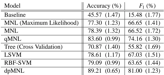
Table 1: Simulation 1: the average performance of models based on 50 simulated data sets. The Baseline model assigns test cases to the class with the highest frequency in the training set. Standard errors of estimates (based on 50 repetitions) are provided in parentheses.
The overall sample size is 10000. We randomly split the data into a training set, with 100 data points, and a test set, with 9900 data points. We use the training set to fit the models, and use the independent test set to evaluate their performance. The regression parameters of the Bayesian MNL model with Bayesian estimation and the qMNL model have the following priors:
αj|τ ∼ N(0,τ2),
βjl|ν ∼ N(0,ν2),
log(τ) ∼ N(0,12), log(ν) ∼ N(0,22).
The above procedure was repeated 50 times. Each time, new hyperparameters,τ2 andν2, and new component parameters,θ1andθ2, were sampled, and a new data set was created based on these θ’s.
We used Hamiltonian dynamics (Neal, 1993) for updating the regression parameters (the α’s andβ’s). For all other parameters, we used single-variable slice sampling (Neal, 2003) with the “stepping out” procedure to find an interval around the current point, and then the “shrinkage” procedure to sample from this interval. We also used slice sampling for updating the concentration parameterγ, We used log(γ)∼N(−3,22)as the prior, which, encourages smaller values ofγ, and hence a smaller number of components. Note that the likelihood for γ depends only on C, the number of unique components (Neal, 2000; Escobar and West, 1995). For all models we ran 5000 MCMC iterations to sample from the posterior distributions. We discarded the initial 500 samples and used the rest for prediction.
0 0.5 1 1.5 2 2.5 3 3.5 4 4.5 5 0
0.5 1 1.5 2 2.5 3 3.5 4 4.5 5
x
1
x2
1 2
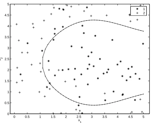
Figure 3: A random sample generated according to Simulation 2, with a3=0. The dotted line is the optimal boundary function.
The average results (over 50 repetitions) are presented in Table 1. As we can see, our dpMNL model provides better results compared to all other models. The improvements are statistically significant (p-values<0.001) for comparisons of accuracy rates using a paired t-test with n=50.
3.2 Simulation 2
In the above simulation, since the data were generated according to the dpMNL model, it is not surprising that this model had the best performance compared to other models. In fact, as we increase the number of components, the amount of improvement using our model becomes more and more substantial (results not shown). To evaluate the robustness of the dpMNL model, we performed another test. This time, we generated xi1,xi2,xi3 (where i=1, ...,10000) from the U ni f orm(0,5)
distribution, and generated a binary response variable, yi, according the following model:
P(y=1|x) = 1
1+exp[a1sin(x11.04+1.2) +x1cos(a2x2+0.7) +a3x3−2] ,
where a1, a2 and a3 are randomly sampled from N(1,0.52). The function used to generate y is a smooth nonlinear function of covariates. The covariates are not clustered, so the generated data do not conform with the assumptions of our model. Moreover, this function includes a completely arbitrary set of constants to ensure the results are generalizable. Figure 3 shows a random sample from this model except that a3is fixed at zero (so x3is ignored). In this figure, the dotted line is the optimal decision boundary.
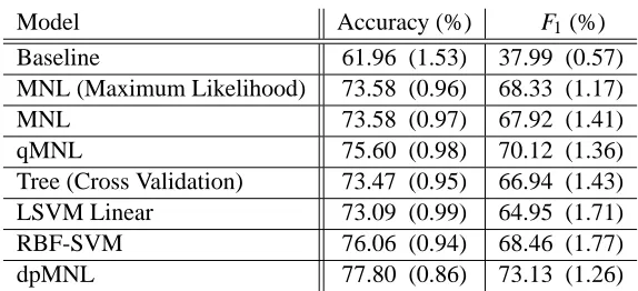
Model Accuracy (%) F1(%) Baseline 61.96 (1.53) 37.99 (0.57) MNL (Maximum Likelihood) 73.58 (0.96) 68.33 (1.17)
MNL 73.58 (0.97) 67.92 (1.41)
qMNL 75.60 (0.98) 70.12 (1.36) Tree (Cross Validation) 73.47 (0.95) 66.94 (1.43) LSVM Linear 73.09 (0.99) 64.95 (1.71) RBF-SVM 76.06 (0.94) 68.46 (1.77) dpMNL 77.80 (0.86) 73.13 (1.26)
Table 2: Simulation 2: the average performance of models based on 50 simulated data sets. The Baseline model assigns test cases to the class with the highest frequency in the training set. Standard errors of estimates (based on 50 repetitions) are provided in parentheses.
(all p-values are smaller than 0.001) better performance compared to all other models. This time, however, the performances of qMNL and RBF-SVM are closer to the performance of the dpMNL model.
4. Results on Real Classification Problems
In this section, we first apply our model the problem of predicting a protein’s 3D structure (i.e., folding class) based on its sequence. We then use our model to identify patients with Parkinson’s disease (PD) based on their speech signals.
4.1 Protein Fold Classification
When predicting a protein’s 3D structure, it is common to presume that the number of possible folds is fixed, and use a classification model to assign a protein to one of these folding classes. There are more than 600 folding patterns identified in the SCOP (Structural Classification of Pro-teins) database (Lo Conte et al., 2000). In this database, proteins are considered to have the same folding class if they have the same major secondary structure in the same arrangement with the same topological connections.
We apply our model to a protein fold recognition data set provided by Ding and Dubchak (2001). The proteins in this data set are obtained from the PDB select database (Hobohm et al., 1992; Hobohm and Sander, 1994) such that two proteins have no more than 35% of the sequence identity for aligned subsequences larger than 80 residues. Originally, the resulting data set included 128 unique folds. However, Ding and Dubchak (2001) selected only the 27 most populated folds (311 proteins) for their analysis. They evaluated their models based on an independent sample (i.e., test set) obtained from PDB-40D (Lo Conte et al., 2000). PDB-40D contains the SCOP sequences with less than 40% identity with each other. Ding and Dubchak (2001) selected 383 representatives of the same 27 folds in the training set with no more than 35% identity to the training sequences. The training and test data sets are available online athttp://crd.lbl.gov/˜cding/protein/.
and Dubchak (2001), who trained several Support Vector Machines (SVM) with nonlinear kernel functions.
We centered the covariates so they have mean zero, and used the following priors for the MNL model and qMNL model (with no interactions, only xi and x2i as covariates):
αj|η ∼ N(0,η2),
log(η2) ∼ N(0,22), βjl|ξ,σl ∼ N(0,ξ2σ2l),
log(ξ2) ∼ N(0,1), log(σ2l) ∼ N(−3,42).
Here, the hyperparameters for the variances of regression parameters are more elaborate than in the previous section. One hyperparameter, σl, is used to control the variance of all coefficients, βjl
(where j=1, ...,J), for covariate xl. If a covariate is irrelevant, its hyperparameter will tend to be
small, forcing the coefficients for that covariate to be near zero. This method, termed Automatic Relevance Determination (ARD), has previously been applied to neural network models by Neal (1996). We also used another hyperparameter,ξ, to control the overall magnitude of allβ’s. This way,σl controls the relevance of covariate xlcompared to other covariates, andξcontrols the overall
usefulness of all covariates in separating all classes. The standard deviation ofβjlis therefore equal
toξσl.
The above scheme was also used for the dpMNL model. Note that in this model, oneσlcontrols
all βjlc, where j=1, ...,J indexes classes, and c=1, ...,C indexes the unique components in the
mixture. Therefore, the standard deviation ofβjlcisξσlνc. Here,νc is specific to each component
c, and controls the overall effect of coefficients in that component. That is, while σ and ξ are global hyperparameters common between all components, νc is a local hyperparameter within a
component. Similarly, the standard deviation of intercepts, αjc in component c isητc. We used
N(0,1)as the prior forνcandτc.
We also needed to specify priors for µl andσl, the mean and standard deviation of covariate xl,
where l=1, ...,p. For these parameters, we used the following priors:
µlc|µ0,l,σ0,l ∼ N(µ0,l,σ20,l),
µ0,l ∼ N(0,52),
log(σ20,l) ∼ N(0,22), log(σ2lc)|Mσ,l,Vσ,l ∼ N(Mσ,l,Vσ2,l),
Mσ,l ∼ N(0,12),
log(Vσ2,l) ∼ N(0,22).
These priors make use of higher level hyperparameters to provide flexibility. For example, if the components are not different with respect to covariate xl, the corresponding variance,σ20,l, becomes
small, forcing µlcclose to their overall mean, µ0,l.
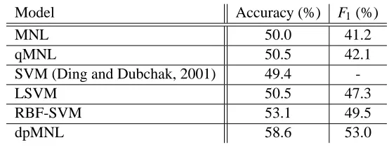
Model Accuracy (%) F1(%)
MNL 50.0 41.2
qMNL 50.5 42.1
SVM (Ding and Dubchak, 2001) 49.4
-LSVM 50.5 47.3
RBF-SVM 53.1 49.5
dpMNL 58.6 53.0
Table 3: Performance of models based on protein fold classification data.
The results for MNL, qMNL, LSVM, RBF-SVM, and dpMNL are presented in Table 3, along with the results for the best SVM model developed by Ding and Dubchak (2001) on the exact same data set. As we can see, the nonlinear RBF-SVM model that we fit has better accuracy than the linear models. Our dpMNL model provides an additional improvement over the RBF-SVM model. This shows that there is in fact a nonlinear relationship between folding classes and the composition of amino acids, and our nonlinear model could successfully identify this relationship.
4.2 Detecting Parkinson’s Disease
The above example shows that our method can potentially improve prediction accuracy, though of course other classifiers, such as SVM and neural networks, may do better on some problems. However, we believe the application of our method is not limited to simply improving prediction accuracy—it can also be used to discover hidden structure in data by identifying subgroups (i.e., mixture components) in the population. This section provides an example to illustrate this concept. Neurological disorders such as Parkinson’s disease (PD) have profound consequences for pa-tients, their families, and society. Although there is no cure for PD at this time, it is possible to alleviate its symptoms significantly, especially at the early stages of the disease (Singh et al., 2007). Since approximately 90% of patients exhibit some form of vocal impairment (Ho et al., 1998), and research has shown that vocal impairment could be one of the earliest indicators of onset of the illness (Duffy, 2005), voice measurement has been proposed as a reliable tool to detect and monitor PD (Sapir et al., 2007; Rahn et al., 2007; Little et al., 2008). For example, patients with PD com-monly display a symptom known as dysphonia, which is an impairment in the normal production of vocal sounds.
In a recent paper, Little et al. (2008) show that by detecting dysphonia, we could identify pa-tients with PD. Their study used data on sustained vowel phonations from 31 subjects, of whom 23 were diagnosed with PD. The 22 covariates used include traditional variables, such as measures of vocal fundamental frequency and measures of variation in amplitude of signals, as well as a novel measurement referred to as pitch period entropy (PPE). See Little et al. (2008) for a detailed de-scription of these variables. This data set is publicly available at UCI Machine Learning Repository
(http://archive.ics.uci.edu/ml/datasets/Parkinsons).
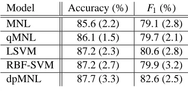
Model Accuracy (%) F1(%) MNL 85.6 (2.2) 79.1 (2.8) qMNL 86.1 (1.5) 79.7 (2.1) LSVM 87.2 (2.3) 80.6 (2.8) RBF-SVM 87.2 (2.7) 79.9 (3.2) dpMNL 87.7 (3.3) 82.6 (2.5)
Table 4: Performance of models based on detecting Parkinson’s disease. Standard errors of esti-mates (based on 5 cross-validation folds) are provided in parentheses.
Group Frequency Age Average Male Proportion 1 107 66 (0.7) 0.86 (0.03) 2 12 72 (1.1) 0.83 (0.11) 3 36 63 (1.8) 0.08 (0.04) 4 40 65 (2.2) 0.40 (0.08) Population 195 66 (0.7) 0.60 (0.03)
Table 5: The age average and male proportion for each cluster (i.e., mixture component) identified by our model. Standard errors of estimates are provided in parentheses.
a 5-fold cross validation scheme instead in order to obtain a more accurate estimate of prediction accuracy rate and avoid inflating model performance due to overfitting. As a result, our models cannot be directly compared to that of Little et al. (2008).
We apply our dpMNL model to the same data set, along with MNL and qMNL (no interactions, only xiand x2i as covariates). Although the observations from the same subject are not independent,
we assume they are, as done by Little et al. (2008). Instead of selecting an optimum subset of fea-tures, we used PCA and chose the first 10 principal components. The MCMC algorithm for MNL, qMNL, and dpMNL ran for 3000 iterations (the first 500 iterations were discarded). Simulating the Markov chain took about 0.7 second per iteration (35 minutes per data set) for dpMNL and 0.1 second per iteration (5 minutes per data set) for MNL using a MATLAB implementation on an UltraSPARC III machine. Training the RBF-SVM model took 38 seconds for each data set.
Using the dpMNL model, the most probable number of components in the posterior is four (note that might change from one iteration to another). Table 4 shows the average and standard errors (based on 5-fold cross validation) of the accuracy rate and the F1measure for MNL, LSVM, RBF-SVM, and dpMNL. (But note that the standard errors assume independence of cross-validation folds, which is not really correct.)
The fourth group also includes more female subjects than male subjects, but the disproportionality is not as high as for the third group.
When identifying Parkinson’s disease by detecting dysphonia, it has been shown that gender has a confounding effect (Cnockaert et al., 2008). By grouping the data into clusters, our model has identified (to some extent) the heterogeneity of subjects due to age and gender, even though these covariates were not available to the model. Moreover, by fitting a separate linear model to each component (i.e., conditioning on mixture identifiers), our model approximates the confounding effect of age and gender. For this example, we could have simply taken the age and gender of subjects from Table 1 in Little et al. (2008) and included them in our model. In many situations, however, not all the relevant factors are measured. This could result in unobservable changes in the structure of data. We discuss this concept in more detail elsewhere (Shahbaba, 2009).
5. Discussion and Future Directions
We introduced a new nonlinear classification model, which uses Dirichlet process mixtures to model the joint distribution of the response variable, y, and the covariates, x, non-parametrically. We com-pared our model to several linear and nonlinear alternative methods using both simulated and real data. We found that when the relationship between y and x is nonlinear, our approach provides sub-stantial improvement over alternative methods. One advantage of this approach is that if the rela-tionship is in fact linear, the model can easily reduce to a linear model by using only one component in the mixture. This way, it avoids overfitting, which is a common challenge in many nonlinear models.
We believe our model can provide more interpretable results. In many real problems, the iden-tified components may correspond to a meaningful segmentation of data. Since the relationship between y and x remains linear in each segment, the results of our model can be expressed as a set of linear patterns for different data segments.
0 1 2 3 4 5 6 7 8 9 10 0.35
0.4 0.45 0.5 0.55 0.6 0.65 0.7 0.75 0.8
λ
Accuracy Rate
−5 −4 −3 −2 −1 0 1 2 3 4 5
0.65 0.7 0.75 0.8 0.85 0.9
µγ
Accuracy Rate (Solid Line)
0 10 20 30 40 50
Number of Component (Dashed Line)
(a) (b)
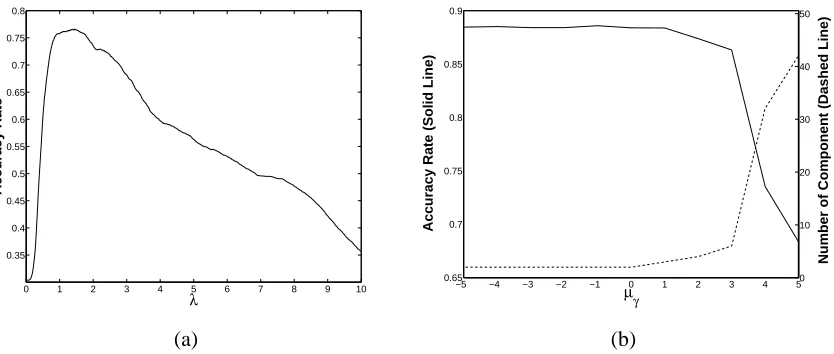
Figure 4: Effects of scale parameters when fitting a data set generated according to Simulation 1. (a) The effect of λ in the RBF-SVM model. (b) The effect of the prior on the scale parameter,γ∼log-N(µγ,22), as µ
γchanges in the dpMNL model.
a substantial decline in accuracy rate (solid line) due to overfitting with a large number of mixture components (dashed line).
The computational cost for our model is substantially higher compared to other methods such as MNL and SVM. This could be a preventive factor in applying our model to some problems. The computational cost of our model could be reduced by using more efficient methods, such as the “split-merge” approach introduced by Jain and Neal (2007). This method uses a Metropolis-Hastings procedure that resamples clusters of observations simultaneously rather than incrementally assigning one observation at a time to mixture components. Alternatively, it might be possible to reduce the computational cost by using a variational inference algorithm similar to the one proposed by Blei and Jordan (2005). In this approach, the posterior distribution P is approximated by a tractable variational distribution Q, whose free variational parameters are adjusted until a reasonable approximation to P is achieved.
We expect our model to outperform other nonlinear models such as neural networks and SVM (with nonlinear kernel functions) when the population is comprised of subgroups each with their own distinct pattern of relationship between covariates and response variable. We also believe that our model could perform well if the true function relating covariates to response variable contains sharp changes.
The performance of our model could be negatively affected if the covariates are highly correlated with each other. In such situations, the assumption of diagonal covariance matrix for x adopted by our model could be very restrictive. To capture the interdependencies between covariates, our model would attempt to increase the number of mixture components (i.e., clusters). This however is not very efficient. To address this issue, we could use mixtures of factor analyzers, where the covariance structure of high dimensional data is model using a small number of latent variables (see for example, Rubin and Thayer, 2007; Ghahramani and Hinton, 1996).
nor-mal distribution in the baseline, G0, with a more appropriate distribution. For example, when the covariate x is binary, we can assume x∼Bernoulli(µ), and specify an appropriate prior distribution (e.g., Beta distribution) for µ. Alternatively, we can use a continuous latent variable, z, such that µ=exp(z)/{1+exp(z)}. This way, we can still model the distribution of z as a mixture of nor-mals. For categorical covariates, we can either use a Dirichlet prior for the probabilities of the K categories, or use K continuous latent variables, z1, ...,zK, and let the probability of category j be
exp(zj)/∑Kj′exp(zj′).
Throughout this paper, we assumed that the relationship between y and x is linear within each component of the mixture. It is possible of course to relax this assumption in order to obtain more flexibility. For example, we can include some nonlinear transformation of the original variables (e.g., quadratic terms) in the model.
Our model can also be extended to problems where the response variable is not multinomial. For example, we can use this approach for regression problems with continuous response, y, which could be assumed normal within a component. We would model the mean of this normal distribution as a linear function of covariates for cases that belong to that component. Other types of response variables (i.e., with Poisson distribution) can be handled in a similar way.
In the protein fold prediction problem discussed in this paper, classes were regarded as a set of unrelated entities. However, these classes are not completely unrelated, and can be grouped into four major structural classes known asα,β,α/β, andα+β. Ding and Dubchak (2001) show the corresponding hierarchical scheme (Table 1 in their paper). We have previously introduced a new approach for modeling hierarchical classes (Shahbaba and Neal, 2006, 2007). In this approach, we use a Bayesian form of the multinomial logit model, called corMNL, with a prior that introduces correlations between the parameters for classes that are nearby in the hierarchy. Our dpMNL model can be extend to classification problems where classes have a hierarchical structure (Shahbaba, 2007). For this purposse, we use a corMNL model, instead of MNL, to capture the relationship between the covariates, x, and the response variable, y, within each component. The results is a nonlinear model which takes the hierarchical structure of classes into account.
Finally, our approach provides a convenient framework for semi-supervised learning, in which both labeled and unlabeled data are used in the learning process. In our approach, unlabeled data can contribute to modeling the distribution of covariates, x, while only labeled data are used to identify the dependence between y and x. This is a quite useful approach for problems where the response variable is known for a limited number of cases, but a large amount of unlabeled data can be generated. One such problem is classification of web documents.
Acknowledgments
This research was supported by the Natural Sciences and Engineering Research Council of Canada. Radford Neal holds a Canada Research Chair in Statistics and Machine Learning.
References
C. E. Antoniak. Mixture of Dirichlet process with applications to Bayesian nonparametric problems. Annals of Statistics, 273(5281):1152–1174, 1974.
D. Blackwell and J. B. MacQueen. Ferguson distributions via polya urn scheme. Annals of Statistics, 1:353–355, 1973.
D. M. Blei and M. I. Jordan. Variational inference for dirichlet process mixtures. Bayesian Analysis, 1:121–144, 2005.
D. M. Blei, A. Y. Ng, and M. I. Jordan. Latent Dirichlet allocation. Journal of Machine Learning Research, 3:993–1022, January 2003.
L. Breiman, J. Friedman, R. A. Olshen, and C. J. Stone. Classification and Regression Trees. Chapman and Hall, Boca Raton, 1993.
C. A. Bush and S. N. MacEachern. A semi-parametric Bayesian model for randomized block designs. Biometrika, 83:275–286, 1996.
B. Cai and D. B. Dunson. Bayesian covariance selection in generalized linear mixed models. Bio-metrics, 62:446–457, 2006.
L. Cnockaert, J. Schoentgen, P. Auzou, C. Ozsancak, L. Defebvre, and F. Grenez. Low-frequency vocal modulations in vowels produced by parkinsonian subjects. Speech Communication, 50(4): 288–300, 2008.
M. J. Daniels and R. E. Kass. Nonconjugate Bayesian estimation of covariance matrices and its use in hierarchical models. Journal of the American Statistical Association, 94(448):1254–1263, 1999.
C. H. Q. Ding and I. Dubchak. Multi-class protein fold recognision using support vector machines and neural networks. Bioinformatics, 17(4):349–358, 2001.
J. R. Duffy. Motor Speech Disorders: Substrates, Differential Diagnosis and Management. Elsevier Mosby, St. Louis, Mo., 2nd edition, 2005.
M. D. Escobar and M. West. Bayesian density estimation and inference using mixtures. Journal of American Statistical Society, 90:577–588, 1995.
T. S. Ferguson. A Bayesian analysis of some nonparametric problems. Annals of Statistics, 1: 209–230, 1973.
T. S. Ferguson. Recent Advances in Statistics, Ed: Rizvi, H. and Rustagi, J., chapter Bayesian density estimation by mixtures of normal distributions, pages 287–302. Academic Press, New York, 1983.
J. F¨urnkranz. Round robin classification. Journal of Machine Learning Research, 2:721–747, 2002. ISSN 1533-7928.
A. K. Ho, R. Iansek, C. Marigliani, J. L. Bradshaw, and S. Gates. Speech impairment in a large sample of patients with Parkinson’s disease. Behavioural Neurology, 11:131–137, 1998.
U. Hobohm and C. Sander. Enlarged representative set of proteins. Protein Science, 3:522–524, 1994.
U. Hobohm, M. Scharf, R. Schneider, and C. Sander. Selection of a representative set of structure from the brookhaven protein bank. Protein Science, 1:409–417, 1992.
C. W. Hsu and C. J. Lin. A comparison of methods for multi-class support vector machines. IEEE Transactions on Neural Networks, 13:415–425, 2002.
R. A. Jacobs, M. I. Jordan, S. J. Nowlan, and G. E. Hinton. Adaptive mixtures of local experts. Neural Computation, 3(1):79–87, 1991.
S. Jain and R. M. Neal. Splitting and merging components of a nonconjugate Dirichlet process mixture model (with discussion). Bayesian Analysis, 2:445–472, 2007.
M. A. Little, P. E. McSharry, E. J. Hunter, J. Spielman, and L. O. Ramig. Suitability of dyspho-nia measurements for telemonitoring of Parkinson’s disease. IEEE Transactions on Biomedical Engineering, (in press), 2008.
L. Lo Conte, B. Ailey, T.J.P Hubbard, S. E. Brenner, A.G. Murzing, and C. Chothia. Scop: a structural classification of protein database. Nucleic Acids Research, 28:257–259, 2000.
S. N. MacEachern and P. M¨uller. Estimating mixture of Dirichlet process models. Journal of Computational and Graphcal Statistics, 7:223–238, 1998.
E. Meeds and S. Osindero. An alternative infinite mixture of Gaussian process experts. Advances in Neural Information Processing Systems, 18:883, 2006.
P. M¨uller, A. Erkanli, and M. West. Bayesian curve fitting using multivariate mormal mixtures. Biometrika, 83(1):67–79, 1996.
R. M. Neal. Markov chain sampling methods for Dirichlet process mixture models. Journal of Computational and Graphical Statistics, 9:249–265, 2000.
R. M. Neal. Slice sampling. Annals of Statistics, 31(3):705–767, 2003.
R. M. Neal. Probabilistic Inference Using Markov Chain Monte Carlo Methods. Technical Report CRG-TR-93-1, Department of Computer Science, University of Toronto, 1993.
R. M. Neal. Bayesian Learning for Neural Networks. Lecture Notes in Statistics No. 118, New York: Springer-Verlag, 1996.
D. A. Rahn, M. Chou, J. J. Jiang, and Y. Zhang. Phonatory impairment in Parkinson’s disease: evidence from nonlinear dynamic analysis and perturbation analysis.(Clinical report). Journal of Voice, 21:64–71, 2007.
D. Rubin and D. Thayer. EM algorithms for ML factor analysis. Pshychometrika, 47(1):69–76, 2007.
S. Sapir, J. L. Spielman, L. O. Ramig, B. H. Story, and C. Fox. Effects of intensive voice treatment (the Lee Silverman Voice Treatment [lsvt]) on vowel articulation in dysarthric individuals with idiopathic Parkinson disease: Acoustic and perceptual findings. Journal of Speech, Language, and Hearing Research, 50(4):899–912, 2007.
B. Shahbaba. Discovering hidden structures using mixture models: Application to nonlinear time series processes. Studies in Nonlinear Dynamics & Econometrics, 13(2):Article 5, 2009.
B. Shahbaba. Improving Classification Models When a Class Hierarchy is Available. PhD thesis, Biostatistics, Public Health Sciences, University of Toronto, 2007.
B. Shahbaba and R. M. Neal. Improving classification when a class hierarchy is available using a hierarchy-based prior. Bayesian Analysis, 2(1):221–238, 2007.
B. Shahbaba and R. M. Neal. Gene function classification using Bayesian models with hierarchy-based priors. BMC Bioinformatics, 7:448, 2006.
N. Singh, V. Pillay, and Y. E. Choonara. Advances in the treatment of Parkinson’s disease. Progress in Neurobiology, 81:29–44, 2007.
I. Ulusoy and C. M. Bishop. Generative versus discriminative methods for object recognition. In CVPR ’05: Proceedings of the 2005 IEEE Computer Society Conference on Computer Vision and Pattern Recognition (CVPR’05) - Volume 2, pages 258–265, Washington, DC, USA, 2005. IEEE Computer Society.
V. N. Vapnik. The Nature of Statistical Learning Theory. Springer-Verlag New York, Inc., New York, NY, USA, 1995. ISBN 0-387-94559-8.