International Journal of Industrial Engineering Computations 6 (2015) 379–390
Contents lists available at GrowingScience
International Journal of Industrial Engineering Computations
homepage: www.GrowingScience.com/ijiec
Process parameter optimization based on principal components analysis during machining of hardened steel
Suryakant B. Chandgudea*, Padmakar J. Pawara and Mudigonda Sadaiahb
aK. K. Wagh Institute of Engineering Education and Research, Nashik-422003, Maharashtra, India. bDr. Babasaheb Ambedkar Technological University, Vidyavihar, Lonere- 402103, Maharashtra, India
C H R O N I C L E A B S T R A C T
Article history:
Received October 14 2014 Received in Revised Format February 10 2015
Accepted February 14 2015 Available online
February 16 2015
The optimum selection of process parameters has played an important role for improving the surface finish, minimizing tool wear, increasing material removal rate and reducing machining time of any machining process. In this paper, optimum parameters while machining AISI D2 hardened steel using solid carbide TiAlN coated end mill has been investigated. For optimization of process parameters along with multiple quality characteristics, principal components analysis method has been adopted in this work. The confirmation experiments have revealed that to improve performance of cutting; principal components analysis method would be a useful tool.
© 2015 Growing Science Ltd. All rights reserved
Keywords:
End milling AISI D2
Principal components analysis
1. Introduction
In the world of machining and especially in manufacturing of mould and die components, machining of hardened steel is a vital area for today’s scientific research. Mould and die manufacturers prefer this material due to retention of its high strength and good wear resistant property at elevated temperatures. But from mould and die manufacturer’s point of view, prime necessity is to reduce machining lead time, improve the quality, and reduce cost of production. For machining of hardened steel, the preferred metal cutting process is end milling. This process is characterised by high metal removal rate, better dimensional accuracy and better surface finish. In practice optimization of every machining process parameter is usually difficult; because it requires simultaneously both machining operation experience and knowledge of mathematical algorithms. The problem of optimization in milling process is complex in nature as multiple objectives and number of constraints has to be considered simultaneously. Moreover, the process planner in practice face problem of optimizing cutting parameters simultaneously for number of mutually conflicting objectives such as machining time, flank wear rate, surface roughness, etc. Considering this fact process parameter optimization in end milling becomes a multi-objective type of problem.
* Corresponding author.
E-mail: [email protected] (S. B. Chandgude)
This paper deals with the application of principal components analysis (PCA) method to study the effect of process parameters simultaneously on the performance characteristics during end milling of AISI D2 steel. The results obtained reveals that the surface finish obtained on AISI D2 hardened steel using the proposed approach is close to surface finish in grinding. This leads to elimination of grinding operation after the end milling operation.
2. Literature review
Traditional and non-traditional methods have been applied by various researchers for optimization of process parameters in milling. Traditional methods such as scatter search (Krishna et al., 2006), sequential quadratic programming (Othmani et al., 2011; Shie, 2006) dynamic programming, and method of feasible directions (Othmani et al., 2011) have been employed to the optimization of milling process. However, these methods tend to obtain a local optimum solution and are not suitable for solving complex multimodal problems. Hence, the researchers are now employing non-traditional methods of optimization for solving this class of problems. It is revealed from the literature that researchers had attempted single objective optimization of milling process parameters to achieve desired effects like surface roughness, production rate, machining time, production cost, tool life, and cutting force. Various methods attempted by the researchers for minimization of surface roughness include genetic algorithm (Brezocnik & Kovacic, 2003; Corso et al., 2012), simulated annealing (Corso et al., 2012), and particle swarm optimization (Prakasvidhisarn et al., 2009). The attempts are also made by researchers to maximize the production rate (or minimize machining time) using genetic algorithm (Aggarwal & Xirouchakis, 2012), simulated annealing (Rao & Pawar, 2010), artificial bee colony (Rao & Pawar, 2010), particle swarm optimization (Rao & Pawar, 2010; Gao et al., 2012), harmony search algorithm (Zarei et al., 2009), cuckoo search algorithm (Yildiz, 2012), and teaching learning based optimization algorithm (Pawar & Rao, 2013). Considering cutting force as an objective, researchers employed particle swarm optimization (Farahnakian et al., 2011), for optimization of milling process parameters. Multi-objective optimization for milling process is attempted by researchers using posteriori approaches namely non-dominated sorting genetic algorithm (NSGA) (Wang et al., 2006) and multi-objective particle swarm optimization (MPSO) (Yang et al., 2011).
Although, these methods are successful to determine global optimal process parameter combinations in milling process; their success mainly depends on the accuracy of the mathematical model, and also these methods provide open ended solutions. Hence, in such cases statistical optimization methods may work better. Few researchers tried optimization of surface roughness as a response using grey relational analysis (Yang et al., 2006) and response surface method (Routara et al., 2009). However, it is observed that multi-objective optimization is mostly attempted by earlier researchers using statistical optimization methods. Using response surface method, Premnath et al. (2012) studied the effect of cutting force on the surface roughness simultaneously. Tool life and surface roughness were optimized simultaneously using grey Taguchi method by (Tsao, 2009). Tosun and Pihtili (2010) applied grey relational analysis optimization technique during face milling of 7075 aluminium alloy. Lu et al. (2009) attempted simultaneous optimization of tool life and production rate in end milling operation. Gopalsamy et al., (2009) considered multi-objective optimization aspects of milling process with surface roughness, tool life and machining time as objectives.
Srithar et al. (2014). An experimental study was conducted by Cho et al. (2014) in-order to investigate the surface hardness enhancement of AISI D2 steel by ion nitriding through atomic attrition. Hullapa et al. (2013) explored the use of Magnetic Barkhausen Noise (MBN) to monitor the transformation of austenite to martensite during cooling to sub-zero temperatures. Oliveira et al. (2010) exhibited production and characterization of boride layers on AISI D2 tool steel by thermochemical boriding treatments performed in borax bath. Experimental investigations for machinability during hard turning of AISI D2 cold work tool steel with conventional and wiper ceramic inserts was conducted by Gaitonde et al. (2009). Response surface methodology (RSM) based mathematical models were developed to analyse the effects of depth of cut and machining time on machinability. The quantitative evolution of the residual stress states in surface layers of an AISI D2 steel treated by low energy high current pulsed electron beam was examined by (Zang et al., 2013) using X-ray diffraction technique.
It is thus revealed from the literature that substantial research has been carried out to investigate optimum cutting parameters in end milling. However, very few researchers have attempted to optimize the cutting process parameters using multi-responses simultaneously using principal components analysis. With this understanding, in this study PCA is applied for simultaneous optimization of three important performance measures of the end milling process, which has not been attempted so far by earlier researchers.
3. Principle component analysis
Initially, this technique has been applied to quantify and identify phenomena in social sciences in which it was difficult to directly measure the phenomenal changes. PCA is useful in reduction of data and interpretation of multi-objective sets of data. Currently PCA is finding wide applications in various scientific fields. In this mainly the focus is on correlation analysis of inter-object using linear combinations for each performance measure. To determine optimal combinations during end milling, the algorithm of principal components analysis is given below:
Step 1: Convert the experimental data in to signal-to-noise ratio:
𝜂𝜂𝑖𝑖𝑖𝑖 =−10𝑙𝑙𝑙𝑙𝑙𝑙 �1𝑛𝑛 � 𝑦𝑦𝑖𝑖𝑖𝑖2 𝑛𝑛
𝑖𝑖=1
�
(1)
Step 2: Normalize the signal-to-noise ratio:
𝑥𝑥𝑖𝑖∗(𝑗𝑗) = 𝑥𝑥𝑖𝑖
(𝑜𝑜)(𝑗𝑗)−min𝑥𝑥
𝑖𝑖(𝑜𝑜)(𝑗𝑗)
max𝑥𝑥𝑖𝑖(𝑜𝑜)(𝑗𝑗)−min𝑥𝑥𝑖𝑖(𝑜𝑜)(𝑗𝑗)
(2)
Step 3: Represent the multi-responses by matrix:
𝑋𝑋=�𝑥𝑥1(1)⋮ ⋯ 𝑥𝑥⋱ 1(𝑛𝑛)⋮ 𝑥𝑥𝑚𝑚(1) ⋯ 𝑥𝑥𝑚𝑚(𝑛𝑛)
� (3)
Step 4: Evaluate the correlation coefficient array:
𝑅𝑅𝑖𝑖𝑗𝑗= 𝐶𝐶𝐶𝐶𝐶𝐶�𝑥𝑥𝜎𝜎 𝑖𝑖 (𝑗𝑗),𝑥𝑥𝑖𝑖 (𝑙𝑙)� 𝑥𝑥𝑖𝑖(𝑗𝑗) ×𝜎𝜎𝑥𝑥𝑖𝑖(𝑙𝑙) ,
𝑗𝑗 = 1,2, … . ,𝑛𝑛, 𝑙𝑙= 1,2, … … ,𝑛𝑛 (4)
where, 𝐶𝐶𝐶𝐶𝐶𝐶(𝑥𝑥𝑖𝑖(𝑗𝑗),𝑥𝑥𝑖𝑖(𝑙𝑙)): the covariance of sequences 𝑥𝑥𝑖𝑖(𝑗𝑗) and 𝑥𝑥𝑖𝑖(𝑙𝑙); 𝜎𝜎𝑥𝑥𝑖𝑖(𝑗𝑗): the standard deviation of sequence 𝑥𝑥𝑖𝑖(𝑗𝑗); 𝜎𝜎𝑥𝑥𝑖𝑖(𝑙𝑙): the standard deviation of sequence 𝑥𝑥𝑖𝑖(𝑙𝑙).
Step 5: Calculate the eigenvalues and eigenvectors:
Step 6: Obtain the principal components:
𝑃𝑃𝑖𝑖𝑘𝑘 = � 𝑥𝑥𝑖𝑖 𝑚𝑚
𝑖𝑖=1
(𝑗𝑗) ×𝐶𝐶𝑖𝑖𝑘𝑘
(6)
Step 7: Calculate the Total Principal Component Index:
𝑃𝑃𝑖𝑖 = � 𝑃𝑃𝑖𝑖𝑘𝑘 𝑚𝑚
𝑘𝑘=1
× 𝑒𝑒(𝑘𝑘) (7)
where, 𝑒𝑒(𝑘𝑘) = 𝑒𝑒𝑖𝑖𝑒𝑒(𝑘𝑘)
∑𝑚𝑚𝑘𝑘=1𝑒𝑒𝑖𝑖𝑒𝑒(𝑘𝑘) (8)
𝑒𝑒𝑒𝑒𝑙𝑙(𝑘𝑘) = kth eigenvalue
Step 8: Generate response table and select the optimum levels of cutting parameters:
Control factor Levels
1 2 3
A 𝑣𝑣���1 𝑣𝑣���2 𝑣𝑣���3
B 𝑓𝑓����𝑧𝑧1 𝑓𝑓����𝑧𝑧2 𝑓𝑓����𝑧𝑧3
C 𝑎𝑎����𝑒𝑒1 𝑎𝑎�����𝑒𝑒2 𝑎𝑎�����𝑒𝑒3
D 𝑎𝑎�����𝑝𝑝1 𝑎𝑎�����𝑝𝑝2 𝑎𝑎�����𝑝𝑝3
𝑣𝑣1
���= (𝑇𝑇𝑃𝑃𝐶𝐶𝐼𝐼)1+ (𝑇𝑇𝑃𝑃𝐶𝐶𝐼𝐼)92+⋯+ (𝑇𝑇𝑃𝑃𝐶𝐶𝐼𝐼)9 (9)
Step 9: Calculate the combined objective function (COF):
𝑊𝑊𝑒𝑒𝑒𝑒𝑙𝑙ℎ𝑡𝑡𝑒𝑒𝑡𝑡 𝑛𝑛𝑙𝑙𝑛𝑛𝑛𝑛𝑎𝑎𝑙𝑙𝑒𝑒𝑛𝑛𝑒𝑒𝑡𝑡
𝑣𝑣𝑎𝑎𝑙𝑙𝑣𝑣𝑒𝑒 𝑓𝑓𝑙𝑙𝑛𝑛 𝑒𝑒𝑎𝑎𝑒𝑒ℎ 𝑛𝑛𝑒𝑒𝑟𝑟𝑟𝑟𝑙𝑙𝑛𝑛𝑟𝑟𝑒𝑒= 𝑤𝑤𝑖𝑖 ×
𝑀𝑀𝑒𝑒𝑎𝑎𝑟𝑟𝑣𝑣𝑛𝑛𝑒𝑒𝑡𝑡 𝑣𝑣𝑎𝑎𝑙𝑙𝑣𝑣𝑒𝑒 𝑙𝑙𝑓𝑓 𝑞𝑞𝑣𝑣𝑎𝑎𝑙𝑙𝑒𝑒𝑡𝑡𝑦𝑦 𝑒𝑒ℎ𝑎𝑎𝑛𝑛𝑎𝑎𝑒𝑒𝑡𝑡𝑒𝑒𝑛𝑛𝑒𝑒𝑟𝑟𝑡𝑡𝑒𝑒𝑒𝑒 𝑒𝑒𝑛𝑛 𝑒𝑒𝑎𝑎𝑒𝑒ℎ 𝑛𝑛𝑣𝑣𝑛𝑛 𝑀𝑀𝑒𝑒𝑛𝑛𝑒𝑒𝑛𝑛𝑣𝑣𝑛𝑛 𝑣𝑣𝑎𝑎𝑙𝑙𝑣𝑣𝑒𝑒 𝑙𝑙𝑓𝑓 𝑞𝑞𝑣𝑣𝑎𝑎𝑙𝑙𝑒𝑒𝑡𝑡𝑦𝑦 𝑒𝑒ℎ𝑎𝑎𝑛𝑛𝑎𝑎𝑒𝑒𝑡𝑡𝑒𝑒𝑛𝑛𝑒𝑒𝑟𝑟𝑡𝑡𝑒𝑒𝑒𝑒 𝑒𝑒𝑛𝑛 𝑡𝑡ℎ𝑒𝑒 𝑡𝑡𝑎𝑎𝑡𝑡𝑎𝑎 𝑟𝑟𝑒𝑒𝑡𝑡
(10)
𝑤𝑤𝑖𝑖 = 𝑤𝑤𝑒𝑒𝑒𝑒𝑙𝑙ℎ𝑡𝑡𝑎𝑎𝑙𝑙𝑒𝑒 𝑎𝑎𝑟𝑟𝑟𝑟𝑒𝑒𝑙𝑙𝑛𝑛𝑒𝑒𝑡𝑡 𝑡𝑡𝑙𝑙 𝑡𝑡ℎ𝑒𝑒 𝑞𝑞𝑣𝑣𝑎𝑎𝑙𝑙𝑒𝑒𝑡𝑡𝑦𝑦 𝑒𝑒ℎ𝑎𝑎𝑛𝑛𝑎𝑎𝑒𝑒𝑡𝑡𝑒𝑒𝑛𝑛𝑒𝑒𝑟𝑟𝑡𝑡𝑒𝑒𝑒𝑒
𝑒𝑒= 1,2, … ,𝑛𝑛 ; and 𝑛𝑛 is the number of quality characteristic
𝐶𝐶𝐶𝐶𝐶𝐶= � 𝑊𝑊𝑒𝑒𝑒𝑒𝑙𝑙ℎ𝑡𝑡𝑒𝑒𝑡𝑡 𝑛𝑛𝑙𝑙𝑛𝑛𝑛𝑛𝑎𝑎𝑙𝑙𝑒𝑒𝑛𝑛𝑒𝑒𝑡𝑡 𝑣𝑣𝑎𝑎𝑙𝑙𝑣𝑣𝑒𝑒 𝑓𝑓𝑙𝑙𝑛𝑛 𝑎𝑎𝑙𝑙𝑙𝑙 𝑛𝑛𝑒𝑒𝑟𝑟𝑟𝑟𝑙𝑙𝑛𝑛𝑟𝑟𝑒𝑒𝑟𝑟 𝑒𝑒𝑛𝑛 𝑒𝑒𝑎𝑎𝑒𝑒ℎ 𝑛𝑛𝑣𝑣𝑛𝑛
Step 10: Perform the statistical analysis of variance (ANOVA).
Step 11: Conduct the confirmation run.
4. Experimental Design
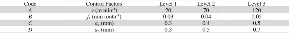
In the present study of end milling, the three quality characteristics selected are machining time, flank wear rate, and surface roughness. These three are directly related to quality of the product and the cost. Control factors and levels have been selected from the machining data handbook (Zhuzhou Co. Ltd., 2011) and are shown in Table 1:
Table 1
Control factors and levels
Code Control Factors Level 1 Level 2 Level 3
A v(m min-1) 20 70 120
B (mm tooth-1)
z
f 0.03 0.04 0.05
C ae(mm) 0.3 0.4 0.5
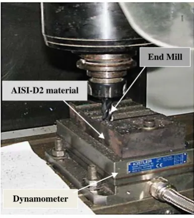
Fig. 1. Experimental set-up: End mill, AISI-D2 hardened steel, and 3-component force dynamometer
The matrix experiments using orthogonal arrays were performed in up-milling mode without any cutting fluid. The factor effects of each level of each control factor can be determined by using the orthogonal arrays. For four factors with three levels L9 array should be used; however, in our study using PCA for multi-objective type of problem, to get into details in the experiment variation, 27 experiments are performed. To eliminate some of the invisible factors that might contribute to the measured variables, each experiment was performed three times in a random sequence. The workpiece was clamped rigidly on dynamometer which is mounted on table of the machine and a fixed overhang length of 25 mm was selected for the tool. The workpiece was continuously cut for a length of 375 mm, with an approach distance and over travel distance of 5 mm, in each pass in order to minimize tool jerks during the physical contact with the workpiece. The complete experimental setup is shown Fig. 1. The cutting time was recorded using the stop watch and tabulated in Table 2. The surface roughness measurements using R-200 series portable surface analyzer was carried at the end of each experiment. The milled surface being anisotropic in nature, the surface roughness measurement was taken at three fixed points; the first point was in the middle and the other two points on the edge of each milled surface. The mean of three surface roughness readings was recorded in Table 2. To observe and measure the maximum flank wear of the end cutting edges, Nikon microscope with a magnification of 100X was used. The flank wear during each experimental run is shown in Fig. 2.
5. Experimental results and discussion
In this section the detail procedure to find optimal combinations of the process parameters using principal components analysis is discussed.
5.1 Optimal Combination of Process Parameters
The results are shown in Table 2. In the experiments, machining time, flank wear, and surface roughness are considered as quality characteristics. These quality characteristics are continuous and nonnegative, and can be recognized as the smallest-the-better type. The results are substituted into Eq. (1) to obtain the S/N ratios of machining time, flank wear rate and surface roughness. Usually, larger the signal-to-noise ratio, better is the quality characteristic. The calculated S/N ratios are normalized using Eq. (2) and are shown in Table 3.
End Mill
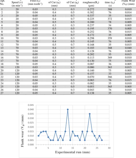
Table 2
Dataset for measured values of the responses
Expt. No. Cutting Speed (v) ) 1 -(m min ) z f Feed ( ) 1 -(mm tooth Radial Depth ) e a of Cut (
(mm)
Axial Depth )
p
a of Cut (
(mm) Surface ) a roughness(R (µm) Machining ) m (t time (s) Flank Wear ) (mm) B (V
1 20 0.03 0.3 0.3 0.272 388 0.010
2 20 0.04 0.4 0.5 0.302 76 0.014
3 20 0.05 0.5 0.7 0.337 35 0.015
4 20 0.03 0.4 0.7 0.225 372 0.015
5 20 0.04 0.5 0.5 0.200 78 0.009
6 20 0.05 0.3 0.3 0.237 34 0.005
7 20 0.03 0.5 0.5 0.195 370 0.005
8 20 0.04 0.3 0.3 0.252 76 0.015
9 20 0.05 0.4 0.7 0.172 35 0.005
10 70 0.03 0.3 0.3 0.298 359 0.010
11 70 0.04 0.4 0.5 0.145 76 0.005
12 70 0.05 0.5 0.7 0.168 35 0.015
13 70 0.03 0.4 0.7 0.103 368 0.040
14 70 0.04 0.5 0.5 0.128 76 0.005
15 70 0.05 0.3 0.3 0.202 35 0.015
16 70 0.03 0.5 0.5 0.113 369 0.010
17 70 0.04 0.3 0.3 0.130 75 0.010
18 70 0.05 0.4 0.7 0.087 36 0.005
19 120 0.03 0.3 0.3 0.080 363 0.015
20 120 0.04 0.4 0.5 0.160 75 0.005
21 120 0.05 0.5 0.7 0.157 33 0.015
22 120 0.03 0.4 0.7 0.070 366 0.035
23 120 0.04 0.5 0.5 0.083 76 0.015
24 120 0.05 0.3 0.3 0.082 35 0.010
25 120 0.03 0.5 0.5 0.053 365 0.005
26 120 0.04 0.3 0.3 0.043 76 0.010
27 120 0.05 0.4 0.7 0.138 35 0.005
Fig. 2. Flank wear during each experimental run
Correlation coefficients are obtained using Eq. (4). From the correlation coefficient array, the eigenvalues and eigenvectors are calculated using MATLAB. From the eigenvalue properties for symmetric matrices, their eigenvectors are always orthogonal to each other. The corresponding eigenvalues (0.7100, 0.9766, and 1.3134) and the eigenvectors (-0.3604, 0.6922, 0.6253), (0.8910, 0.0570, 0.4505), and (0.2762, 0.7194, -0.6373) of the correlation coefficients are obtained using Eq. (5).
0.000 0.005 0.010 0.015 0.020 0.025 0.030 0.035 0.040 0.045
0 5 10 15 20 25 30
Fl a nk w ea r (V B ) (mm)
Table 3
Normalized dataset of Signal-to-Noise ratios
Expt. No. Signal-to-Noise ratio Normalized Signal-to-Noise ratio
a
R tm VB Ra tm VB
1 11.32 -51.777 40.000 0.104 0.000 0.667
2 10.41 -37.616 37.077 0.053 0.657 0.505
3 9.46 -30.881 36.478 0.000 0.970 0.472
4 12.96 -51.411 36.478 0.196 0.017 0.472
5 13.98 -37.786 41.412 0.254 0.650 0.745
6 12.52 -30.630 46.021 0.172 0.982 1.000
7 14.20 -51.352 46.021 0.266 0.020 1.000
8 11.98 -37.559 36.478 0.142 0.660 0.472
9 15.31 -30.881 46.021 0.328 0.970 1.000
10 10.51 -51.102 40.000 0.059 0.031 0.667
11 16.77 -37.559 46.021 0.411 0.660 1.000
12 15.48 -30.881 36.478 0.338 0.970 0.472
13 19.72 -51.305 27.959 0.576 0.022 0.000
14 17.83 -37.559 46.021 0.470 0.660 1.000
15 13.91 -30.756 36.478 0.250 0.976 0.472
16 18.91 -51.329 40.000 0.531 0.021 0.667
17 17.72 -37.501 40.000 0.464 0.663 0.667
18 21.24 -31.005 46.021 0.662 0.964 1.000
19 21.94 -51.198 36.478 0.701 0.027 0.472
20 15.92 -37.501 46.021 0.363 0.663 1.000
21 16.10 -30.238 36.478 0.373 1.000 0.472
22 23.10 -51.258 29.119 0.766 0.024 0.064
23 21.58 -37.616 36.478 0.681 0.657 0.472
24 21.76 -30.881 40.000 0.691 0.970 0.667
25 25.46 -51.234 46.021 0.899 0.025 1.000
26 27.26 -37.559 40.000 1.000 0.660 0.667
27 17.18 -30.881 46.021 0.434 0.970 1.000
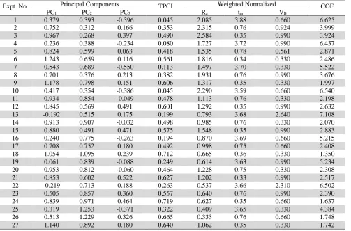
Table 4
Principal components and COF for the experimental runs
Expt. No. Principal Components TPCI Weighted Normalized COF
1
PC PC2 PC3 Ra tm VB
1 0.379 0.393 -0.396 0.045 2.085 3.88 0.660 6.625
2 0.752 0.312 0.166 0.353 2.315 0.76 0.924 3.999
3 0.967 0.268 0.397 0.490 2.584 0.35 0.990 3.924
4 0.236 0.388 -0.234 0.080 1.727 3.72 0.990 6.437
5 0.824 0.599 0.063 0.418 1.535 0.78 0.561 2.871
6 1.243 0.659 0.116 0.561 1.816 0.34 0.330 2.486
7 0.543 0.689 -0.550 0.113 1.497 3.70 0.330 5.522
8 0.701 0.376 0.213 0.382 1.931 0.76 0.990 3.676
9 1.178 0.798 0.151 0.606 1.317 0.35 0.330 1.997
10 0.417 0.354 -0.386 0.045 2.290 3.59 0.660 6.540
11 0.934 0.854 -0.049 0.478 1.113 0.76 0.330 2.198
12 0.845 0.569 0.491 0.601 1.292 0.35 0.990 2.632
13 -0.192 0.515 0.175 0.199 0.793 3.68 2.640 7.108
14 0.913 0.907 -0.032 0.498 0.985 0.76 0.330 2.070
15 0.880 0.491 0.471 0.575 1.548 0.35 0.990 2.883
16 0.240 0.775 -0.263 0.194 0.870 3.69 0.660 5.215
17 0.708 0.752 0.180 0.492 0.998 0.75 0.660 2.408
18 1.054 1.095 0.239 0.712 0.665 0.36 0.330 1.350
19 0.061 0.839 -0.088 0.249 0.614 3.63 0.990 5.234
20 0.953 0.812 -0.060 0.464 1.228 0.75 0.330 2.308
21 0.853 0.602 0.522 0.627 1.202 0.33 0.990 2.517
22 -0.219 0.713 0.188 0.263 0.537 3.66 2.310 6.502
23 0.505 0.857 0.360 0.557 0.640 0.76 0.990 2.390
24 0.839 0.971 0.464 0.719 0.627 0.35 0.660 1.637
25 0.319 1.253 -0.371 0.322 0.409 3.65 0.330 4.384
26 0.513 1.229 0.326 0.665 0.333 0.76 0.660 1.748
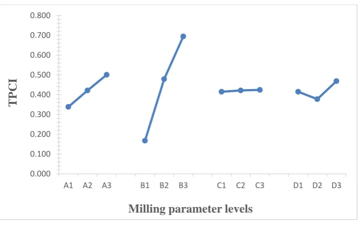
Fig. 3. Response graph of total principal component index (TPCI)
5.2 Obtaining the Principal Components
Principal components analysis is a technique used to transform the correlated variables into linear combinations of uncorrelated variables, which account for most of the variance in the original set of observations. The basic purpose of PCA is to determine the principal components. If the number of linear combinations obtained are n, then the number of principal components formed will be less than or equal to n. With reference to Table 3 and Eq. (6) the principal component (PC1) for experiment 1 can be calculated as follows:
𝑃𝑃𝐶𝐶1 = 0.104 × (−0.3604) + 0 × 0.6922 + 0.667 × 0.6253 = 0.379
The present work deals with three responses and therefore, three principal components PC1, PC2, and PC3 are determined. The corresponding values are included in Table 4.
5.3 Calculating Total Principal Component Index (TPCI)
To obtain best optimal combination of factors/levels, TPCI is calculated using Eq. (7) and Eq. (8). Thus, TPCI for experiment number 1 is calculated as:
(𝑇𝑇𝑃𝑃𝐶𝐶𝐼𝐼)1 = (𝑃𝑃𝐶𝐶1)1 × 0.237 + (𝑃𝑃𝐶𝐶2)1 × 0.326 + (𝑃𝑃𝐶𝐶3)1× 0.438 = 0.045
All the calculated TPCI values are shown in Table 4 accordingly.
5.4 Generate Response Table for Selection of Optimum Parameters
After calculating the TPCI’s for all the experimental run, the next step is to construct the response table. As an illustration in order to calculate the response value for factor A at level 1, using Eq. (9) we get,
𝑣𝑣1
���= (𝑇𝑇𝑃𝑃𝐶𝐶𝐼𝐼)1+ (𝑇𝑇𝑃𝑃𝐶𝐶𝐼𝐼)92+⋯+ (𝑇𝑇𝑃𝑃𝐶𝐶𝐼𝐼)9
𝑣𝑣1
���=0.045 + 0.353 + 0.490 + 0.080 + 0.418 + 0.561 + 0.113 + 0.382 + 0.6069 = 0.3385
0.000 0.100 0.200 0.300 0.400 0.500 0.600 0.700 0.800
A1 A2 A3 B1 B2 B3 C1 C2 C3 D1 D2 D3
TP
CI
Using this method of calculation the remaining response values corresponding to the factors and their respective levels are determined. The maximum value of TPCI corresponding to each factor gives the predicted optimum factor level. Fig. 3 shows response graph of TPCI. From response graph best combination consist of the set: A3 (spindle speed with 120 m min-1), B3 (feed rate with 0.05 mm tooth-1), C3 (radial depth of cut with 0.5 mm), and D3 (axial depth of cut with 0.7 mm).
The combined objective function (COF) for all the quality characteristics is calculated using Eq. (10) by assigning the equal weights of 0.33 for each quality characteristic. Table 4 shows the COF values for all the experimental runs.
5.5 Analysis of Variance
To identify significant factors which influence on performance measures, the ANOVA is carried out for COF and the results are given in Table 5. The significant levels (for α = 0.05, at 95% confidence level) for each source of variation, associated with the F-test are also shown in Table 5. From the principal of
F-test, if F is larger for a specific parameter, the effect on the performance characteristics is greater. In our case from ANOVA table, for feed (factor B), the F value is the largest with a total contribution of 80.61 %; which clearly justifies the major effect on the performance measures such as surface roughness, machining time, and flank wear rate. Cutting speed (factor A) was the second significant factor with 5.00 % contribution. The contribution of radial depth of cut (factor C) was 2.50 %, and the contribution of axial depth of cut was found to be 2. 41 %. The contribution due to error was small and clearly signifies that, important factor has not been omitted and high measurement error was not involved.
Table 5
ANOVA result for Combined Objective Function (COF)
Source Sum of
Squares DOF
Mean
Square F/t P
Contribution
(%) Remark
Model 79.32 7 11.33 24.81 <0.0001 significant
A-v 4.60 2 2.30 5.04 0.0176 5.00
z
f -B
74.03 2 37.02 81.04 <0.0001 80.61
e
a -C
2.30 2 1.15 2.51 0.1075 2.50
p
a -D
2.22 1 2.22 4.86 0.0400 2.41
Residual 8.68 19 0.46 9.45
Cor Total 91.83 26 100
R2 = 0.9014; R2
Adj = 0.8650
5.6 Confirmation Tests
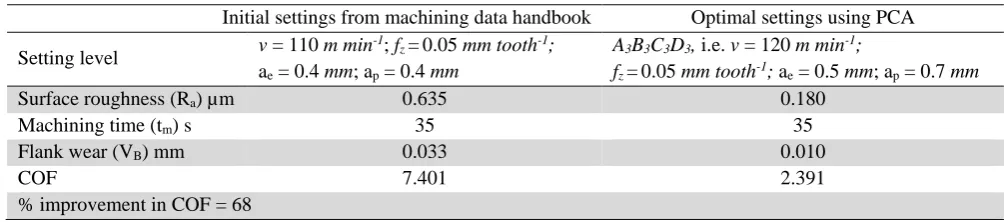
The results of confirmation experiments using the optimal parameters (A3B3C3D3) obtained by PCA with
the initial setting level are shown in Table 6. It has been observed that there is a considerable improvement in the results, due to the application of PCA for optimizing all the three responses simultaneously.
Table 6
Results of initial and optimal settings
Initial settings from machining data handbook Optimal settings using PCA
Setting level v = 110 m min
-1; f
z =0.05 mm tooth-1;
ae = 0.4 mm; ap = 0.4 mm
A3B3C3D3, i.e. v = 120 m min-1;
fz =0.05 mm tooth-1; ae = 0.5 mm; ap = 0.7 mm
Surface roughness (Ra) µm 0.635 0.180
Machining time (tm) s 35 35
Flank wear (VB) mm 0.033 0.010
COF 7.401 2.391
As shown in Table 6, for the problem under consideration, the machining time is constant for the cutting length of 325 mm. The flank wear is decreased from 0.033 mm to 0.010 mm and the surface roughness is decreased from 0.635 µm to 0.180 µm. Through confirmation tests, it is revealed that the results obtained using the proposed approach shows significant improvement over the existing approach.
6. Conclusions
The application of principal components analysis is an approach for optimization of the cutting process parameters during end milling of AISI D2 hardened steel, using 4-flute flattened solid carbide TiAlN coated end mill with straight shank. Based on the results following conclusions can be drawn:
a) The optimal combination (A3B3C3D3) of the cutting parameters using PCA, as shown in Fig. 2 is the
set with; cutting speed (120 m min-1), feed (0.05 mm tooth-1), radial depth of cut (0.5 mm), and axial depth of cut (0.7 mm).
b) The corresponding confirmation test shows 70 % improvement in flank wear rate, and 72 % in surface roughness. The overall improvement considering all three objectives is 68 % over existing parameter setting recommended in the machining data handbook.
c) From this study the surface roughness (Ra) value of 0.180 µm obtained during end milling of AISI
D2 hardened steel material, based on PCA methodology is acceptable to the mould and die manufacturers. Thus, it is likely that it may be possible to eliminate the grinding operation often carried out after end milling operation.
d) The parameters and their levels considered shows highest effect on flank wear (VB) with 43.6 % weightage, 32.6 % weightage for machining time (tm) and 23.7 % weightage for surface roughness (Ra).
e) The results of optimization obtained by the proposed approach provide a ready reference to tool manufacturers as well as to the operators.
It can be concluded that the PCA method is very suitable for solving the flank wear and surface roughness quality problems in milling hardened steel. The cutting forces generated during machining process are important parameters which reflect the machining condition; the cutting forces measured during the experimental run may be helpful in predicting the cutting forces for tool condition monitoring system for future work.
References
Aggarwal, S., & Xirouchakis, P. (2013). Selection of optimal cutting conditions for pocket milling using
genetic algorithm. The International Journal of Advanced Manufacturing Technology, 66(9-12),
1943-1958.
Brezocnik, M., & Kovacic, M. (2003). Integrated genetic programming and genetic algorithm approach to predict surface roughness. Materials and Manufacturing Processes, 18, 475-491.
Cho, K. T., Song, K., Oh, S. H., Lee, Y. K., & Lee, W. B. (2014). Enhanced surface hardening of AISI D2 steel by atomic attrition during Ion Nitriding. 251, 115-121.
Conci, M. P., Bozzi, A. C., & Franco Jr, A. R. (2014). Effect of plasma Nitriding potential on tribological bhaviour of AISI D2 cold-worked tool steel. Wear, 317, 188-193.
Corso, L. L., Zeilmann, R. P., Nicola, G. L., Missell, F. P., & Gomes, H. M. (2013). Using optimization procedures to minimize machining time while maintaining surface quality. The International Journal of Advanced Manufacturing Technology, 65(9-12), 1659-1667.
Gaitonde, V. N., Karnik, S. R., Figueira, L., & Davim, J. P. (2009). Machinability investigations in hard turning of AISI D2 cold work tool steel with conventional and wiper ceramic inserts. International Journal of Refractory Metals and Hard Materials, 27(4), 754-763.
Gao, L., Huang, J., & Li, X. (2012). An effective cellular particle swarm optimization for parameters optimization of a multi-pass milling process. Applied Soft Computing, 12(11), 3490-3499.
Gopalsamy, B. M., Mondal, B., & Ghosh, S. (2009). Optimisation of machining parameters for hard
machining: grey relational theory approach and ANOVA. The International Journal of Advanced
Manufacturing Technology, 45(11-12), 1068-1086.
Hindus, S. J., Kumar, S. H., Arockiyaraj, S. X., Kannan, M. V., & Kuppan, P. (2014). Experimental investigation on laser assisted surface tempering of AISI D2 tool steel. Procedia Engineering, 97, 1489-1495.
Huallpa, E. A., Sanchez, J. C., Padovese, L. R., & Goldenstein, H. (2013). Determining Ms temperature on a AISI D2 cold work tool steel using magnetic barkhausen noise. Journal of Alloys and
Compounds, 577S, S726-S730.
Krishna, A. G., & Rao, K. M. (2006). Optimization of machining parameters for milling machine operations using a scatter search approach. International Journal of Advanced Manufacturing Technology, 31, 219-224.
Lu, H. S., Chang, C. K., Hwang, N. C., & Chung, C. T. (2009). Grey relational analysis coupled with principal component analysis for optimization design of the cutting parameters in high speed end milling. Journal of Materials Process Technology, 209, 3808-3817.
Oliveira, C. K., Casteletti, l. C., Neto, L., Totten, G. E., & Heck, S. C. (2010). Production and characterization of boride layers on AISI D2 tool steel. Vacuum, 84, 792-796.
Othmani, R., Hbaieb, M., & Bouzid, W. (2011). Cutting parameter optimization in NC milling.
International Journal of Advanced Manufacturing Technology, 54, 1023-1032.
Pawar, P. J., & Rao, R. V. (2013). Parameter optimization of machining processes using teaching–
learning-based optimization algorithm. The International Journal of Advanced Manufacturing
Technology, 67(5-8), 995-1006.
Prakasvidhisarn, C., Kunnapapdeelert, S., & Yenradee, P. (2009). Optimal cutting condition determination for desired surface roughness in end milling. International Journal of Advanced
Manufacturing Technology, 41, 440-451.
Premnath, A., Alwarsmy, T., & Rajmohan, T. (2012). Experimental investigation and optimization of process parameters in milling of hybrid metal matrix composites. Materials and Manufacturing Processes, 27, 1035-1044.
Rao, R., & Pawar, P. (2010). Parameter optimization of a multi-pass milling process using non-traditional optimization algorithms. Applied Soft Computing, 10, 445-456.
Routara, B. C., Bandyopadhyay, A., & Sahoo, P. (2009). Roughness modeling and optimization in CNC end milling using response surface method: Effect of workpiece material variation. International
Journal of Advanced Manufacturing Technology.
Shie, J. R. (2006). Optimization of dry machining parameters for high-purity graphite in end milling process by artificial neural networks: A case study. Materials and Manufacturing Processes, 21, 838-845.
Tosun, N., & Pihtili, H. (2010). Grey relational analysis of performance characteristics in MQL millin of 7075 Al Alloy. International Journal of Advanced Manufacturing Technology, 46, 509-515.
Tsao, C. C. (2009). Grey-taguchi method to optimize the milling parameters of Alluminium alloy.
International Journal of Advanced Manufacturing Technology, 45, 41-48.
Wang, Z. G., Wong, Y. S., Rahman, M., & Sun, J. (2006). Multi-objective optimization of high speed milling with parallel genetic simulated annealing. International Journal of Advanced Manufacturing Technology, 31, 209-218.
Yang, W., Guo, Y., & Liao, W. (2011). Multi-objective optimization of multi-pass face milling using particle swarm intelligence. International Journal of Advanced Manufacturing Technology, 56, 429-443.
Yang, Y. K., Shie, J. R., & Huang, C. H. (2006). Optimzation of dry machinig parameters for high purity graphite in end milling process. Materials and Manufacturing Processes, 21, 832-837.
Yildiz, A. R. (2013). Cuckoo search algorithm for the selection of optimal machining parameters in milling operations. The International Journal of Advanced Manufacturing Technology, 64(1-4),
55-61.
Zarei, O., Fesanghary, M., Farshi, B., Saffar, R. J., & Razfar, M. R. (2009). Optimizaton of multi-pass face milling via harmony search algorithm. Journal of Materials Process Technology, 209, 2386-2392.
Zhang, K. M., Zou, J. X., Bolle, B., & Grosdidier, T. (2013). Evolution of residual stress states in surface layers of an AISI D2 steel treated by low energy high current pulsed electron beam. Vacuum, 87, 60-68.