447 Information Technology and Control 2018/3/47
Soft Variable Structure
Control of Linear Systems via
Desired Pole Paths
ITC 3/47
Journal of Information Technology and Control
Vol. 47 / No. 3 / 2018 pp. 447-456
DOI 10.5755/j01.itc.47.3.18805 © Kaunas University of Technology
Soft Variable Structure Control of Linear Systems via
Desired Pole Paths
Received 2017/08/10 Accepted after revision 2018/07/26
http://dx.doi.org/10.5755/j01.itc.47.3.18805
Corresponding author: [email protected]
M. Kaheni, M. Hadad Zarif, A. Akbarzadeh Kalat
Faculty of Electrical Engineering and Robotics, Shahrood University of Technology, Shahrood, Iran; phone: +98 233 239 2204; fax: +98 233 239 2209; e-mails: [email protected], [email protected], [email protected]
M. Sami Fadali
Department of Electrical and Biomedical Engineering, Faculty of Engineering, the University of Nevada, Reno, USA; phone: +1 775 784 6951; fax: +1 775 784 6627; e-mail: [email protected]
In this article, a novel method of soft variable structure control of linear systems, desired pole paths, is pro-posed. The proposed method is helpful to reach a fast response when a continuous control signal and satisfac-tion of some constraints are desired. The method selects a desired path for closed loop poles instead of the exact location of poles, then the pole placement in this path is determined by solving an optimization problem subject to a control signal constraint leading to a suboptimal control structure. The stability of the proposed method is provided based on the multivariable circle criterion and the Kalman-Yakubovich-Popov lemma. A design pa-rameter is also introduced in this paper which can adjust a tradeoff between speed of response and smoothness of the control signal. Simulation of a satellite model shows an improvement in shortening the settling time and softening the control signal compared to published soft variable structure control schemes.
KEYWORDS: Circle criterion, Desired pole paths, Linear control, Nonlinear control, Variable structure control.
1. Introduction
Achieving a fast response while shortening the set-tling time is one of the main objectives in an industrial control process. Time optimal control which achieves
chatter-Information Technology and Control 2018/3/47 448
ing of the control signal reduce actuator service life and increase maintenance cost. Other drawbacks are the high control effort and sensitivity to uncertainties and disturbances. Therefore, researchers have pro-posed methods which have settling time close to time optimal control, a continuous control signal, and re-duced control effort [1, 4, 9-10, 14-16, 23].
Variable structure control (VSC) is a strategy in which the control law varies as a function of the state and switches between k pre-designed controllers [1]. The discontinuous function which selects the desired controller is called the selection function. Sliding mode control [19, 22], high order sliding mode con-trol [4, 9], supervisory concon-trol [2-3], hybrid concon-trol [6-7], etc., are some examples of VSC. In VSC, sud-den changes in the control law lead to high frequen-cy switching, which is not desirable in industrial ap-plications. If the number of pre-designed controllers goes to infinity and the selection function becomes continuous, this disadvantage is eliminated and the method is called soft variable structure control (SVSC). SVSCs can be utilized instead of bang-bang control when both a short settling time and continu-ous control signal are desired. The main methods that have been proposed to date in the literature for SVSC, which improve regulation rate, are divided into three main categories:
1 Soft variable structure control employing an im-plicit Lyapunov function [1]
2 Dynamical soft variable structure control [1, 10, 15-16, 23]
3 Soft variable structure control with variable satu-ration [1, 14]
Huge calculation is an obstacle in online implemen-tation of SVSC employing an implicit Lyapunov func-tion. This control method is also too conservative and rarely allows the capacity of the control signal to be fully exploited to decrease settling time. Dynamical SVSC methods have become more popular recently and their applications in singular [15-16, 23] and frac-tional order systems [10] have been reported in the literature. Although their structure is more suited to continuous time models, the response of the system is highly dependent on a designer-defined control tor. Because no relationship between the control vec-tor and performance is available, good performance is highly dependent on the choice of control vector. SVSC with variable saturation, which is recently
de-veloped with S class functions [14], has strict condi-tions to satisfy the input restriction that may prevent efficient utilization of the control signal. In this arti-cle, a novel method is proposed to improve SVSC and resolve the aforementioned obstacles.
The remainder of this paper is organized as follows. After this introduction in the second section, the problem of restricted control signal systems is de-scribed. In the third section, a feedback approach al-gorithm is proposed. The desired poles path approach is described in Section 4. Simulation results are given in Section 5 and conclusions in Section 6.
2. Problem Description
Consider a single input, single output (SISO) control-lable linear system in the state space with differential equation
be utilized instead of bang-bang control when both a short settling time and continuous control signal are desired. The main methods that have been proposed to date in the literature for SVSC, which improve regulation rate, are divided into three main categories:
1- Soft variable structure control employing an implicit Lyapunov function [1]
2- Dynamical soft variable structure control [1, 10, 15-16, 23]
3- Soft variable structure control with variable saturation [1, 14]
Huge calculation is an obstacle in online implementation of SVSC employing an implicit Lyapunov function. This control method is also too conservative and rarely allows the capacity of the control signal to be fully exploited to decrease settling time. Dynamical SVSC methods have become more popular recently and their applications in singular [15-16, 23] and fractional order systems [10] have been reported in the literature. Although their structure is more suited to continuous time models, the response of the system is highly dependent on a designer-defined control vector. Because no relationship between the control vector and performance is available, good performance is highly dependent on the choice of control vector. SVSC with variable saturation, which is recently developed with S class functions [14], has strict conditions to satisfy the input restriction that may prevent efficient utilization of the control signal. In this article, a novel method is proposed to improve SVSC and resolve the aforementioned obstacles.
The remainder of this paper is organized as follows. After this introduction in the second section, the problem of restricted control signal systems is described. In the third section, a feedback approach algorithm is proposed. The desired poles path approach is described in Section 4. Simulation results are given in Section 5 and conclusions in Section 6.
2. Problem Description
Consider a single input, single output (SISO) controllable linear system in the state space with differential equation 𝐱𝐱𝐱𝐱̇=𝐴𝐴𝐴𝐴𝐱𝐱𝐱𝐱+𝐛𝐛𝐛𝐛𝑢𝑢𝑢𝑢, (1) where𝐱𝐱𝐱𝐱 ∈ ℛ𝑛𝑛𝑛𝑛,𝑢𝑢𝑢𝑢 ∈ ℛ . The control input signal is restricted as
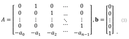
|𝑢𝑢𝑢𝑢|≤ 𝑢𝑢𝑢𝑢0 . (2) Without loss of generality we assume that (1) is in standard controllable form or can be transformed into it. Thus, the state matrix 𝐴𝐴𝐴𝐴and the input matrix 𝐛𝐛𝐛𝐛are in the form
𝐴𝐴𝐴𝐴=
⎣ ⎢ ⎢ ⎢ ⎡ 00
⋮ 0 −𝑎𝑎𝑎𝑎0
1 0 ⋮ 0 −𝑎𝑎𝑎𝑎1
0 1 ⋮ 0 −𝑎𝑎𝑎𝑎2
⋯ … ⋱ ⋯ ⋯
0 0 ⋮ 1 −𝑎𝑎𝑎𝑎𝑛𝑛𝑛𝑛−1⎦
⎥ ⎥ ⎥ ⎤
,𝐛𝐛𝐛𝐛= ⎣ ⎢ ⎢ ⎢ ⎡00
⋮ 0 1⎦⎥
⎥ ⎥ ⎤
. (3)
We require a continuous, fast and stable controller that satisfies the control signal constraint (2), with feasible initial state 𝐱𝐱𝐱𝐱0∈ 𝑋𝑋𝑋𝑋0⊂ ℛ𝑛𝑛𝑛𝑛. Clearly, the requirement of a continuous control signal excludes bang-bang control in this problem.
3. State Feedback Control
Approach
One can choose a state feedback control strategy and endeavor to place the system poles where both stability and the input constraint are met while minimizing settling time. Let us recall some preliminaries.
Theorem 1. Lyapunov Stability [11]
Consider a system with the differential equation, 𝐱𝐱𝐱𝐱̇=𝑓𝑓𝑓𝑓(𝐱𝐱𝐱𝐱), where𝑓𝑓𝑓𝑓(𝐱𝐱𝐱𝐱)is a continuous function with equilibrium point 𝐱𝐱𝐱𝐱= 0. If there exists a function 𝑉𝑉𝑉𝑉(𝐱𝐱𝐱𝐱)with continuous partial derivatives such that:
𝑉𝑉𝑉𝑉(0) = 0
𝑉𝑉𝑉𝑉(𝐱𝐱𝐱𝐱) > 0, 𝐱𝐱𝐱𝐱 ≠0 𝑉𝑉𝑉𝑉̇(𝐱𝐱𝐱𝐱) < 0, 𝐱𝐱𝐱𝐱 ≠0,
then the equilibrium point, 𝐱𝐱𝐱𝐱= 0 , will be asymptotically stable and 𝑉𝑉𝑉𝑉(𝐱𝐱𝐱𝐱) will be called a
Lyapunov function. In linear systems as (1), the
stability theorem is equivalent to finding a positive definite symmetric solution 𝑃𝑃𝑃𝑃 to the Lyapunov equation
𝐴𝐴𝐴𝐴𝑇𝑇𝑇𝑇𝑃𝑃𝑃𝑃+𝑃𝑃𝑃𝑃𝐴𝐴𝐴𝐴=−𝑄𝑄𝑄𝑄 (4) for an arbitrary positive definite matrix, 𝑄𝑄𝑄𝑄. The Lyapunov equation is derived using the quadratic Lyapunov function𝑉𝑉𝑉𝑉(𝐱𝐱𝐱𝐱) =𝐱𝐱𝐱𝐱𝑇𝑇𝑇𝑇𝑃𝑃𝑃𝑃𝐱𝐱𝐱𝐱.
Definition 1.Lyapunov Region [1]
If there exists a function𝑉𝑉𝑉𝑉(𝐱𝐱𝐱𝐱)that satisfies the conditions of Theorem 1 for a system 𝐱𝐱𝐱𝐱̇=𝑓𝑓𝑓𝑓(x)and
𝐺𝐺𝐺𝐺 = {𝐱𝐱𝐱𝐱|𝑉𝑉𝑉𝑉(𝐱𝐱𝐱𝐱) <𝑐𝑐𝑐𝑐} is bounded, then due to
negativity of 𝑉𝑉𝑉𝑉̇(𝐱𝐱𝐱𝐱), 𝐺𝐺𝐺𝐺 is an invariant set and is known as a Lyapunov region.
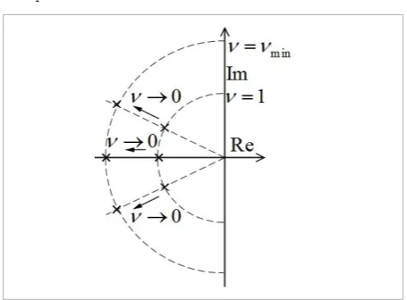
Clearly, placing the closed-loop poles in locations with smaller real values speeds up the response. In this section, we introduce a feedback gain vector function, 𝐤𝐤𝐤𝐤𝑇𝑇𝑇𝑇(𝑣𝑣𝑣𝑣), that places the closed-loop poles on the pole ray depicted in Figure 1 as a function of 𝑣𝑣𝑣𝑣. We define 𝐤𝐤𝐤𝐤𝑇𝑇𝑇𝑇(𝑣𝑣𝑣𝑣)such that
𝑣𝑣𝑣𝑣1<𝑣𝑣𝑣𝑣2⟹
𝑅𝑅𝑅𝑅𝑅𝑅𝑅𝑅 �𝑅𝑅𝑅𝑅𝑒𝑒𝑒𝑒𝑒𝑒𝑒𝑒�𝐴𝐴𝐴𝐴𝑐𝑐𝑐𝑐(𝑣𝑣𝑣𝑣1)��<𝑅𝑅𝑅𝑅𝑅𝑅𝑅𝑅 �𝑅𝑅𝑅𝑅𝑒𝑒𝑒𝑒𝑒𝑒𝑒𝑒�𝐴𝐴𝐴𝐴𝑐𝑐𝑐𝑐(𝑣𝑣𝑣𝑣2)��, where 𝐴𝐴𝐴𝐴𝑐𝑐𝑐𝑐(𝑣𝑣𝑣𝑣) =�𝐴𝐴𝐴𝐴 − 𝐛𝐛𝐛𝐛𝐤𝐤𝐤𝐤𝑇𝑇𝑇𝑇(𝑣𝑣𝑣𝑣)�.
Figure 1 Pole paths (1)
where x∈ℛn, u∈ℛ. The control input signal is restrict-ed as
be utilized instead of bang-bang control when both a short settling time and continuous control signal are desired. The main methods that have been proposed to date in the literature for SVSC, which improve regulation rate, are divided into three main categories:
1- Soft variable structure control employing an implicit Lyapunov function [1]
2- Dynamical soft variable structure control [1, 10, 15-16, 23]
3- Soft variable structure control with variable saturation [1, 14]
Huge calculation is an obstacle in online implementation of SVSC employing an implicit Lyapunov function. This control method is also too conservative and rarely allows the capacity of the control signal to be fully exploited to decrease settling time. Dynamical SVSC methods have become more popular recently and their applications in singular [15-16, 23] and fractional order systems [10] have been reported in the literature. Although their structure is more suited to continuous time models, the response of the system is highly dependent on a designer-defined control vector. Because no relationship between the control vector and performance is available, good performance is highly dependent on the choice of control vector. SVSC with variable saturation, which is recently developed with S class functions [14], has strict conditions to satisfy the input restriction that may prevent efficient utilization of the control signal. In this article, a novel method is proposed to improve SVSC and resolve the aforementioned obstacles.
The remainder of this paper is organized as follows. After this introduction in the second section, the problem of restricted control signal systems is described. In the third section, a feedback approach algorithm is proposed. The desired poles path approach is described in Section 4. Simulation results are given in Section 5 and conclusions in Section 6.
2. Problem Description
Consider a single input, single output (SISO) controllable linear system in the state space with differential equation
𝐱𝐱𝐱𝐱̇=𝐴𝐴𝐴𝐴𝐱𝐱𝐱𝐱+𝐛𝐛𝐛𝐛𝑢𝑢𝑢𝑢, (1) where 𝐱𝐱𝐱𝐱 ∈ ℛ𝑛𝑛𝑛𝑛,𝑢𝑢𝑢𝑢 ∈ ℛ . The control input signal is restricted as
|𝑢𝑢𝑢𝑢|≤ 𝑢𝑢𝑢𝑢0 . (2) Without loss of generality we assume that (1) is in standard controllable form or can be transformed into it. Thus, the state matrix 𝐴𝐴𝐴𝐴and the input matrix 𝐛𝐛𝐛𝐛are in the form
𝐴𝐴𝐴𝐴=
⎣ ⎢ ⎢ ⎢ ⎡ 00
⋮
0
−𝑎𝑎𝑎𝑎0 1 0
⋮
0
−𝑎𝑎𝑎𝑎1 0 1
⋮
0
−𝑎𝑎𝑎𝑎2
⋯
…
⋱ ⋯ ⋯
0 0
⋮
1
−𝑎𝑎𝑎𝑎𝑛𝑛𝑛𝑛−1⎦
⎥ ⎥ ⎥ ⎤
,𝐛𝐛𝐛𝐛=
⎣ ⎢ ⎢ ⎢ ⎡00
⋮
0 1⎦⎥
⎥ ⎥ ⎤
. (3)
We require a continuous, fast and stable controller that satisfies the control signal constraint (2), with feasible initial state 𝐱𝐱𝐱𝐱0∈ 𝑋𝑋𝑋𝑋0⊂ ℛ𝑛𝑛𝑛𝑛. Clearly, the requirement of a continuous control signal excludes bang-bang control in this problem.
3. State Feedback Control
Approach
One can choose a state feedback control strategy and endeavor to place the system poles where both stability and the input constraint are met while minimizing settling time. Let us recall some preliminaries.
Theorem 1. Lyapunov Stability [11]
Consider a system with the differential equation,
𝐱𝐱𝐱𝐱̇=𝑓𝑓𝑓𝑓(𝐱𝐱𝐱𝐱), where𝑓𝑓𝑓𝑓(𝐱𝐱𝐱𝐱)is a continuous function with equilibrium point 𝐱𝐱𝐱𝐱= 0. If there exists a function
𝑉𝑉𝑉𝑉(𝐱𝐱𝐱𝐱)with continuous partial derivatives such that:
𝑉𝑉𝑉𝑉(0) = 0
𝑉𝑉𝑉𝑉(𝐱𝐱𝐱𝐱) > 0, 𝐱𝐱𝐱𝐱 ≠0
𝑉𝑉𝑉𝑉̇(𝐱𝐱𝐱𝐱) < 0, 𝐱𝐱𝐱𝐱 ≠0,
then the equilibrium point, 𝐱𝐱𝐱𝐱= 0 , will be asymptotically stable and 𝑉𝑉𝑉𝑉(𝐱𝐱𝐱𝐱) will be called a
Lyapunov function. In linear systems as (1), the
stability theorem is equivalent to finding a positive definite symmetric solution 𝑃𝑃𝑃𝑃 to the Lyapunov equation
𝐴𝐴𝐴𝐴𝑇𝑇𝑇𝑇𝑃𝑃𝑃𝑃+𝑃𝑃𝑃𝑃𝐴𝐴𝐴𝐴=−𝑄𝑄𝑄𝑄 (4) for an arbitrary positive definite matrix, 𝑄𝑄𝑄𝑄. The Lyapunov equation is derived using the quadratic Lyapunov function𝑉𝑉𝑉𝑉(𝐱𝐱𝐱𝐱) =𝐱𝐱𝐱𝐱𝑇𝑇𝑇𝑇𝑃𝑃𝑃𝑃𝐱𝐱𝐱𝐱.
Definition 1.Lyapunov Region [1]
If there exists a function𝑉𝑉𝑉𝑉(𝐱𝐱𝐱𝐱)that satisfies the conditions of Theorem 1 for a system 𝐱𝐱𝐱𝐱̇=𝑓𝑓𝑓𝑓(x)and
𝐺𝐺𝐺𝐺= {𝐱𝐱𝐱𝐱|𝑉𝑉𝑉𝑉(𝐱𝐱𝐱𝐱) <𝑐𝑐𝑐𝑐} is bounded, then due to
negativity of 𝑉𝑉𝑉𝑉̇(𝐱𝐱𝐱𝐱),𝐺𝐺𝐺𝐺 is an invariant set and is known as a Lyapunov region.
Clearly, placing the closed-loop poles in locations with smaller real values speeds up the response. In this section, we introduce a feedback gain vector function, 𝐤𝐤𝐤𝐤𝑇𝑇𝑇𝑇(𝑣𝑣𝑣𝑣), that places the closed-loop poles on the pole ray depicted in Figure 1 as a function of
𝑣𝑣𝑣𝑣. We define 𝐤𝐤𝐤𝐤𝑇𝑇𝑇𝑇(𝑣𝑣𝑣𝑣)such that
𝑣𝑣𝑣𝑣1<𝑣𝑣𝑣𝑣2⟹
𝑅𝑅𝑅𝑅𝑅𝑅𝑅𝑅 �𝑅𝑅𝑅𝑅𝑒𝑒𝑒𝑒𝑒𝑒𝑒𝑒�𝐴𝐴𝐴𝐴𝑐𝑐𝑐𝑐(𝑣𝑣𝑣𝑣1)��<𝑅𝑅𝑅𝑅𝑅𝑅𝑅𝑅 �𝑅𝑅𝑅𝑅𝑒𝑒𝑒𝑒𝑒𝑒𝑒𝑒�𝐴𝐴𝐴𝐴𝑐𝑐𝑐𝑐(𝑣𝑣𝑣𝑣2)��, where 𝐴𝐴𝐴𝐴𝑐𝑐𝑐𝑐(𝑣𝑣𝑣𝑣) =�𝐴𝐴𝐴𝐴 − 𝐛𝐛𝐛𝐛𝐤𝐤𝐤𝐤𝑇𝑇𝑇𝑇(𝑣𝑣𝑣𝑣)�.
Figure 1 Pole paths (2)
Without loss of generality we assume that (1) is in standard controllable form or can be transformed into it. Thus, the state matrix A and the input matrix b are in the form
be utilized instead of bang-bang control when both a short settling time and continuous control signal are desired. The main methods that have been proposed to date in the literature for SVSC, which improve regulation rate, are divided into three main categories:
1- Soft variable structure control employing an implicit Lyapunov function [1]
2- Dynamical soft variable structure control [1, 10, 15-16, 23]
3- Soft variable structure control with variable saturation [1, 14]
Huge calculation is an obstacle in online implementation of SVSC employing an implicit Lyapunov function. This control method is also too conservative and rarely allows the capacity of the control signal to be fully exploited to decrease settling time. Dynamical SVSC methods have become more popular recently and their applications in singular [15-16, 23] and fractional order systems [10] have been reported in the literature. Although their structure is more suited to continuous time models, the response of the system is highly dependent on a designer-defined control vector. Because no relationship between the control vector and performance is available, good performance is highly dependent on the choice of control vector. SVSC with variable saturation, which is recently developed with S class functions [14], has strict conditions to satisfy the input restriction that may prevent efficient utilization of the control signal. In this article, a novel method is proposed to improve SVSC and resolve the aforementioned obstacles.
The remainder of this paper is organized as follows. After this introduction in the second section, the problem of restricted control signal systems is described. In the third section, a feedback approach algorithm is proposed. The desired poles path approach is described in Section 4. Simulation results are given in Section 5 and conclusions in Section 6.
2. Problem Description
Consider a single input, single output (SISO) controllable linear system in the state space with differential equation
𝐱𝐱𝐱𝐱̇=𝐴𝐴𝐴𝐴𝐱𝐱𝐱𝐱+𝐛𝐛𝐛𝐛𝑢𝑢𝑢𝑢, (1) where 𝐱𝐱𝐱𝐱 ∈ ℛ𝑛𝑛𝑛𝑛,𝑢𝑢𝑢𝑢 ∈ ℛ . The control input signal is restricted as
|𝑢𝑢𝑢𝑢|≤ 𝑢𝑢𝑢𝑢0 . (2) Without loss of generality we assume that (1) is in standard controllable form or can be transformed into it. Thus, the state matrix 𝐴𝐴𝐴𝐴and the input matrix 𝐛𝐛𝐛𝐛are in the form
𝐴𝐴𝐴𝐴=
⎣ ⎢ ⎢ ⎢ ⎡ 00
⋮
0
−𝑎𝑎𝑎𝑎0 1 0
⋮
0
−𝑎𝑎𝑎𝑎1 0 1
⋮
0
−𝑎𝑎𝑎𝑎2
⋯
…
⋱ ⋯ ⋯
0 0
⋮
1
−𝑎𝑎𝑎𝑎𝑛𝑛𝑛𝑛−1⎦
⎥ ⎥ ⎥ ⎤
,𝐛𝐛𝐛𝐛=
⎣ ⎢ ⎢ ⎢ ⎡00
⋮
0 1⎦⎥
⎥ ⎥ ⎤
. (3)
We require a continuous, fast and stable controller that satisfies the control signal constraint (2), with feasible initial state 𝐱𝐱𝐱𝐱0∈ 𝑋𝑋𝑋𝑋0⊂ ℛ𝑛𝑛𝑛𝑛. Clearly, the requirement of a continuous control signal excludes bang-bang control in this problem.
3. State Feedback Control
Approach
One can choose a state feedback control strategy and endeavor to place the system poles where both stability and the input constraint are met while minimizing settling time. Let us recall some preliminaries.
Theorem 1. Lyapunov Stability [11]
Consider a system with the differential equation,
𝐱𝐱𝐱𝐱̇=𝑓𝑓𝑓𝑓(𝐱𝐱𝐱𝐱), where𝑓𝑓𝑓𝑓(𝐱𝐱𝐱𝐱)is a continuous function with equilibrium point 𝐱𝐱𝐱𝐱= 0. If there exists a function
𝑉𝑉𝑉𝑉(𝐱𝐱𝐱𝐱)with continuous partial derivatives such that:
𝑉𝑉𝑉𝑉(0) = 0
𝑉𝑉𝑉𝑉(𝐱𝐱𝐱𝐱) > 0, 𝐱𝐱𝐱𝐱 ≠0
𝑉𝑉𝑉𝑉̇(𝐱𝐱𝐱𝐱) < 0, 𝐱𝐱𝐱𝐱 ≠0,
then the equilibrium point, 𝐱𝐱𝐱𝐱= 0 , will be asymptotically stable and 𝑉𝑉𝑉𝑉(𝐱𝐱𝐱𝐱) will be called a
Lyapunov function. In linear systems as (1), the
stability theorem is equivalent to finding a positive definite symmetric solution 𝑃𝑃𝑃𝑃 to the Lyapunov equation
𝐴𝐴𝐴𝐴𝑇𝑇𝑇𝑇𝑃𝑃𝑃𝑃+𝑃𝑃𝑃𝑃𝐴𝐴𝐴𝐴=−𝑄𝑄𝑄𝑄 (4) for an arbitrary positive definite matrix, 𝑄𝑄𝑄𝑄. The Lyapunov equation is derived using the quadratic Lyapunov function𝑉𝑉𝑉𝑉(𝐱𝐱𝐱𝐱) =𝐱𝐱𝐱𝐱𝑇𝑇𝑇𝑇𝑃𝑃𝑃𝑃𝐱𝐱𝐱𝐱.
Definition 1.Lyapunov Region [1]
If there exists a function𝑉𝑉𝑉𝑉(𝐱𝐱𝐱𝐱)that satisfies the conditions of Theorem 1 for a system 𝐱𝐱𝐱𝐱̇=𝑓𝑓𝑓𝑓(x)and
𝐺𝐺𝐺𝐺= {𝐱𝐱𝐱𝐱|𝑉𝑉𝑉𝑉(𝐱𝐱𝐱𝐱) <𝑐𝑐𝑐𝑐} is bounded, then due to
negativity of 𝑉𝑉𝑉𝑉̇(𝐱𝐱𝐱𝐱), 𝐺𝐺𝐺𝐺 is an invariant set and is known as a Lyapunov region.
Clearly, placing the closed-loop poles in locations with smaller real values speeds up the response. In this section, we introduce a feedback gain vector function, 𝐤𝐤𝐤𝐤𝑇𝑇𝑇𝑇(𝑣𝑣𝑣𝑣), that places the closed-loop poles on the pole ray depicted in Figure 1 as a function of
𝑣𝑣𝑣𝑣. We define 𝐤𝐤𝐤𝐤𝑇𝑇𝑇𝑇(𝑣𝑣𝑣𝑣)such that
𝑣𝑣𝑣𝑣1<𝑣𝑣𝑣𝑣2⟹
𝑅𝑅𝑅𝑅𝑅𝑅𝑅𝑅 �𝑅𝑅𝑅𝑅𝑒𝑒𝑒𝑒𝑒𝑒𝑒𝑒�𝐴𝐴𝐴𝐴𝑐𝑐𝑐𝑐(𝑣𝑣𝑣𝑣1)��<𝑅𝑅𝑅𝑅𝑅𝑅𝑅𝑅 �𝑅𝑅𝑅𝑅𝑒𝑒𝑒𝑒𝑒𝑒𝑒𝑒�𝐴𝐴𝐴𝐴𝑐𝑐𝑐𝑐(𝑣𝑣𝑣𝑣2)��, where 𝐴𝐴𝐴𝐴𝑐𝑐𝑐𝑐(𝑣𝑣𝑣𝑣) =�𝐴𝐴𝐴𝐴 − 𝐛𝐛𝐛𝐛𝐤𝐤𝐤𝐤𝑇𝑇𝑇𝑇(𝑣𝑣𝑣𝑣)�.
Figure 1 Pole paths
(3)
We require a continuous, fast and stable controller that satisfies the control signal constraint (2), with feasible initial state x0 ∈ X0 ⊂ ℛn. Clearly, the require-ment of a continuous control signal excludes bang-bang control in this problem.
449 Information Technology and Control 2018/3/47
settling time. Let us recall some preliminaries. Theorem 1.Lyapunov Stability [11]
Consider a system with the differential equation, x.= f(x), where f(x) is a continuous function with equilib-rium point x= 0. If there exists a function V(x) with continuous partial derivatives such that:
be utilized instead of bang-bang control when both a short settling time and continuous control signal are desired. The main methods that have been proposed to date in the literature for SVSC, which improve regulation rate, are divided into three main categories:
1- Soft variable structure control employing an implicit Lyapunov function [1]
2- Dynamical soft variable structure control [1, 10, 15-16, 23]
3- Soft variable structure control with variable saturation [1, 14]
Huge calculation is an obstacle in online implementation of SVSC employing an implicit Lyapunov function. This control method is also too conservative and rarely allows the capacity of the control signal to be fully exploited to decrease settling time. Dynamical SVSC methods have become more popular recently and their applications in singular [15-16, 23] and fractional order systems [10] have been reported in the literature. Although their structure is more suited to continuous time models, the response of the system is highly dependent on a designer-defined control vector. Because no relationship between the control vector and performance is available, good performance is highly dependent on the choice of control vector. SVSC with variable saturation, which is recently developed with S class functions [14], has strict conditions to satisfy the input restriction that may prevent efficient utilization of the control signal. In this article, a novel method is proposed to improve SVSC and resolve the aforementioned obstacles.
The remainder of this paper is organized as follows. After this introduction in the second section, the problem of restricted control signal systems is described. In the third section, a feedback approach algorithm is proposed. The desired poles path approach is described in Section 4. Simulation results are given in Section 5 and conclusions in Section 6.
2. Problem Description
Consider a single input, single output (SISO) controllable linear system in the state space with differential equation
𝐱𝐱𝐱𝐱̇=𝐴𝐴𝐴𝐴𝐱𝐱𝐱𝐱+𝐛𝐛𝐛𝐛𝑢𝑢𝑢𝑢, (1) where 𝐱𝐱𝐱𝐱 ∈ ℛ𝑛𝑛𝑛𝑛,𝑢𝑢𝑢𝑢 ∈ ℛ . The control input signal is restricted as
|𝑢𝑢𝑢𝑢|≤ 𝑢𝑢𝑢𝑢0 . (2) Without loss of generality we assume that (1) is in standard controllable form or can be transformed into it. Thus, the state matrix 𝐴𝐴𝐴𝐴and the input matrix 𝐛𝐛𝐛𝐛are in the form 𝐴𝐴𝐴𝐴= ⎣ ⎢ ⎢ ⎢ ⎡ 00
⋮ 0 −𝑎𝑎𝑎𝑎0 1 0 ⋮ 0 −𝑎𝑎𝑎𝑎1 0 1 ⋮ 0 −𝑎𝑎𝑎𝑎2 ⋯ … ⋱ ⋯ ⋯ 0 0 ⋮ 1 −𝑎𝑎𝑎𝑎𝑛𝑛𝑛𝑛−1⎦⎥ ⎥ ⎥ ⎤ ,𝐛𝐛𝐛𝐛= ⎣ ⎢ ⎢ ⎢ ⎡00
⋮ 0 1⎦⎥
⎥ ⎥ ⎤
. (3)
We require a continuous, fast and stable controller that satisfies the control signal constraint (2), with feasible initial state 𝐱𝐱𝐱𝐱0∈ 𝑋𝑋𝑋𝑋0⊂ ℛ𝑛𝑛𝑛𝑛. Clearly, the requirement of a continuous control signal excludes bang-bang control in this problem.
3. State Feedback Control
Approach
One can choose a state feedback control strategy and endeavor to place the system poles where both stability and the input constraint are met while minimizing settling time. Let us recall some preliminaries.
Theorem 1. Lyapunov Stability [11]
Consider a system with the differential equation,
𝐱𝐱𝐱𝐱̇=𝑓𝑓𝑓𝑓(𝐱𝐱𝐱𝐱), where𝑓𝑓𝑓𝑓(𝐱𝐱𝐱𝐱)is a continuous function with
equilibrium point 𝐱𝐱𝐱𝐱= 0. If there exists a function
𝑉𝑉𝑉𝑉(𝐱𝐱𝐱𝐱)with continuous partial derivatives such that:
𝑉𝑉𝑉𝑉(0) = 0
𝑉𝑉𝑉𝑉(𝐱𝐱𝐱𝐱) > 0, 𝐱𝐱𝐱𝐱 ≠0
𝑉𝑉𝑉𝑉̇(𝐱𝐱𝐱𝐱) < 0, 𝐱𝐱𝐱𝐱 ≠0,
then the equilibrium point, 𝐱𝐱𝐱𝐱= 0 , will be asymptotically stable and 𝑉𝑉𝑉𝑉(𝐱𝐱𝐱𝐱) will be called a
Lyapunov function. In linear systems as (1), the
stability theorem is equivalent to finding a positive definite symmetric solution 𝑃𝑃𝑃𝑃 to the Lyapunov equation
𝐴𝐴𝐴𝐴𝑇𝑇𝑇𝑇𝑃𝑃𝑃𝑃+𝑃𝑃𝑃𝑃𝐴𝐴𝐴𝐴=−𝑄𝑄𝑄𝑄 (4) for an arbitrary positive definite matrix, 𝑄𝑄𝑄𝑄. The Lyapunov equation is derived using the quadratic Lyapunov function𝑉𝑉𝑉𝑉(𝐱𝐱𝐱𝐱) =𝐱𝐱𝐱𝐱𝑇𝑇𝑇𝑇𝑃𝑃𝑃𝑃𝐱𝐱𝐱𝐱.
Definition 1.Lyapunov Region [1]
If there exists a function𝑉𝑉𝑉𝑉(𝐱𝐱𝐱𝐱)that satisfies the conditions of Theorem 1 for a system 𝐱𝐱𝐱𝐱̇=𝑓𝑓𝑓𝑓(x)and
𝐺𝐺𝐺𝐺= {𝐱𝐱𝐱𝐱|𝑉𝑉𝑉𝑉(𝐱𝐱𝐱𝐱) <𝑐𝑐𝑐𝑐} is bounded, then due to
negativity of 𝑉𝑉𝑉𝑉̇(𝐱𝐱𝐱𝐱),𝐺𝐺𝐺𝐺 is an invariant set and is known as a Lyapunov region.
Clearly, placing the closed-loop poles in locations with smaller real values speeds up the response. In this section, we introduce a feedback gain vector function, 𝐤𝐤𝐤𝐤𝑇𝑇𝑇𝑇(𝑣𝑣𝑣𝑣), that places the closed-loop poles on the pole ray depicted in Figure 1 as a function of 𝑣𝑣𝑣𝑣. We define 𝐤𝐤𝐤𝐤𝑇𝑇𝑇𝑇(𝑣𝑣𝑣𝑣)such that
𝑣𝑣𝑣𝑣1<𝑣𝑣𝑣𝑣2⟹
𝑅𝑅𝑅𝑅𝑅𝑅𝑅𝑅 �𝑅𝑅𝑅𝑅𝑒𝑒𝑒𝑒𝑒𝑒𝑒𝑒�𝐴𝐴𝐴𝐴𝑐𝑐𝑐𝑐(𝑣𝑣𝑣𝑣1)��<𝑅𝑅𝑅𝑅𝑅𝑅𝑅𝑅 �𝑅𝑅𝑅𝑅𝑒𝑒𝑒𝑒𝑒𝑒𝑒𝑒�𝐴𝐴𝐴𝐴𝑐𝑐𝑐𝑐(𝑣𝑣𝑣𝑣2)��, where 𝐴𝐴𝐴𝐴𝑐𝑐𝑐𝑐(𝑣𝑣𝑣𝑣) =�𝐴𝐴𝐴𝐴 − 𝐛𝐛𝐛𝐛𝐤𝐤𝐤𝐤𝑇𝑇𝑇𝑇(𝑣𝑣𝑣𝑣)�.
Figure 1 Pole paths
then the equilibrium point, x= 0, will be asymptoti-cally stable and V(x) will be called a Lyapunov func-tion. In linear systems as (1), the stability theorem is equivalent to finding a positive definite symmetric solution P to the Lyapunov equation
be utilized instead of bang-bang control when both a short settling time and continuous control signal are desired. The main methods that have been proposed to date in the literature for SVSC, which improve regulation rate, are divided into three main categories:
1- Soft variable structure control employing an implicit Lyapunov function [1]
2- Dynamical soft variable structure control [1, 10, 15-16, 23]
3- Soft variable structure control with variable saturation [1, 14]
Huge calculation is an obstacle in online implementation of SVSC employing an implicit Lyapunov function. This control method is also too conservative and rarely allows the capacity of the control signal to be fully exploited to decrease settling time. Dynamical SVSC methods have become more popular recently and their applications in singular [15-16, 23] and fractional order systems [10] have been reported in the literature. Although their structure is more suited to continuous time models, the response of the system is highly dependent on a designer-defined control vector. Because no relationship between the control vector and performance is available, good performance is highly dependent on the choice of control vector. SVSC with variable saturation, which is recently developed with S class functions [14], has strict conditions to satisfy the input restriction that may prevent efficient utilization of the control signal. In this article, a novel method is proposed to improve SVSC and resolve the aforementioned obstacles.
The remainder of this paper is organized as follows. After this introduction in the second section, the problem of restricted control signal systems is described. In the third section, a feedback approach algorithm is proposed. The desired poles path approach is described in Section 4. Simulation results are given in Section 5 and conclusions in Section 6.
2. Problem Description
Consider a single input, single output (SISO) controllable linear system in the state space with differential equation
𝐱𝐱𝐱𝐱̇=𝐴𝐴𝐴𝐴𝐱𝐱𝐱𝐱+𝐛𝐛𝐛𝐛𝑢𝑢𝑢𝑢, (1) where 𝐱𝐱𝐱𝐱 ∈ ℛ𝑛𝑛𝑛𝑛,𝑢𝑢𝑢𝑢 ∈ ℛ . The control input signal is restricted as
|𝑢𝑢𝑢𝑢|≤ 𝑢𝑢𝑢𝑢0 . (2) Without loss of generality we assume that (1) is in standard controllable form or can be transformed into it. Thus, the state matrix 𝐴𝐴𝐴𝐴and the input matrix 𝐛𝐛𝐛𝐛are in the form 𝐴𝐴𝐴𝐴= ⎣ ⎢ ⎢ ⎢ ⎡ 00
⋮ 0 −𝑎𝑎𝑎𝑎0 1 0 ⋮ 0 −𝑎𝑎𝑎𝑎1 0 1 ⋮ 0 −𝑎𝑎𝑎𝑎2 ⋯ … ⋱ ⋯ ⋯ 0 0 ⋮ 1 −𝑎𝑎𝑎𝑎𝑛𝑛𝑛𝑛−1⎦
⎥ ⎥ ⎥ ⎤ ,𝐛𝐛𝐛𝐛= ⎣ ⎢ ⎢ ⎢ ⎡00
⋮ 0 1⎦⎥
⎥ ⎥ ⎤
. (3)
We require a continuous, fast and stable controller that satisfies the control signal constraint (2), with feasible initial state 𝐱𝐱𝐱𝐱0∈ 𝑋𝑋𝑋𝑋0⊂ ℛ𝑛𝑛𝑛𝑛. Clearly, the requirement of a continuous control signal excludes bang-bang control in this problem.
3. State Feedback Control
Approach
One can choose a state feedback control strategy and endeavor to place the system poles where both stability and the input constraint are met while minimizing settling time. Let us recall some preliminaries.
Theorem 1. Lyapunov Stability [11]
Consider a system with the differential equation,
𝐱𝐱𝐱𝐱̇=𝑓𝑓𝑓𝑓(𝐱𝐱𝐱𝐱), where𝑓𝑓𝑓𝑓(𝐱𝐱𝐱𝐱)is a continuous function with
equilibrium point 𝐱𝐱𝐱𝐱= 0. If there exists a function
𝑉𝑉𝑉𝑉(𝐱𝐱𝐱𝐱)with continuous partial derivatives such that:
𝑉𝑉𝑉𝑉(0) = 0
𝑉𝑉𝑉𝑉(𝐱𝐱𝐱𝐱) > 0, 𝐱𝐱𝐱𝐱 ≠0
𝑉𝑉𝑉𝑉̇(𝐱𝐱𝐱𝐱) < 0, 𝐱𝐱𝐱𝐱 ≠0,
then the equilibrium point, 𝐱𝐱𝐱𝐱= 0 , will be asymptotically stable and 𝑉𝑉𝑉𝑉(𝐱𝐱𝐱𝐱) will be called a
Lyapunov function. In linear systems as (1), the
stability theorem is equivalent to finding a positive definite symmetric solution 𝑃𝑃𝑃𝑃 to the Lyapunov equation
𝐴𝐴𝐴𝐴𝑇𝑇𝑇𝑇𝑃𝑃𝑃𝑃+𝑃𝑃𝑃𝑃𝐴𝐴𝐴𝐴=−𝑄𝑄𝑄𝑄 (4) for an arbitrary positive definite matrix, 𝑄𝑄𝑄𝑄. The Lyapunov equation is derived using the quadratic Lyapunov function𝑉𝑉𝑉𝑉(𝐱𝐱𝐱𝐱) =𝐱𝐱𝐱𝐱𝑇𝑇𝑇𝑇𝑃𝑃𝑃𝑃𝐱𝐱𝐱𝐱.
Definition 1.Lyapunov Region [1]
If there exists a function𝑉𝑉𝑉𝑉(𝐱𝐱𝐱𝐱)that satisfies the conditions of Theorem 1 for a system 𝐱𝐱𝐱𝐱̇=𝑓𝑓𝑓𝑓(x)and
𝐺𝐺𝐺𝐺= {𝐱𝐱𝐱𝐱|𝑉𝑉𝑉𝑉(𝐱𝐱𝐱𝐱) <𝑐𝑐𝑐𝑐} is bounded, then due to
negativity of 𝑉𝑉𝑉𝑉̇(𝐱𝐱𝐱𝐱),𝐺𝐺𝐺𝐺 is an invariant set and is known as a Lyapunov region.
Clearly, placing the closed-loop poles in locations with smaller real values speeds up the response. In this section, we introduce a feedback gain vector function, 𝐤𝐤𝐤𝐤𝑇𝑇𝑇𝑇(𝑣𝑣𝑣𝑣), that places the closed-loop poles on the pole ray depicted in Figure 1 as a function of 𝑣𝑣𝑣𝑣. We define 𝐤𝐤𝐤𝐤𝑇𝑇𝑇𝑇(𝑣𝑣𝑣𝑣)such that
𝑣𝑣𝑣𝑣1<𝑣𝑣𝑣𝑣2⟹
𝑅𝑅𝑅𝑅𝑅𝑅𝑅𝑅 �𝑅𝑅𝑅𝑅𝑒𝑒𝑒𝑒𝑒𝑒𝑒𝑒�𝐴𝐴𝐴𝐴𝑐𝑐𝑐𝑐(𝑣𝑣𝑣𝑣1)��<𝑅𝑅𝑅𝑅𝑅𝑅𝑅𝑅 �𝑅𝑅𝑅𝑅𝑒𝑒𝑒𝑒𝑒𝑒𝑒𝑒�𝐴𝐴𝐴𝐴𝑐𝑐𝑐𝑐(𝑣𝑣𝑣𝑣2)��, where 𝐴𝐴𝐴𝐴𝑐𝑐𝑐𝑐(𝑣𝑣𝑣𝑣) =�𝐴𝐴𝐴𝐴 − 𝐛𝐛𝐛𝐛𝐤𝐤𝐤𝐤𝑇𝑇𝑇𝑇(𝑣𝑣𝑣𝑣)�.
Figure 1 Pole paths
(4)
for an arbitrary positive definite matrix, Q. The punov equation is derived using the quadratic Lya-punov functionm V(x)=xTPx.
Definition 1.Lyapunov Region [1]
If there exists a function V(x) that satisfies the con-ditions of Theorem 1 for a system x.= f(x) and G =
{x|V(x) < c} is bounded, then due to negativity of V.(x),
G is an invariant set and is known as a Lyapunov region. Clearly, placing the closed-loop poles in locations with smaller real values speeds up the response. In this section, we introduce a feedback gain vector function, kT(v), that places the closed-loop poles on the pole ray depicted in Figure 1 as a function of v. We define kT(v) such that
be utilized instead of bang-bang control when both a short settling time and continuous control signal are desired. The main methods that have been proposed to date in the literature for SVSC, which improve regulation rate, are divided into three main categories:
1- Soft variable structure control employing an implicit Lyapunov function [1]
2- Dynamical soft variable structure control [1, 10, 15-16, 23]
3- Soft variable structure control with variable saturation [1, 14]
Huge calculation is an obstacle in online implementation of SVSC employing an implicit Lyapunov function. This control method is also too conservative and rarely allows the capacity of the control signal to be fully exploited to decrease settling time. Dynamical SVSC methods have become more popular recently and their applications in singular [15-16, 23] and fractional order systems [10] have been reported in the literature. Although their structure is more suited to continuous time models, the response of the system is highly dependent on a designer-defined control vector. Because no relationship between the control vector and performance is available, good performance is highly dependent on the choice of control vector. SVSC with variable saturation, which is recently developed with S class functions [14], has strict conditions to satisfy the input restriction that may prevent efficient utilization of the control signal. In this article, a novel method is proposed to improve SVSC and resolve the aforementioned obstacles.
The remainder of this paper is organized as follows. After this introduction in the second section, the problem of restricted control signal systems is described. In the third section, a feedback approach algorithm is proposed. The desired poles path approach is described in Section 4. Simulation results are given in Section 5 and conclusions in Section 6.
2. Problem Description
Consider a single input, single output (SISO) controllable linear system in the state space with differential equation 𝐱𝐱𝐱𝐱̇=𝐴𝐴𝐴𝐴𝐱𝐱𝐱𝐱+𝐛𝐛𝐛𝐛𝑢𝑢𝑢𝑢, (1) where𝐱𝐱𝐱𝐱 ∈ ℛ𝑛𝑛𝑛𝑛,𝑢𝑢𝑢𝑢 ∈ ℛ . The control input signal is restricted as
|𝑢𝑢𝑢𝑢|≤ 𝑢𝑢𝑢𝑢0 . (2) Without loss of generality we assume that (1) is in standard controllable form or can be transformed into it. Thus, the state matrix 𝐴𝐴𝐴𝐴and the input matrix 𝐛𝐛𝐛𝐛are in the form 𝐴𝐴𝐴𝐴= ⎣ ⎢ ⎢ ⎢ ⎡ 00
⋮ 0 −𝑎𝑎𝑎𝑎0 1 0 ⋮ 0 −𝑎𝑎𝑎𝑎1 0 1 ⋮ 0 −𝑎𝑎𝑎𝑎2 ⋯ … ⋱ ⋯ ⋯ 0 0 ⋮ 1 −𝑎𝑎𝑎𝑎𝑛𝑛𝑛𝑛−1⎦
⎥ ⎥ ⎥ ⎤ ,𝐛𝐛𝐛𝐛= ⎣ ⎢ ⎢ ⎢ ⎡00
⋮ 0 1⎦⎥
⎥ ⎥ ⎤
. (3)
We require a continuous, fast and stable controller that satisfies the control signal constraint (2), with feasible initial state 𝐱𝐱𝐱𝐱0∈ 𝑋𝑋𝑋𝑋0⊂ ℛ𝑛𝑛𝑛𝑛. Clearly, the requirement of a continuous control signal excludes bang-bang control in this problem.
3. State Feedback Control
Approach
One can choose a state feedback control strategy and endeavor to place the system poles where both stability and the input constraint are met while minimizing settling time. Let us recall some preliminaries.
Theorem 1. Lyapunov Stability [11]
Consider a system with the differential equation, 𝐱𝐱𝐱𝐱̇=𝑓𝑓𝑓𝑓(𝐱𝐱𝐱𝐱), where𝑓𝑓𝑓𝑓(𝐱𝐱𝐱𝐱)is a continuous function with equilibrium point 𝐱𝐱𝐱𝐱= 0. If there exists a function 𝑉𝑉𝑉𝑉(𝐱𝐱𝐱𝐱)with continuous partial derivatives such that:
𝑉𝑉𝑉𝑉(0) = 0
𝑉𝑉𝑉𝑉(𝐱𝐱𝐱𝐱) > 0, 𝐱𝐱𝐱𝐱 ≠0 𝑉𝑉𝑉𝑉̇(𝐱𝐱𝐱𝐱) < 0, 𝐱𝐱𝐱𝐱 ≠0,
then the equilibrium point, 𝐱𝐱𝐱𝐱= 0 , will be asymptotically stable and 𝑉𝑉𝑉𝑉(𝐱𝐱𝐱𝐱) will be called a
Lyapunov function. In linear systems as (1), the
stability theorem is equivalent to finding a positive definite symmetric solution 𝑃𝑃𝑃𝑃 to the Lyapunov equation
𝐴𝐴𝐴𝐴𝑇𝑇𝑇𝑇𝑃𝑃𝑃𝑃+𝑃𝑃𝑃𝑃𝐴𝐴𝐴𝐴=−𝑄𝑄𝑄𝑄 (4) for an arbitrary positive definite matrix, 𝑄𝑄𝑄𝑄. The Lyapunov equation is derived using the quadratic Lyapunov function𝑉𝑉𝑉𝑉(𝐱𝐱𝐱𝐱) =𝐱𝐱𝐱𝐱𝑇𝑇𝑇𝑇𝑃𝑃𝑃𝑃𝐱𝐱𝐱𝐱.
Definition 1.Lyapunov Region [1]
If there exists a function𝑉𝑉𝑉𝑉(𝐱𝐱𝐱𝐱)that satisfies the conditions of Theorem 1 for a system 𝐱𝐱𝐱𝐱̇=𝑓𝑓𝑓𝑓(x)and
𝐺𝐺𝐺𝐺 = {𝐱𝐱𝐱𝐱|𝑉𝑉𝑉𝑉(𝐱𝐱𝐱𝐱) <𝑐𝑐𝑐𝑐} is bounded, then due to
negativity of 𝑉𝑉𝑉𝑉̇(𝐱𝐱𝐱𝐱), 𝐺𝐺𝐺𝐺 is an invariant set and is known as a Lyapunov region.
Clearly, placing the closed-loop poles in locations with smaller real values speeds up the response. In this section, we introduce a feedback gain vector function, 𝐤𝐤𝐤𝐤𝑇𝑇𝑇𝑇(𝑣𝑣𝑣𝑣), that places the closed-loop poles on the pole ray depicted in Figure 1 as a function of 𝑣𝑣𝑣𝑣. We define 𝐤𝐤𝐤𝐤𝑇𝑇𝑇𝑇(𝑣𝑣𝑣𝑣)such that
𝑣𝑣𝑣𝑣1<𝑣𝑣𝑣𝑣2⟹
𝑅𝑅𝑅𝑅𝑅𝑅𝑅𝑅 �𝑅𝑅𝑅𝑅𝑒𝑒𝑒𝑒𝑒𝑒𝑒𝑒�𝐴𝐴𝐴𝐴𝑐𝑐𝑐𝑐(𝑣𝑣𝑣𝑣1)��<𝑅𝑅𝑅𝑅𝑅𝑅𝑅𝑅 �𝑅𝑅𝑅𝑅𝑒𝑒𝑒𝑒𝑒𝑒𝑒𝑒�𝐴𝐴𝐴𝐴𝑐𝑐𝑐𝑐(𝑣𝑣𝑣𝑣2)��, where 𝐴𝐴𝐴𝐴𝑐𝑐𝑐𝑐(𝑣𝑣𝑣𝑣) =�𝐴𝐴𝐴𝐴 − 𝐛𝐛𝐛𝐛𝐤𝐤𝐤𝐤𝑇𝑇𝑇𝑇(𝑣𝑣𝑣𝑣)�.
Figure 1 Pole paths
where Ac(v) = (A– bkT(v)).
The following procedure determines the optimum feedback gain that provides a fixed structure, fast and stable control, and satisfies the input signal con-straint (2).
Procedure 1:Initialize with a flag value flag=0. Step 1: Select an appropriate pole ray considering the desired or allowed overshoot as depicted in Figure 1. Step 2: Select a suitable set of poles on the pole paths
Figure 1
Pole paths
and consider v = 1 for this set.
Step 3:Select suitable positive variation steps, s1 and s2 with s2 ≪s1 < 1. For example, s1 = 0.2 and s2 = 0.02 would be appropriate.
Step 4: Find the feedback gain kT(v) that leads to a closed loop system with the selected poles. If the state equation of the desired closed loop system is
The following procedure determines the optimum feedback gain that provides a fixed structure, fast and stable control, and satisfies the input signal constraint (2).
Procedure 1: Initialize with a flag value flag=0.
Step 1: Select an appropriate pole ray considering the
desired or allowed overshoot as depicted in Figure 1.
Step 2:Select a suitable set of poles on the pole paths and
consider 𝑣𝑣𝑣𝑣= 1for this set.
Step 3: Select suitable positive variation steps, 𝑠𝑠𝑠𝑠1and
𝑠𝑠𝑠𝑠2with 𝑠𝑠𝑠𝑠2≪ 𝑠𝑠𝑠𝑠1< 1. For example, 𝑠𝑠𝑠𝑠1= 0.2 and 𝑠𝑠𝑠𝑠2=
0.02would be appropriate.
Step 4: Find the feedback gain 𝐤𝐤𝐤𝐤𝑇𝑇𝑇𝑇(𝑣𝑣𝑣𝑣) that leads to a
closed loop system with the selected poles. If the state equation of the desired closed loop system is
𝐱𝐱𝐱𝐱̇=�𝐴𝐴𝐴𝐴 − 𝐛𝐛𝐛𝐛𝐤𝐤𝐤𝐤𝑇𝑇𝑇𝑇(𝑣𝑣𝑣𝑣)�𝐱𝐱𝐱𝐱=𝐴𝐴𝐴𝐴𝑐𝑐𝑐𝑐(𝑣𝑣𝑣𝑣)𝐱𝐱𝐱𝐱, (5)
then the control vector 𝐤𝐤𝐤𝐤(𝑣𝑣𝑣𝑣)will be evaluated as follows:
𝐤𝐤𝐤𝐤(𝑣𝑣𝑣𝑣) =�
𝑎𝑎𝑎𝑎�0𝜐𝜐𝜐𝜐−𝑛𝑛𝑛𝑛− 𝑎𝑎𝑎𝑎0 𝑎𝑎𝑎𝑎�1𝜐𝜐𝜐𝜐−(𝑛𝑛𝑛𝑛−1)− 𝑎𝑎𝑎𝑎1
⋮ 𝑎𝑎𝑎𝑎�𝑛𝑛𝑛𝑛−1𝜐𝜐𝜐𝜐−1− 𝑎𝑎𝑎𝑎𝑛𝑛𝑛𝑛−1
�, (6)
(6)
where 𝑎𝑎𝑎𝑎�𝑗𝑗𝑗𝑗,𝑗𝑗𝑗𝑗= 0,1, … ,𝑛𝑛𝑛𝑛 −1, are the coefficients of the characteristic polynomial of 𝐴𝐴𝐴𝐴𝑐𝑐𝑐𝑐(𝑣𝑣𝑣𝑣= 1).
Step 5: Solve the Lyapunov equation (4) of the closed
loop system for the positive definite matrix,𝑃𝑃𝑃𝑃, to obtain the Lyapunov function𝑉𝑉𝑉𝑉(𝐱𝐱𝐱𝐱) =𝐱𝐱𝐱𝐱𝑇𝑇𝑇𝑇𝑃𝑃𝑃𝑃𝐱𝐱𝐱𝐱.
Step 6:Using the Lyapunov function, find a Lyapunov
region 𝐺𝐺𝐺𝐺 = {𝐱𝐱𝐱𝐱|𝑉𝑉𝑉𝑉(𝐱𝐱𝐱𝐱) <𝑐𝑐𝑐𝑐}in which the input constraint is satisfied. To fully exploit the control signal, the hyperplanes ±𝐤𝐤𝐤𝐤𝑇𝑇𝑇𝑇𝐱𝐱𝐱𝐱=𝑢𝑢𝑢𝑢
0must be tangent to the Lyapunov
region. To determine an appropriate 𝑐𝑐𝑐𝑐 value in the Lyapunov region formula, solve the optimization problem
max𝐱𝐱𝐱𝐱𝑇𝑇𝑇𝑇𝑃𝑃𝑃𝑃𝐱𝐱𝐱𝐱 𝐬𝐬𝐬𝐬.𝐭𝐭𝐭𝐭.
|𝐤𝐤𝐤𝐤𝑇𝑇𝑇𝑇𝐱𝐱𝐱𝐱| <𝑢𝑢𝑢𝑢
0. (7)
The solution of (7) is 𝑐𝑐𝑐𝑐=𝑢𝑢𝑢𝑢02/𝐤𝐤𝐤𝐤𝑇𝑇𝑇𝑇𝑃𝑃𝑃𝑃−1𝐤𝐤𝐤𝐤.
Step 7:If 𝑋𝑋𝑋𝑋0⊄ 𝐺𝐺𝐺𝐺, change 𝜐𝜐𝜐𝜐to𝜐𝜐𝜐𝜐=𝜐𝜐𝜐𝜐+𝑠𝑠𝑠𝑠2, set flag = 1, and go to Step 4.
Step 8:If 𝑋𝑋𝑋𝑋0⊂ 𝐺𝐺𝐺𝐺and flag = 0, change the parameter 𝜐𝜐𝜐𝜐
to𝜐𝜐𝜐𝜐=𝜐𝜐𝜐𝜐 − 𝑠𝑠𝑠𝑠1and go to Step 4. If 𝑋𝑋𝑋𝑋0⊂ 𝐺𝐺𝐺𝐺and flag
= 1, stop.
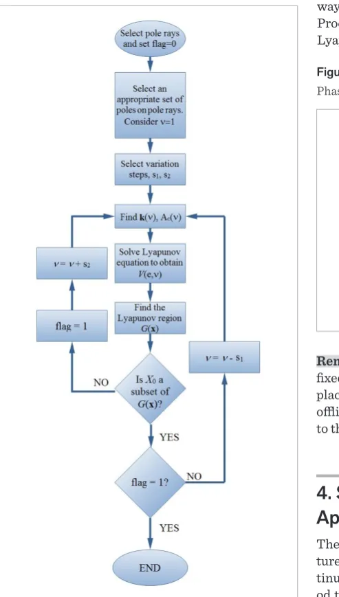
The flowchart of Procedure 1 is depicted in Figure 2.
Remark 1: Procedure 1 determines the smallest 𝑣𝑣𝑣𝑣
that yields a Lyapunov region that contains 𝑋𝑋𝑋𝑋0. The algorithm is initialized with a 𝑣𝑣𝑣𝑣 value that corresponds to a Lyapunov region that does not contain 𝑋𝑋𝑋𝑋0. It then progressively adds the variation
step, 𝑠𝑠𝑠𝑠2, and checks 𝑋𝑋𝑋𝑋0⊂ 𝐺𝐺𝐺𝐺 until it reaches an
optimum 𝑣𝑣𝑣𝑣 value. The flag prameter is defined to make the initialized value of 𝑣𝑣𝑣𝑣 small enough for
𝑋𝑋𝑋𝑋0⊄ 𝐺𝐺𝐺𝐺.
Remark 2:If the feasible initial condition set 𝑋𝑋𝑋𝑋0is a
subset of G, then this state feedback control vector will satisfy the input constraint. Since G is an invariant set and 𝑋𝑋𝑋𝑋0⊂G, the state trajectory cannot
leave the Lyapunov region of Step 4 and the input signal always satisfies (2). Figure 3, illustrates this situation. Procedure 1 tries to find the smallest νthat leads to a Lyapunov region G, where 𝑋𝑋𝑋𝑋0⊂G.
Figure 2
Flowchart of Procedure 1
(5)
then the control vector k(v) will be evaluated as fol-lows:
The following procedure determines the optimum feedback gain that provides a fixed structure, fast and stable control, and satisfies the input signal constraint (2).
Procedure 1: Initialize with a flag value flag=0.
Step 1: Select an appropriate pole ray considering the
desired or allowed overshoot as depicted in Figure 1.
Step 2: Select a suitable set of poles on the pole paths and
consider 𝑣𝑣𝑣𝑣= 1 for this set.
Step 3: Select suitable positive variation steps, 𝑠𝑠𝑠𝑠1 and
𝑠𝑠𝑠𝑠2with 𝑠𝑠𝑠𝑠2≪ 𝑠𝑠𝑠𝑠1< 1. For example, 𝑠𝑠𝑠𝑠1= 0.2 and 𝑠𝑠𝑠𝑠2= 0.02 would be appropriate.
Step 4: Find the feedback gain 𝐤𝐤𝐤𝐤𝑇𝑇𝑇𝑇(𝑣𝑣𝑣𝑣) that leads to a
closed loop system with the selected poles. If the state equation of the desired closed loop system is
𝐱𝐱𝐱𝐱̇=�𝐴𝐴𝐴𝐴 − 𝐛𝐛𝐛𝐛𝐤𝐤𝐤𝐤𝑇𝑇𝑇𝑇(𝑣𝑣𝑣𝑣)�𝐱𝐱𝐱𝐱=𝐴𝐴𝐴𝐴
𝑐𝑐𝑐𝑐(𝑣𝑣𝑣𝑣)𝐱𝐱𝐱𝐱, (5) then the control vector 𝐤𝐤𝐤𝐤(𝑣𝑣𝑣𝑣) will be evaluated as follows:
𝐤𝐤𝐤𝐤(𝑣𝑣𝑣𝑣) =�
𝑎𝑎𝑎𝑎�0𝜐𝜐𝜐𝜐−𝑛𝑛𝑛𝑛− 𝑎𝑎𝑎𝑎0 𝑎𝑎𝑎𝑎�1𝜐𝜐𝜐𝜐−(𝑛𝑛𝑛𝑛−1)− 𝑎𝑎𝑎𝑎1
⋮ 𝑎𝑎𝑎𝑎�𝑛𝑛𝑛𝑛−1𝜐𝜐𝜐𝜐−1− 𝑎𝑎𝑎𝑎𝑛𝑛𝑛𝑛−1
� , (6)
where 𝑎𝑎𝑎𝑎�𝑗𝑗𝑗𝑗, 𝑗𝑗𝑗𝑗= 0,1, … ,𝑛𝑛𝑛𝑛 −1, are the coefficients of the characteristic polynomial of 𝐴𝐴𝐴𝐴𝑐𝑐𝑐𝑐(𝑣𝑣𝑣𝑣= 1).
Step 5: Solve the Lyapunov equation (4) of the closed
loop system for the positive definite matrix, 𝑃𝑃𝑃𝑃, to obtain the Lyapunov function 𝑉𝑉𝑉𝑉(𝐱𝐱𝐱𝐱) =𝐱𝐱𝐱𝐱𝑇𝑇𝑇𝑇𝑃𝑃𝑃𝑃𝐱𝐱𝐱𝐱.
Step 6: Using the Lyapunov function, find a Lyapunov
region 𝐺𝐺𝐺𝐺= {𝐱𝐱𝐱𝐱|𝑉𝑉𝑉𝑉(𝐱𝐱𝐱𝐱) <𝑐𝑐𝑐𝑐} in which the input constraint is satisfied. To fully exploit the control signal, the hyperplanes ±𝐤𝐤𝐤𝐤𝑇𝑇𝑇𝑇𝐱𝐱𝐱𝐱=𝑢𝑢𝑢𝑢
0must be tangent to the Lyapunov region. To determine an appropriate 𝑐𝑐𝑐𝑐 value in the Lyapunov region formula, solve the optimization problem
max𝐱𝐱𝐱𝐱𝑇𝑇𝑇𝑇𝑃𝑃𝑃𝑃𝐱𝐱𝐱𝐱 𝐬𝐬𝐬𝐬.𝐭𝐭𝐭𝐭. |𝐤𝐤𝐤𝐤𝑇𝑇𝑇𝑇𝐱𝐱𝐱𝐱| <𝑢𝑢𝑢𝑢
0. (7) The solution of (7) is 𝑐𝑐𝑐𝑐=𝑢𝑢𝑢𝑢02/𝐤𝐤𝐤𝐤𝑇𝑇𝑇𝑇𝑃𝑃𝑃𝑃−1𝐤𝐤𝐤𝐤.
Step 7: If 𝑋𝑋𝑋𝑋0⊄ 𝐺𝐺𝐺𝐺, change 𝜐𝜐𝜐𝜐 to 𝜐𝜐𝜐𝜐=𝜐𝜐𝜐𝜐+𝑠𝑠𝑠𝑠2, set flag = 1, and go to Step 4.
Step 8: If 𝑋𝑋𝑋𝑋0⊂ 𝐺𝐺𝐺𝐺 and flag = 0, change the parameter 𝜐𝜐𝜐𝜐
to 𝜐𝜐𝜐𝜐=𝜐𝜐𝜐𝜐 − 𝑠𝑠𝑠𝑠1 and go to Step 4. If 𝑋𝑋𝑋𝑋0⊂ 𝐺𝐺𝐺𝐺 and flag = 1, stop.
The flowchart of Procedure 1 is depicted in Figure 2.
Remark 1: Procedure 1 determines the smallest 𝑣𝑣𝑣𝑣
that yields a Lyapunov region that contains 𝑋𝑋𝑋𝑋0. The algorithm is initialized with a 𝑣𝑣𝑣𝑣 value that corresponds to a Lyapunov region that does not contain 𝑋𝑋𝑋𝑋0. It then progressively adds the variation step, 𝑠𝑠𝑠𝑠2, and checks 𝑋𝑋𝑋𝑋0⊂ 𝐺𝐺𝐺𝐺 until it reaches an optimum 𝑣𝑣𝑣𝑣 value. The flag prameter is defined to make the initialized value of 𝑣𝑣𝑣𝑣 small enough for 𝑋𝑋𝑋𝑋0⊄ 𝐺𝐺𝐺𝐺.
Remark 2: If the feasible initial condition set 𝑋𝑋𝑋𝑋0 is a
subset of G, then this state feedback control vector will satisfy the input constraint. Since G is an invariant set and 𝑋𝑋𝑋𝑋0⊂G, the state trajectory cannot leave the Lyapunov region of Step 4 and the input signal always satisfies (2). Figure 3, illustrates this situation. Procedure 1 tries to find the smallest ν that leads to a Lyapunov region G, where 𝑋𝑋𝑋𝑋0⊂G.
Figure 2
Flowchart of Procedure 1
(6)
where a^j, j = 0,1, ..., n – 1, are the coefficients of the char-acteristic polynomial of Ac(v = 1).
Step 5: Solve the Lyapunov equation (4) of the closed loop system for the positive definite matrix, P, to ob-tain the Lyapunov function V(x) = xTPx.
Step 6: Using the Lyapunov function, find a Lyapunov region G = {x|V(x) < c} in which the input constraint is satisfied. To fully exploit the control signal, the hy-perplanes ±kTx = u
0 must be tangent to the Lyapunov region. To determine an appropriate c value in the Lyapunov region formula, solve the optimization problem
The following procedure determines the optimum feedback gain that provides a fixed structure, fast and stable control, and satisfies the input signal constraint (2).
Procedure 1: Initialize with a flag value flag=0.
Step 1: Select an appropriate pole ray considering the desired or allowed overshoot as depicted in Figure 1.
Step 2: Select a suitable set of poles on the pole paths and consider 𝑣𝑣 𝑣 𝑣 for this set.
Step 3: Select suitable positive variation steps, 𝑠𝑠� and 𝑠𝑠�with 𝑠𝑠�≪ 𝑠𝑠�< 𝑣. For example, 𝑠𝑠�𝑣 0.2 and
𝑠𝑠�𝑣 0.02 would be appropriate.
Step 4: Find the feedback gain 𝐤𝐤�(𝑣𝑣) that leads to a closed loop system with the selected poles. If the
state equation of the desired closed loop system is
𝐱𝐱� 𝑣 �𝐴𝐴 − �𝐤𝐤�(𝑣𝑣)�𝐱𝐱 𝑣 𝐴𝐴
�(𝑣𝑣)𝐱𝐱 , (5)
then the control vector 𝐤𝐤(𝑣𝑣) will be evaluated as follows:
𝐤𝐤(𝑣𝑣) 𝑣 �
𝑎𝑎��𝜐𝜐��− 𝑎𝑎�
𝑎𝑎��𝜐𝜐�(���)− 𝑎𝑎�
⋮
𝑎𝑎����𝜐𝜐��− 𝑎𝑎���
� , (6)
where 𝑎𝑎��, 𝑗𝑗 𝑣 0𝑗𝑣𝑗 𝑗 𝑗 𝑗𝑗 − 𝑣, are the coefficients of the characteristic polynomial of 𝐴𝐴�(𝑣𝑣 𝑣 𝑣).
Step 5: Solve the Lyapunov equation (4) of the closed loop system for the positive definite matrix, 𝑃𝑃, to
obtain the Lyapunov function 𝑉𝑉(𝐱𝐱) 𝑣 𝐱𝐱�𝑃𝑃𝐱𝐱.
Step 6: Using the Lyapunov function, find a Lyapunov region 𝐺𝐺 𝑣 �𝐱𝐱𝐱𝑉𝑉(𝐱𝐱) < 𝑐𝑐� in which the input
constraint is satisfied. To fully exploit the control signal, the hyperplanes ±𝐤𝐤�𝐱𝐱 𝑣 𝐱𝐱
�must be tangent to
the Lyapunov region. To determine an appropriate 𝑐𝑐 value in the Lyapunov region formula, solve the
optimization problem
max 𝐱𝐱�𝑃𝑃𝐱𝐱𝑃𝑃𝑃𝑃𝑃𝑃𝑃𝑃𝑃. 𝑃𝑃. 𝐱𝐤𝐤�𝐱𝐱𝐱 < 𝐱𝐱
�. (7)
The solution of (7) is 𝑐𝑐 𝑣 𝐱𝐱��/𝐤𝐤�𝑃𝑃��𝐤𝐤.
Step 7: If 𝑋𝑋�⊄ 𝐺𝐺, change 𝜐𝜐 to 𝜐𝜐 𝑣 𝜐𝜐 𝜐 𝑠𝑠�, set flag = 1, and go to Step 4.
Step 8: If 𝑋𝑋�⊂ 𝐺𝐺 and flag = 0, change the parameter 𝜐𝜐 to 𝜐𝜐 𝑣 𝜐𝜐 − 𝑠𝑠� and go to Step 4. If 𝑋𝑋�⊂ 𝐺𝐺 and flag
= 1, stop.
The flowchart of Procedure 1 is depicted in Figure 2.
Remark 1: Procedure 1 determines the smallest 𝑣𝑣 that yields a Lyapunov region that contains 𝑋𝑋�. The
algorithm is initialized with a 𝑣𝑣 value that corresponds to a Lyapunov region that does not contain 𝑋𝑋�. It
then progressively adds the variation step, 𝑠𝑠�, and checks 𝑋𝑋�⊂ 𝐺𝐺 until it reaches an optimum 𝑣𝑣 value. The
Information Technology and Control 2018/3/47 450
The following procedure determines the optimum feedback gain that provides a fixed structure, fast and stable control, and satisfies the input signal constraint (2).
Procedure 1: Initialize with a flag value flag=0.
Step 1: Select an appropriate pole ray considering the
desired or allowed overshoot as depicted in Figure 1.
Step 2: Select a suitable set of poles on the pole paths and
consider 𝑣𝑣𝑣𝑣= 1 for this set.
Step 3: Select suitable positive variation steps, 𝑠𝑠𝑠𝑠1 and
𝑠𝑠𝑠𝑠2with 𝑠𝑠𝑠𝑠2≪ 𝑠𝑠𝑠𝑠1< 1. For example, 𝑠𝑠𝑠𝑠1= 0.2 and 𝑠𝑠𝑠𝑠2=
0.02 would be appropriate.
Step 4: Find the feedback gain 𝐤𝐤𝐤𝐤𝑇𝑇𝑇𝑇(𝑣𝑣𝑣𝑣) that leads to a
closed loop system with the selected poles. If the state equation of the desired closed loop system is
𝐱𝐱𝐱𝐱̇=�𝐴𝐴𝐴𝐴 − 𝐛𝐛𝐛𝐛𝐤𝐤𝐤𝐤𝑇𝑇𝑇𝑇(𝑣𝑣𝑣𝑣)�𝐱𝐱𝐱𝐱=𝐴𝐴𝐴𝐴
𝑐𝑐𝑐𝑐(𝑣𝑣𝑣𝑣)𝐱𝐱𝐱𝐱, (5)
then the control vector 𝐤𝐤𝐤𝐤(𝑣𝑣𝑣𝑣) will be evaluated as follows:
𝐤𝐤𝐤𝐤(𝑣𝑣𝑣𝑣) =�
𝑎𝑎𝑎𝑎�0𝜐𝜐𝜐𝜐−𝑛𝑛𝑛𝑛− 𝑎𝑎𝑎𝑎0
𝑎𝑎𝑎𝑎�1𝜐𝜐𝜐𝜐−(𝑛𝑛𝑛𝑛−1)− 𝑎𝑎𝑎𝑎1
⋮ 𝑎𝑎𝑎𝑎�𝑛𝑛𝑛𝑛−1𝜐𝜐𝜐𝜐−1− 𝑎𝑎𝑎𝑎𝑛𝑛𝑛𝑛−1
� , (6)
where 𝑎𝑎𝑎𝑎�𝑗𝑗𝑗𝑗, 𝑗𝑗𝑗𝑗= 0,1, … ,𝑛𝑛𝑛𝑛 −1, are the coefficients of the
characteristic polynomial of 𝐴𝐴𝐴𝐴𝑐𝑐𝑐𝑐(𝑣𝑣𝑣𝑣= 1).
Step 5: Solve the Lyapunov equation (4) of the closed
loop system for the positive definite matrix, 𝑃𝑃𝑃𝑃, to obtain the Lyapunov function 𝑉𝑉𝑉𝑉(𝐱𝐱𝐱𝐱) =𝐱𝐱𝐱𝐱𝑇𝑇𝑇𝑇𝑃𝑃𝑃𝑃𝐱𝐱𝐱𝐱.
Step 6: Using the Lyapunov function, find a Lyapunov
region 𝐺𝐺𝐺𝐺= {𝐱𝐱𝐱𝐱|𝑉𝑉𝑉𝑉(𝐱𝐱𝐱𝐱) <𝑐𝑐𝑐𝑐} in which the input constraint is satisfied. To fully exploit the control signal, the hyperplanes ±𝐤𝐤𝐤𝐤𝑇𝑇𝑇𝑇𝐱𝐱𝐱𝐱=𝑢𝑢𝑢𝑢
0must be tangent to the Lyapunov
region. To determine an appropriate 𝑐𝑐𝑐𝑐 value in the Lyapunov region formula, solve the optimization problem
max𝐱𝐱𝐱𝐱𝑇𝑇𝑇𝑇𝑃𝑃𝑃𝑃𝐱𝐱𝐱𝐱 𝐬𝐬𝐬𝐬.𝐭𝐭𝐭𝐭.
|𝐤𝐤𝐤𝐤𝑇𝑇𝑇𝑇𝐱𝐱𝐱𝐱| <𝑢𝑢𝑢𝑢
0. (7)
The solution of (7) is 𝑐𝑐𝑐𝑐=𝑢𝑢𝑢𝑢02/𝐤𝐤𝐤𝐤𝑇𝑇𝑇𝑇𝑃𝑃𝑃𝑃−1𝐤𝐤𝐤𝐤.
Step 7: If 𝑋𝑋𝑋𝑋0⊄ 𝐺𝐺𝐺𝐺, change 𝜐𝜐𝜐𝜐 to 𝜐𝜐𝜐𝜐=𝜐𝜐𝜐𝜐+𝑠𝑠𝑠𝑠2, set flag = 1,
and go to Step 4.
Step 8: If 𝑋𝑋𝑋𝑋0⊂ 𝐺𝐺𝐺𝐺 and flag = 0, change the parameter 𝜐𝜐𝜐𝜐
to 𝜐𝜐𝜐𝜐=𝜐𝜐𝜐𝜐 − 𝑠𝑠𝑠𝑠1 and go to Step 4. If 𝑋𝑋𝑋𝑋0⊂ 𝐺𝐺𝐺𝐺 and flag
= 1, stop.
The flowchart of Procedure 1 is depicted in Figure 2.
Remark 1: Procedure 1 determines the smallest 𝑣𝑣𝑣𝑣
that yields a Lyapunov region that contains 𝑋𝑋𝑋𝑋0. The
algorithm is initialized with a 𝑣𝑣𝑣𝑣 value that corresponds to a Lyapunov region that does not contain 𝑋𝑋𝑋𝑋0. It then progressively adds the variation
step, 𝑠𝑠𝑠𝑠2, and checks 𝑋𝑋𝑋𝑋0⊂ 𝐺𝐺𝐺𝐺 until it reaches an
optimum 𝑣𝑣𝑣𝑣 value. The flag prameter is defined to make the initialized value of 𝑣𝑣𝑣𝑣 small enough for 𝑋𝑋𝑋𝑋0⊄ 𝐺𝐺𝐺𝐺.
Remark 2: If the feasible initial condition set 𝑋𝑋𝑋𝑋0 is a
subset of G, then this state feedback control vector will satisfy the input constraint. Since G is an invariant set and 𝑋𝑋𝑋𝑋0⊂G, the state trajectory cannot leave the Lyapunov region of Step 4 and the input signal always satisfies (2). Figure 3, illustrates this situation. Procedure 1 tries to find the smallest ν that leads to a Lyapunov region G, where 𝑋𝑋𝑋𝑋0⊂G.
Figure 2
Flowchart of Procedure 1
(7)
The solution of (7) is c = u2 0 /kTP–1k.
Step 7: If X0⊄G, change v to v = v + s2, set flag = 1, and go to Step 4.
Step 8:If X0⊂G and flag = 0, change the parameter v
to v = v – s1 and go to Step 4. If X0⊂G and flag = 1, stop.
The flowchart of Procedure 1 is depicted in Figure 2.Remark 2:satisfy the input constraint. Since If the feasible initial condition set 𝑋𝑋G is an invariant set and � is a subset of G, then this state feedback control vector will 𝑋𝑋�⊂ G, the state trajectory cannot leave the
Lyapunov region of Step 4 and the input signal always satisfies (2). Figure 3, illustrates this situation. Procedure 1 tries to find the smallest ν that leads to a Lyapunov region G, where 𝑋𝑋�⊂ G.
Figure 2
Flowchart of Procedure 1
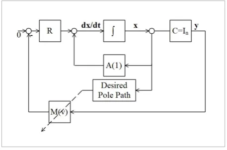
Remark 3: The method discussed in this section is a fixed structure control approach. Once the best pole placement, which satisfies the constraints, is found offline, the fixed respective control law will be applied to the plant.
Figure 3
Phase plane diagram of a second order system when 𝑋𝑋�⊂ 𝐺𝐺
Figure 2
Flowchart of Procedure 1
Remark 1:Procedure 1 determines the smallest v that yields a Lyapunov region that contains X0. The algo-rithm is initialized with a v value that corresponds to a Lyapunov region that does not contain X0. It then progressively adds the variation step, s2, and checks X0⊂G until it reaches an optimum v value. The flag prameter is defined to make the initialized value of v small enough for X0⊄G.
Remark 2: If the feasible initial condition set X0 is a subset of G, then this state feedback control vector will satisfy the input constraint. Since G is an invari-ant set and X0⊂ G, the state trajectory cannot leave the Lyapunov region of Step 4 and the input signal al-ways satisfies (2). Figure 3, illustrates this situation. Procedure 1 tries to find the smallest v that leads to a Lyapunov region G, where X0⊂G.
Figure 3
Phase plane diagram of a second order system when X0⊂G
Remark 3: The method discussed in this section is a fixed structure control approach. Once the best pole placement, which satisfies the constraints, is found offline, the fixed respective control law will be applied to the plant.