Image Classification Based on Effective Probabilistic Latent Semantic Analysis Model

(1)

Image Classification Based on Effective Probabilistic

Latent Semantic Analysis Model

D. Antony Pandiarajan

Assistant Professor,

Fatima Michael College of Engineering and Technology, Madurai Email:[email protected]

S. N. Nisharani

Assistant Professor,

Fatima Michael College of Engineering and Technology, Madurai

Abstract - This article proposes a new method for

classification of rock images using Tamura features and an effective topic generation model called probabilistic latent semantic analysis (PLSA). The rock textures can be very well represented by the six Tamura features known as coarseness, contrast, directionality, line likeness, regularity and roughness. A topic model is generated by applying Tamura features to PLSA. The Sum of Square Difference (SSD) classifier is employed for the classification process. The SSD classifier is applied over the topic model to classify the rock texture. This classification is compared with GLCM, color co occurrence and Tamura features methods. This method gives the accuracy of 74.33%.

Keywords – Rock Images, PLSA, Tamura Features, GLCM, Color Co Occurrence (CCM), SSD Classifier, Topic Model

I. I

NTRODUCTION

The texture of rock is stochastic in nature like most other natural textures. In addition to the stochastic nature of the rock textures, a more significant characteristic of the rock texture is non-homogeneity. Texture properties are significant in rock image analysis. Based on texture, it is possible to estimate several types of rock properties. For example, the visual properties of rock plates manufactured in the building industry are dependent on the texture of the rock surface. Texture directionality and granularity are very important texture properties in rock texture analysis. This is because several types of rock textures have strong directionality and granular size of the rock texture also often varies. Texture directionality and granularity are important factors in terms of human texture perception and therefore have a significant effect on the visual properties of a surface constructed of rock. In bedrock investigation directionality and granularity play a major role in the recognition of different rock types.

The rocks are mainly classified into three types. They are igneous, metamorphic and sedimentary. They are further classified into number of subclasses. Andesite, basalt, gabbro, granite and etc… are belonging to the type of igneous. Amphibolite, gneiss, marble, and etc… are belonging to the type of metamorphic. And breccia, chert, coal, siltstone and etc… are belonging to the type of sedimentary. The automated classification of rock images is an important task in rock industries and bedrock investigations. Compared to manual inspection and classification, the use of automated classification gives several benefits. Manual inspection carried out by the people might be affected by the factors such as personal preferences, fatigue, and the concentration level of the

individual doing the task. By contrast automatic classification is more dependable and consistent method.

In previous works the classification has been done based on spectral and textural features of the rocks [8].The spectral features are considered as some color parameters whereas the textural features are calculated from the co-occurrence matrix. Leena Lepisto et al. [7], applied Gaussian band pass filtering to extract the color features of the images in RGB and HSI color spaces. In [6], texture features are extracted by Haralick features [17] from co occurrence matrix of the image and the color features are extracted by mean, variance, skewness. Laercio B. Goncalves and Fabiana R. Leta [5], did the image classification for macroscopic rocks based on texture descriptors, such as spatial variation coefficient, Hurst co efficient, entropy, and co occurrence matrix.

In nature some features of some rocks from different classes might be same. In all those methods the features of the rock textures are extracted and they are directly applied to the classifier. Due to this, the classification of few rock textures may give false result. Since the accuracy of classification is very less. This can be overcome by Probabilistic Latent Semantic Analysis (PLSA) [19].

PLSA is a novel statistical technique for the analysis of two mode and co-occurrence data, which has applications in information retrieval and filtering, natural language processing, machine learning from text, and in related areas. This PLSA method is based on a mixture decomposition derived from a latent class model. This results in a more principled approach which has a solid foundation in statistics. In order to avoid over fitting, a widely applicable generalization of maximum likelihood model fitting by EM is proposed.

(2)

image annotation is done based on the latent space. Peng Y.X. et al. [14] constructed an audio vocabulary and proposed an audio PLSA model for semantic concept annotation.

II. P

ROPOSED

M

ETHOD

In this section, the proposed methodology for the classification of rock textures has been discussed. This classification method takes the advantage of probabilistic latent semantic analysis (PLSA).

A. Classification method

Figure.1 depicts the proposed classification methodology. In the first step certain features of the texture called Tamura features are calculated for the query image.

Fig.1. Flowchart of rock image classification Similarly Tamura features are calculated for the rock images of three types known as igneous, metamorphic, and sedimentary.

These three set of features are used as training sequences. Then Bag of Words (or word image matrix) is formed using these three set of features and features of the query image. This word image matrix is applied for the generation of topic model using the popular probabilistic latent semantic analysis (PLSA) method. The final step is classification process using sum of square difference classifier by applying the topic model, which is generated from PLSA.

B. Features extraction

In the feature extraction process Tamura features are calculated for the query image. The Tamura features are a) Coarseness

b) Contrast c) Directionality d) Line likeness

e) Regularity f) Roughness

Coarseness:

Coarseness is the most fundamental feature in texture analysis; it refers to texture granularity, that is, the size and number of texture primitives. A coarse texture contains a small number of large primitives, whereas a fine texture contains a large number of small primitives. Coarseness (fcrs) can be computed as follows.



 n

i n

j k

crs p i j

n

f 2 (, )

2 … (1)

Where n x n denotes the image size, the sum is carried out for every pixel p (i, j) and k is obtained as the value which maximizes the differences of the moving averages taken over an 2k2k neighborhood, along the horizontal and vertical directions. In this study, k = 1, 2, 3, 4, and 5.

Contrast:

Contrast stands for image quality in the narrow sense; it refers the difference in intensity among neighboring pixels. A texture on high contrast has large difference in intensity among neighboring pixels, whereas a texture on low contrast has small difference. Contrast (fcon) can be computed as follows.

4 / 1

4 4_

     

   con

f ... (2)

Where σ is the image standard deviation and



₄ is fourth moment of the image.

Directionality:

Directionality is a global property over a specific region; it refers the shape of texture primitives and their placement rule. A directional texture has one or more recognizable orientation of primitives, whereas an isotropic texture has no recognizable orientation of primitives. Directionality (fdir) can be computed as follows.

dir

f

=

 



  p

n

p w_p

D p

p H

n r



) . ( )

( . .

1 2 … (3)

where H_D is the local direction histogram, n_p is the number of peaks of H_D,



_p is the p th peak position of

D

H , w_p is the range of p th peak between valleys, r is a normalizing factor, and



is the quantized direction code. In this study, the number of bins for H_D is 16, the quantized direction code



= 0, 1, 2. . . . 15, and the normalizing factor r =0.025.

Line-likeness:

Line-likeness refers only the shape of texture primitives. A line-like texture has straight or wave-like primitives whose orientation may not be fixed. Often the line-like texture is simultaneously directional. Line-likeness (flin) can be computed as follows.

 



 _n

i n

j Dd n

i n

j Dd lin

j i p

n j i j i p

f

) , (

] 2 ) cos[( ) ,

( 

(3)

co-occurrence matrix of points at a distance d.

Regularity:

Regularity refers to variations of the texture-primitive placement. A regular texture is composed of identical or similar primitives, which are regularly or almost regularly arranged. An irregular texture is composed of various primitives, which are irregularly or randomly arranged (Haralick, 1982). Regularity (freg) can be computed as follows.

)

(

1

_crs _con _dir _lin

reg

r

f



















… (5)

Where r is a normalizing factor and



_xxx means the standard deviation of

f

_xxx. In this study, the normalizing factor r = 0.25.

Roughness:

Roughness refers tactile variations of physical surface. A rough texture contains angular primitives, whereas a smooth texture contains rounded blurred primitives. Roughness (frgh) can be computed as follows.

con crs

rgh

f





… (6)

C. Training set generation

In The training sequence generation process the same Tamura features are calculated for the three types of rock images i.e. igneous, metamorphic and sedimentary. These three set of features are used as training sequences.

Mostly the texture of metamorphic rocks is fine texture. Igneous rocks have coarse texture. Since the maximum value of coarseness, sedimentary rock textures are very coarse textures. Similarly the contrast of sedimentary rocks is less than that of others and the igneous is a more contrast texture. Metamorphic rocks are medium line like texture, igneous rocks are line like and sedimentary rocks are very line like textures. Mostly the metamorphic rocks are smooth textures, igneous rocks are medium rough and sedimentary rocks are very rough textures. Metamorphic rocks are more directional and sedimentary rocks are less directional compared to igneous rock texture. There is less regularity in igneous rocks. Metamorphic textures are medium regular and sedimentary rocks are most regular textures. These different properties of the training rock textures help in classification.

D. Topic model generation using PLSA

The PLSA model was originally developed for topic discovery in a text corpus, where each document is represented by its word frequency. The core of PLSA model is to map high dimensional word distribution vector of a document to a lower dimensional topic vector. Therefore, PLSA introduces a latent topic variable between the document d_i{d₁....d_n}and the word

} ....

{ ₁ _m

j w w

w  . Then the PLSA model is given by the following generative scheme

1. Select a document d_iwith probability p(d_i) 2. Pick a latent topic z_kwith probability p(z_k/d_i) 3. Generate a word w with probabilityj p(wj/zk). The model is graphically shown in the fig.2

Fig.2. PLSA model

Here the three types of rock are considered as documents. The latent topic is the sub classes of rocks such as andesite, basalt, gabbro, coal, granite, amphibolites, and gneiss. The set of Tamura features calculated for the query image and the training rock images are considered as words. This is depicted as follows.

Document  class of rock image Latent topic  subclass of rock image Word  feature of rock image.

As a result one obtain an observation pair (d_i,w ) while_j the latent topic variable is discarded. This generative model can be expressed by the following probabilistic model ) / ( ) ( ) ,

(w_j d_i p d_i p w_j d_i

p  … (7)

Where p(w_j/d_i)





 K k 1

) / (w_j z_k

p p(z_k/d_i) … (8)

The unobservable probability distribution p(z_k/d_i)and )

/ (wj zk

p are learnt from the complete dataset using expectation maximization (EM) algorithm [19]. The log likelihood of the complete dataset is



 n(d_i,w_j)logp(d_i,w_j)

L … (9)





   N i M j K k i k k j j

i w p w z p z d d

n

1 1 1

) / ( ) / ( log ) ,

( … (10)

Where n(d_i,w_j)is value of the visual word occurred in the word image matrix ‘n’. Each row in the matrix represents an image. The first row corresponds to the features of the query image and remaining rows are corresponds to the reference images i.e. training sequences.

The E- step is given by



  _K l i l l j i k k j j i k d z p z w p d z p z w p w d z p 1 ) / ( ) / ( ) / ( ) / ( ) , /

( … (11)

and M- step is given by





    N i M j j i k j i j i k N i j i k j w d z p w d n w d z p w d n z w p 1 1 1 ) , / ( ) , ( ) , / ( ) , ( ) /

( … (12)



   _M j j i M j j i k j i i k w d n w d z p w d n d z p 1 1 ) , ( ) , / ( ) , ( ) /

(4)

By randomly choosing initial values for p(w_j/z_k) and )

/ (z_k d_i

p iteratively perform E-step and M-step until the probability values are stable or up to 150 iterations. Then final values of p(z_k/d_i) and p(w_j/z_k) are applied to equation ofp(wj/di). Finally the topic model is generated using obtained values of p(w_j/d_i).

E. Classification

The first column in the generated topic model corresponds to the query image. The second, third and fourth columns of the topic model are correspond to the reference images igneous, metamorphic and sedimentary respectively. The classifier used in this classification process is Sum of Square Difference (SSD). In SSD classifier the corresponding difference between the first column of the topic model matrix i.e. topic model of the query image and each other columns is obtained. Then finally three SSD values will be obtained for query image with corresponds to training images of igneous, metamorphic and sedimentary rock types. The particular SSD value of topic model of the query image with that of the reference image will have least value when compare to other SSD values since the topic models of the same class of rock images would have similar values. Then the class of rock image will be declared as class of the training image with least SSD value of topic model.

III. E

XPERIMENTS AND

D

ISCUSSION

To demonstrate the significance of the proposed approach, a set of rock image classification experiments have been conducted. In which the query image of particular rock to be classified is retrieved from database. The six Tamura features are calculated for the query image. Then the rock images of andesite, amphibolite, and breccia from igneous, metamorphic, and sedimentary types respectively are considered as training or reference images. From which training samples are generated using the same Tamura method. Further the topic model is generated using PLSA method. The generated model is applied to SSD classifier. Finally a set three SSD value’s corresponds to igneous, metamorphic and sedimentary will be obtained. Among them one of three SSD value will be smaller. Then the class of the query rock image can be revealed as type of that minimum SSD value.

Fig.3. Various rock textures

Some of the rock images are shown in figure 3. The two set of training sequences i.e. features of the reference images are shown in table 1.1 and 1.2. From the table it can be inferred that mostly the textures of metamorphic rocks are fine textures, since it has less value of coarseness. Igneous rocks have coarse texture.

Table 1.1: Tamura Features of rock images. Classes of

Rocks

Igneous (Gabbro)

Metamor-Phic (Gneiss)

Sediment-ary (chert) Features of

rock images

Coarseness 0.5318 0.2873 0.9125

Contrast 0.0020 0.0018 8.0387e-005

Line likeness 0.5607 0.5208 0.9755

Roughness 0.5337 0.2890 0.9125

Directionality 1.0866 1.1260 1.0010

Regularity 0.4692 0.6932 0.9043

Table 1.2: Tamura Features of rock images. Classes of

Rocks

Igneous (Scoria)

Metamor-Phic (Muscovite

Schist)

Sediment-Ary (Shale) Features of

Rock Images

Coarsene-ss 0.5864 0.4390 0.9246

Contrast 0.0033 0.0020 9.1630e-005

Line likeness 0.7133 0.5076 0.9840

Roughness 0.5897 0.4410 0.9247

Directionality 1.1126 1.1313 1.0021

Regularity 0.3452 0.5258 0.8652

Since the maximum value of coarseness, sedimentary rock textures are very coarse textures. Similarly the contrast of sedimentary rocks is less than that of others and the igneous is a more contrast texture. Metamorphic rocks are medium line like texture, igneous rocks are line like and sedimentary rocks are very line like textures. Mostly the metamorphic rocks are smooth textures, igneous rocks are medium rough and sedimentary rocks are very rough textures. Metamorphic rocks are more directional and sedimentary rocks are less directional compared to igneous rock texture. There is less regularity in igneous rocks. Metamorphic textures are medium regular and sedimentary rocks are most regular textures. These differences in properties of the three types of rock textures are utilized in classification.

(5)

to the class of igneous. Similarly the experiment has been conducted for number of rock images. The calculated SSD values are shown in table.

The performance of the proposed approach is compared with other three methods. They are GLCM, color co occurrence and simple Tamura methods.

In GLCM method, the features of the rock images are extracted by 7 Haralick features, calculated from gray level co occurrence matrix. The Haralick features are angular second moment or energy, contrast, correlation, inverse difference moment, entropy, sum entropy, and sum average. Similarly the training sequences are generated for three reference images each from igneous, metamorphic and sedimentary. Finally in the classification process, three SSD values from features of the query image with training sequence are obtained. Remaining steps are same as that of PLSA method. Results are shown in table 3.

Color co occurrence method is similar to the GLCM method. Instead of calculating Haralick features from GLCM matrix, they are calculated from color co occurrence matrix. Color co occurrence matrix is generated by separating the given rock image into R, G, and B channels. Then 3 co occurrence matrices are obtained for the combinations of RG, GB, and BR. Corresponding three set of features are averaged. Finally we have a set of 7 Haralick features. Remaining steps are same as that of GLCM method. Results are shown in table 4.

Tamura features method is exactly same as the proposed approach. But instead of generating topic model in the PLSA process, the six Tamura features are directly applied to the classification process. Results are shown in table 5. Accuracy of these methods is calculated as follows. Classification Accuracy

=

Accuracies of those methods are compared using bar chart and also in line chart, which is shown in figure 3.

Table 2: Sum of Square Distance for various rock images using PLSA.

Reference Images

Igneous (andesite)

Metamor-phic

(Amphibol-ite)

Sedimentary (Breccia) Query

Images

Andesite 1.1661e-019 0.0012 9.5456e-005

Basalt 1.3053e-004 0.0020 1.3838e-004

Gabbro 2.5505e-004 3.3203e-004 3.7136e-004

Granite 2.5998e-004 3.6029e-004 2.9114e-004

Scoria 1.1701e-004 6.5165e-004 1.1781e-004

Peridotite 9.1263e-006 0.0010 6.3558e-005

Pumice 6.1860e-005 0.0012 6.1909e-006

Amphibol-ite

0.0012 1.7896e-018 0.0013

Gneiss 0.0017 1.2492e-004 0.0016

Marble 2.0498e-004 0.0022 1.5055e-004

Muscovite -schist

6.9861e-004 5.9748e-005 8.0689e-004

Chlorite-schist

1.5853e-004 7.9780e-004 4.3966e-004

Breccia 9.5455e-005 0.0013 1.2839e-014

Chert 3.1619e-004 0.0026 2.9632e-004

Phyllite 1.8274e-004 0.0022 1.6573e-004

Coal 1.3397e-004 0.0018 5.3444e-005

Shale 3.3660e-004 0.0027 3.1744e-004

Hematite 4.9359e-005 0.0016 6.2437e-005

Siltstone 2.7617e-004 0.0025 2.5783e-004 Bold values indicate the place where the minimum sum of square distance achieved.

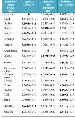
Table 3: Sum of square distance for various rock images using GLCM.

Reference images

Metamor-phic

(Amphibol-ite)

Sediment-ary (Breccia) Query

images

Andesite 0 5.5696e+019 1.7095e+019

Basalt 1.5428e+019 1.2975e+020 4.2738e+016

Gabbro 3.0965e+018 3.2527e+019 3.4743e+019

Granite 2.1000e+019 8.2970e+018 7.5988e+019

Scoria 9.6426e+017 4.2003e+019 2.6179e+019

Peridotite 5.2353e+017 6.7019e+019 1.1635e+019

Pumice 8.1885e+017 7.0021e+019 1.0431e+019

Amphibolite 5.5696e+019 0 1.3450e+020

Gneiss 3.8546e+019 1.5735e+018 1.0698e+020

Marble 1.5101e+019 1.2880e+020 6.1818e+016

Muscovite-schist

5.5696e+019 1.3152e+010 1.3450e+020

Chlorite-schist

2.3722e+019 6.7205e+018 8.1093e+019

Breccia 1.7095e+019 1.3450e+020 0

Chert 2.5658e+019 1.5696e+020 8.6640e+017

Phyllite 8.9762e+018 1.0939e+020 1.2964e+018

Coal 2.3063e+019 1.5044e+020 4.4597e+017

Shale 2.4031e+019 1.5289e+020 5.8904e+017

Hematite 3.2242e+018 8.5721e+019 5.4710e+018

(6)

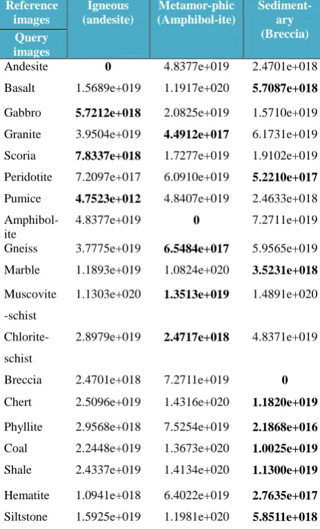
Table 4: Sum of square distance for various rock images using CCM.

Metamor-phic (Amphibol-ite)

Sediment-ary (Breccia) Query

images

Andesite 0 4.8377e+019 2.4701e+018

Basalt 1.5689e+019 1.1917e+020 5.7087e+018

Gabbro 5.7212e+018 2.0825e+019 1.5710e+019

Granite 3.9504e+019 4.4912e+017 6.1731e+019

Scoria 7.8337e+018 1.7277e+019 1.9102e+019

Peridotite 7.2097e+017 6.0910e+019 5.2210e+017

Pumice 4.7523e+012 4.8407e+019 2.4633e+018

Amphibol-ite

4.8377e+019 0 7.2711e+019

Gneiss 3.7775e+019 6.5484e+017 5.9565e+019

Marble 1.1893e+019 1.0824e+020 3.5231e+018

Muscovite

-schist

1.1303e+020 1.3513e+019 1.4891e+020

Chlorite-schist

2.8979e+019 2.4717e+018 4.8371e+019

Breccia 2.4701e+018 7.2711e+019 0

Chert 2.5096e+019 1.4316e+020 1.1820e+019

Phyllite 2.9568e+018 7.5254e+019 2.1868e+016

Coal 2.2448e+019 1.3673e+020 1.0025e+019

Shale 2.4337e+019 1.4134e+020 1.1300e+019

Hematite 1.0941e+018 6.4022e+019 2.7635e+017

Siltstone 1.5925e+019 1.1981e+020 5.8511e+018

Table 5: Sum of square distance for various rock images using Tamura features.

Metamor-phic (Amphibol-ite)

Sediment-ary (Breccia) Query

images

Andesite 0 0.2748 0.0262

Basalt 0.0691 0.6002 0.0706

Gabbro 0.0769 0.0616 0.1063

Granite 0.0808 0.0655 0.0892

Scoria 0.0309 0.1530 0.0314

Peridotite 0.0025 0.2448 0.0174

Pumice 0.0172 0.2620 0.0022

Amphibol-ite 0.2748 0 0.3033

Gneiss 0.3787 0.0219 0.3679

Marble 0.0939 0.6551 0.0764

Muscovite-schist 0.1797 0.0101 0.2061

Chlorite-schist 0.0558 0.1526 0.1267

Breccia 0.0262 0.3033 0

Chert 0.1695 0.8573 0.1616

Phyllite 0.0856 0.6469 0.0795

Coal 0.0665 0.5303 0.0416

Shale 0.1847 0.8919 0.1773

Hematite 0.0177 0.4117 0.0211

Siltstone 0.1447 0.7997 0.1378

0 10 20 30 40 50 60 70 80

Cl

as

si

fi

ca

ti

on

A

c

cu

ra

cy

PLSA GLCM CCM TAMURA

Fig.3.1. Accuracy comparison

40 45 50 55 60 65 70 75 80

Cl

as

si

fi

ca

ti

on

A

c

cu

ra

cy

PLSA GLCM CCM TAMURA

Fig.3.2. Accuracy comparison Table 6: Accuracy

Alg

o

rit

h

m

T

am

u

ra

GL

C

M

C

o

lo

r

co

o

cc

u

rr

en

ce

P

ro

p

o

se

d

alg

o

rith

m

Overall Accuracy (%)

61.667 65.667 72.00 74.333

(7)

IV. C

ONCLUSION

In this paper, a novel method for classification of rock images has been proposed. The features of the rock images are very well extracted by Tamura features. These features are applied to probabilistic latent semantic analysis to generate a topic model, the effective generative model. This is computationally effective and more efficient generative model. Then topic model is applied to the SSD classifier, which is a simple classifier. Experimental results show that the proposed algorithm achieves high classification accuracy for the rock images. Hence this method can be directly applied to the rock industries for the classification of rock images and in bedrock investigations. Further improvement could be on, finding and applying a better classifier.

A

CKNOWLEDGMENT

The authors are very much thankful to the reviewers for their valuable comments and also to the Management and Department of Electronics and Communication Engineering of Thiagarajar College of Engineering for their support and assistance to carry out this work.

R

EFERENCES

[1] Bosch, A., Zisserman, A., Munoz, X.: Scene classification via PLSA. In Proc. of the European Conference on Computer Vision. (2006).

[2] Heather Dunlop, Automatic Rock Detection and Classification in Natural Scenes. (2006)

[3] Jing Yi Tou, Yong Haur Tay, Phooi Yee Lau, Recent trends in texture classification.

[4] L. Lepisto, I. Kuntu, A, Visa, Rock image classification based on k- nearest neighbor voting. (2006)

[5] Laercio B. Goncalves, and Fabiana R. Leta, Macroscopic Rock Texture Image Classification Using a Hierarchical Neuro Fuzzy Class Method. (2010)

[6] Leena Lepisto, Colour and Texture Based Classification of Rock Images Using Classifier Combinations. (2006)

[7] Leena Lepisto, Iivari Kunttu, Ari Visa, Rock image classification using color features in Gabor space. (2005)

[8] Leena Lepisto, Iivari Kunttu, Jorma Autio, and Ari Visa, Rock Image Classification Using Non-Homogenous Textures and Spectral Imaging. (2003)

[9] Lu, Z.W., Peng, Y.X., Horace, H.S.Ip. Image categorization via robust pLSA. Pattern Recognition Letters 31(1), 36-43. (2010) [10] Mari Partio, Bogdan Cramariuc, Moncef Gabbouj, and Ari Visa,

Rock texture retrieval using gray level co-occurrence matrix,. [11] Mona Sharma, Markos Markou, Sameer Singh, Evaluation of

texture methods for image analysis.

[12] Monay, F., Gatica-Perez, D. PLSA-based image auto-annotation constraining the latent space. In Proceedings of ACM international conference on multimedia, pp. 348–351. (2004) [13] P.Paclik, S.Verzakov, R.P.W.Duin, Improving the

maximum-likelihood co-occurrence classifier, a study on classification of inhomogeneous rock images. (2006)

[14] Peng, Y.X., Lu, Z.W., Xiao, J.G. Semantic concept annotation based on audio PLSA model. In Proceedings of ACM International Conference on Multimedia, pp. 841-844. (2009) [15] R.F. Walker, P.T. Jackway, I.D. Longstaff, Recent development

in the use of co–occurrence matrix for texture recognition. (2000)

[16] Rainer, L., Stefan, R., Eva, H. Multilayer PLSA for multimodal image retrieval. In Proceedings of the ACM International Conference on Image and Video Retrieval. (2009)

[17] Robert M. Haralick, K. Shanmugam, and Its’hak Dinstein,

Texural features for image classification, IEEE Transaction on systems, man and cybernatics, pp. 610-621. (1973)

[18] Shah-hosseini, A., Knapp, G. Semantic image retrieval based on probabilistic latent semantic analysis. In: Proceedings of ACM International Conference on Multimedia, pp. 452-455. (2004) [19] Thomas Hofmann, Probabilistic Latent Semantic Analysis,

Uncertainty in Artificial Intelligence, UAI'99, Stockholm. [20] Zhang, R.F., Zhang, Z.F. Effect image retrieval based on hidden

concept discovery in image database. IEEE Transactions on Image Processing 16(2), 562-572. (2007)

A

UTHOR

’

S

P

ROFILE

Mr. D. Antony Pandiarajan

working as an Assistant Professor in Fatima Michael College of Engineering & Technology, Madurai. He received his M.E degree in Communication Systems in Thiagarajar College of Engineering, Tamilnadu, India. He received his B.E degree in Electronics and Communication Engg. at College of Engg, Guindy, Anna University, Chennai. His research interests include Image Processing, Wireless Network Security and MANET.

Image Classification Based on Effective Probabilistic Latent Semantic Analysis Model