A Study on Functional Fractional Integro-Differential Equations of
Hammerstein type
Leila Saeedi
Department of Mathematics, Shahed University, Tehran, Iran.
E-mail: [email protected], [email protected]
Abolfazl Tari∗
Department of Mathematics, Shahed University, Tehran, Iran.
E-mail: [email protected], [email protected]
Esmail Babolian
Department of Computer Science, Kharazmi University, Tehran, Iran. E-mail: [email protected]
Abstract In this paper, functional Hammerstein integro-differential equations of fractional order is studied. Here the existence and uniqueness of the solution is proved. A numerical method to approximate the solution of problem is also presented which is based on an improvement of the successive approximations method. Error estimation of the method is analyzed and error bound is obtained. The convergence and stability of the method are proved. At the end, application of the method is revealed by presenting some examples.
Keywords. Functional Hammerstein integrao-differential equations, Fractional order, Successive approx-imations, Spline interpolation, Trapezoidal quadrature rule.
2010 Mathematics Subject Classification. 65R20, 97N40. 1. Introduction
Fractional integro-differential equations arise in modeling many processes in ap-plied sciences such as physics, chemistry, economy, electromagnetic, biology, engi-neering. Mathematical formulas of many phenomena such as oscillation of earth-quake, fluid-dynamic traffic, statistical mechanics, astronomy, control theory and other areas of application contain integro-differential equations of fractional order [5,6,7, 8,15,16,19,31, 32].
On the other hand, solution of most of these equations can not be obtained ana-lytically, so approximate methods should be used to solve them. For this type of equations, various methods have been used. For example, the Adomian decomposi-tion method [14, 27, 28, 33], variational iteration method and homotopy perturba-tion method [2, 13, 23, 29, 37], Taylor expansion [17], wavelets [26, 34, 38, 39, 41],
Received: 9 October 2018 ; Accepted: 22 December 2018.
∗corresponding author.
operational Tau method [21, 40], fractional differential transform method [4, 30], sinc-collocation method [3,12], Laplace transform method [20,22] and least squares method [25]. But, numerical solution of functional fractional integro-differential equa-tions of Hammerstein type, have been studied in a few references.
In this paper, we consider functional fractional Hammerstein integro-differential equa-tions (FFHIDEs) as
Dαy(t)−
Z b
a
K(t, s)F(s, y(s), y(θ(s)))ds=g1(t), t∈[a, b] (1.1)
with initial condition
y(a) =y0, (1.2)
where Dα denotes the Caputo fractional operator of order α, 0< α < 1, a, b ∈R, a < b,θ: [a.b]→[a, b],∀t∈[a, b], θ,g1∈C1[a, b], andK∈C1([a, b]×[a, b]).
Here, we combine the successive approximations method with the trapezoidal quadra-ture and natural cubic spline interpolation to solve the mentioned equations. Proving the convergence and numerical stability of the method only requires the Lipschitz properties.
2. Preliminary Results
2.1. Preliminaries. Assuming thatF ∈C1([a, b]×
R×R),K∈C1([a, b]×[a, b]),θ
andg∈C1[a, b] andθ: [a, b]→[a, b]. Consider the following conditions:
(i) there exist λ, µ≥0 such that
|F(s, x1, z1)−F(s, x2, z2)| ≤λ|x1−x2|+µ|z1−z2|, (2.1)
for alls∈[a, b], (x1, z1),(x2, z2)∈R×R,
(ii)
2Q(b−a)q(λ+µ)<Γ(α+ 1) (2.2)
whereQ=max{|K(t, s)|,|∂K∂t(t,s)|: (t, s)∈[a, b]×[a, b]}and
(b−a)q =max{(b−a)α+1,(b−a)α+2}.
LetF0: [a, b]→R,F0(s) =F(s, g(s), g(θ(s))), thenF0 is continuous on the compact set [a, b] because F, g and θ are continuous and so there exists M ≥ 0, such that
|F0(s)|≤M for alls∈[a, b].
2.2. Basic definitions of fractional calculus. We recall the following definitions from [11]:
Definition 2.1. Letα∈R+. The operatorJ0α, defined on the space L1[a, b] by
Jaαf(t) := 1 Γ(α)
Z t
a
(t−x)α−1f(x)dx, Ja0f(t) =f(t). (2.3)
for a ≤ t ≤ b, is called the Riemann-Liouville fractional integral operator of order
Definition 2.2. The fractional derivative off in the Caputo sense is defined by
Dαaf(t) =J n−α
a D
n
f(t) = 1 Γ(n−α)
Z t
a
(t−x)n−α−1d
nf(x)
dxn dx, (2.4)
n−1< α≤n, n∈N, a≤t≤b, x >0.
3. Existence and uniqueness of the solution
In this section, the existence and uniqueness of the solution of problem (1.1)-(1.2) are investigated.
Lemma 3.1. Problem (1.1)-(1.2)is equivalent to the integral equation of the Ham-merstein type
y(t) =g(t) + Z t
a
H(t, s)F(s, y(s), y(θ(s)))ds (3.1)
where
g(t) =y(a) + 1 Γ(α)
Z t
a
(t−τ)α−1g1(τ)dτ,
H(t, s) = 1 Γ(α)
Z b
a
(t−τ)α−1K(τ, s)dτ.
In other words, every solution of the integral equation (3.1)is a solution of problem
(1.1)-(1.2), and vice versa.
Proof. Using the fractional integral operator on both sides of the equation (1.1) and by using of (1.2), we have
y(t) =y(a) + 1 Γ(α)
Z t
a
(t−τ)α−1g1(τ)dτ
+ 1
Γ(α) Z t
a
(t−τ)α−1 Z b
a
K(τ, s)F(s, y(s), y(θ(s)))dsdτ. (3.2)
By changing the order of integration in (3.2), equation (3.1) is obtained.
Remark 3.2. If the functionsg1 andKare continuous on their domains, thengand
H are also continuous.
Now we prove the existence and uniqueness of the solution by inspiration of [24].
Theorem 3.3. Ifg andH are continuous functions on[a, b]and[a, b]×[a, b] respec-tively, then the equation (3.1)has a unique continuous solution.
Proof. We define the sequence{yn(t)}∞
n=1 as follows:
yn(t) =g(t) +
Z t
a
H(t, s)F(s, yn−1(s), yn−1(θ(s)))ds, n= 1,2, ..., (3.3)
wherey0(t) =g(t). We introduce the sequenceψn(t) as follows:
whereψ0(t) =g(t) and so we have
yn(t) = n
X
i=0
ψi(t). (3.5)
By settingH1= max
t,s∈[a,b]|H(t, s)|and due to theθ: [a, b]→[a, b], we have
|ψn(t)|=|yn(t)−yn−1(t)|≤H1 Z t
a
λ|yn−1(s)−yn−2(s)|ds
+H1 Z t
a
µ|yn−1(θ(s))−yn−2(θ(s))|ds
≤H1(λ+µ) Z t
a max
s∈[a,b]|yn−1(s)−yn−2(s)|ds
=H1(λ+µ) Z t
a max s∈[a,b]
|ψn−1(s)|ds, n= 1,2, . . . .
Now, by using induction, we prove the following inequality:
|ψn(t)| ≤
G(H1(λ+µ)(t−a))n
n! , n= 0,1,2, ..., (3.6) whereG= maxt∈[a,b]|g(t)|.Obviously, the inequality holds forn= 0. Suppose that the inequality holds forn−1, we have:
|ψn(t)| ≤H1(λ+µ) Z t
a
|ψn−1(s)|ds
≤H1(λ+µ) Z t
a
G(H1(λ+µ)(s−a))n−1
(n−1)! ds
= G(H1(λ+µ))
n
(n−1)! Z t
a
(s−a)n−1ds
= G(H1(λ+µ)(t−a))
n
n! , n= 1,2, . . . .
Therefore, the sequenceyn(t) in (3.5) is uniformly convergent and can be written as:
y(t) = ∞ X
i=0
ψi(t). (3.7)
Now, we show that the continuous functiony(t) in (3.7) satisfies the equation (3.1). For this purpose, we put
y(t) =yn(t) + ∆n(t), (3.8)
by using (3.3), we have
y(t)−∆n(t) =g(t) +
Z t
a
H(t, s).F(s, y(s)−∆n−1(s), y(θ(s))
so that
y(t)−g(t)−
Z t
a
H(t, s).F(s, y(s), y(θ(s)))ds= ∆n(t) +
Z t
a
H(t, s)
.[F(s, y(s)−∆n−1(s), y(θ(s))−∆n−1(θ(s)))−F(s, y(s), y(θ(s)))]ds.
By applying (2.1), we have
|y(t)−g(t)−
Z t
a
H(t, s).F(s, y(s), y(θ(s)))ds|
≤|∆n(t)|+H1
λ
Z t
a
|∆n−1(s)|ds+µ
Z t
a
|∆n−1(θ(s))|
≤|∆n(t)|+H1(λ+µ)
Z t
a max
s∈[a,b]|∆n−1(s)|ds
≤|∆n(t)|+H1(t−a)(λ+µ)k∆n−1k,
wherek∆n−1k= max
a≤s≤b|∆n−1(s)|. On the other handnlim→∞|∆n−1|= 0, Therefore, for sufficiently large values ofn, the right-hand side of the inequality can be made as small as desired, and this concludes that the functiony(t) defined in the (3.7) satisfies the equation (3.1), and therefore is a solution of (3.1).
Now, to show uniqueness, we assume thatx(t) is another continuous solution of the equation (3.1), then
|x(t)−y(t)| ≤H1 Z t
a
λ|x(s)−y(s)|ds+H1 Z t
a
µ|x(θ(s))−y(θ(s))|ds,
and by puttingB= max t∈[a,b]|x
(t)−y(t)|, we have
|x(t)−y(t)|≤H1(λ+µ) Z t
a max
s∈[a,b]|x(s)−y(s)|ds≤H1B(t−a)(λ+µ).
Repeating the above process, leads to
|x(t)−y(t)|≤B[H1(t−a)(λ+µ)] n
n! ,
which yieldsx(t) =y(t) whenn→ ∞.
4. Description of the method
To describe the method, by using integration by parts to Eq. (3.2), we obtain
y(t) =g(t) + (t−a)
α
Γ(α+ 1) Z b
a
K(a, s)F(s, y(s), y(θ(s)))ds
+ 1
Γ(α+ 1) Z t
a
Z b
a
(t−τ)α∂K(τ, s)
∂τ F(s, y(s), y(θ(s)))dsdτ (4.1)
The sequence of successive approximations for (4.1) is defined as
ym(t) =g(t) + (t−a)
α
Γ(α+ 1) Z b
a
K(a, s)F(s, ym−1(s), ym−1(θ(s)))ds
+ 1
Γ(α+ 1) Z t
a
Z b
a
(t−τ)α∂K(τ, s)
∂τ F(s, ym−1(s), ym−1(θ(s)))dsdτ,
m∈N, (4.2)
which can be considered as approximations of the exact solution of the equation (3.2). We need to compute the integrals in (4.2) by quadrature rules. For this purpose, consider the uniform partition of [a, b]:
a=t0< t1< . . . < tn−1< tn=b (4.3)
withti=a+ih,i= 0, . . . , n, whereh= b−na and assume thatf is a given Liepschitz
function, i.e.
|f(s)−f(s0)|≤L|s−s0 |, (4.4)
whereL >0. Then the trapezoidal quadrature rule with an error estimate is [10]:
Z b
a
f(s)ds=h 2 ·
n
X
j=1
f(tj−1) +f(tj)
+en(f), (4.5)
where
|en(f)| ≤
(b−a)2L
4n , (4.6)
and for bivariate functionf with Lipschitz properties
|f(t0, s)−f(t, s)|≤L1|t−t0|, |f(t, s)−f(t, s0)|≤L2|s−s0| (4.7)
whereL1, L2>0, is
Z b
a
Z b
a
f(t, s)dtds= h 2
4 ·
i
X
k=1
n
X
j=1
f(tk, tj−1) +f(tk, tj) +f(tk−1, tj−1)
+f(tk−1, tj)
+rn(f) (4.8)
where
|rn(f)| ≤ (b−a)
2
4n (L2+L1(b−a)). (4.9)
By settingt=ti and using the trapezoidal rule (4.5) and (4.8) in (4.2), we have
y0(ti) =g(ti), i= 0, n (4.10)
y1(ti) =g(ti) +
(ti−a)α
Γ(α+ 1)
h
2
n
X
j=1
K(a, tj−1)F(tj−1, g(tj−1), g(θ(tj−1)))
+K(a, tj)·F(tj, g(tj), g(θ(tj)))
+ 1
Γ(α+ 1) h2
4
i
X
k=1
n
X
j=1
(ti−tk)α
∂K(tk, tj)
+ (ti−tk)α∂K(tk, tj−1)
∂τ F(tj−1, g(tj−1), g(θ(tj−1)))
+ (ti−tk−1)α·∂K(tk−1, tj)
∂τ F(tj, g(tj), g(θ(tj)))
+ (ti−tk−1)α
∂K(tk−1, tj−1)
∂τ F(tj−1, g(tj−1), g(θ(tj−1)))
+(ti−a)
α
Γ(α+ 1)e1,i+ 1 Γ(α+ 1)r1,i
| {z }
R1,i
=y1(ti) +R1,i, i= 0, n (4.11)
y2(ti) =g(ti) +(ti−a)
α
Γ(α+ 1)
h
2
n
X
j=1
K(a, tj−1)F(tj−1, y1(tj−1)
+R1,j−1, y1(θ(tj−1))) +K(a, tj)F(tj, y1(tj) +R1,j, y1(θ(tj)))
+ 1
Γ(α+ 1)
h2
4
i
X
k=1
n
X
j=1
(ti−tk)α·∂K(tk, tj)
∂τ F(tj, y1(tj) +R1,j, y1(θ(tj)))
+ (ti−tk)α
∂K(tk, tj−1)
∂τ ·F(tj−1, y1(tj−1) +R1,j−1, y1(θ(tj−1)))
+ (ti−tk−1)α∂K(tk−1, tj)
∂τ ·F(tj, y1(tj) +R1,j, y1(θ(tj)))
+ (ti−tk−1)α∂K(tk−1, tj−1)
∂τ ·F(tj−1, y1(tj−1) +R1,j−1, y1(θ(tj−1)))
+(ti−a)
α
Γ(α+ 1)e2,i+ 1 Γ(α+ 1)r2,i
| {z }
R2,i
(4.12)
Replacingy1 bys1 (wheres1 is the natural cubic spline interpolation ofy1) which is introduced below in (4.16), we obtain
y2(ti) =g(ti) +
(ti−a)α
Γ(α+ 1)
h
2
n
X
j=1
K(a, tj−1)F(tj−1, y1(tj−1), s1(θ(tj−1)))
+K(a, tj)·F(tj, y1(tj), s1(θ(tj)))
+ 1
Γ(α+ 1) h2
4
i
X
k=1
n
X
j=1
(ti−tk)α
∂K(tk, tj)
∂τ ·F(tj, y1(tj), s1(θ(tj)))
+ (ti−tk)α∂K(tk, tj−1)
∂τ F(tj−1, y1(tj−1), s1(θ(tj−1)))
+ (ti−tk−1)α
∂K(tk−1, tj)
+ (ti−tk−1)α
∂K(tk−1, tj−1)
∂τ ·F(tj−1, y1(tj−1), s1(θ(tj−1)))
+R2,i
=y2(ti) +R2,i, i= 0, n (4.13)
and form≥3, we have
ym(ti) =g(ti) +
(ti−a)α
Γ(α+ 1)
h
2
n
X
j=1
K(a, tj−1)
·F(tj−1, ym−1(tj−1) +Rm−1,j−1, ym−1(θ(tj−1)))
+K(a, tj)F(tj, ym−1(tj) +Rm−1,j, ym−1(θ(tj)))
+ 1
Γ(α+ 1)
·
h2
4
i
X
k=1
n
X
j=1
(ti−tk)α∂K(tk, tj)
∂τ F(tj, ym−1(tj) +Rm−1,j, ym−1(θ(tj)))
+ (ti−tk)α
∂K(tk, tj−1)
∂τ F(tj−1, ym−1(tj−1) +Rm−1,j−1, ym−1(θ(tj−1)))
+ (ti−tk−1)α∂K(tk−1, tj)
∂τ F(tj, ym−1(tj) +Rm−1,j, ym−1(θ(tj)))
+ (ti−tk−1)α·
∂K(tk−1, tj−1)
∂τ F(tj−1, ym−1(tj−1)
+Rm−1,j−1, ym−1(θ(tj−1)))
+(ti−a)
α
Γ(α+ 1)em,i+ 1
Γ(α+ 1)rm,i
| {z }
Rm,i
(4.14)
and replacingym−1(ti) withsm−1(ti) , form≥3 andi= 0, n, yields
ym(ti) =g(ti) +(ti−a)
α
Γ(α+ 1)
h
2
n
X
j=1
K(a, tj)F(tj, ym−1(tj), sm−1(θ(tj)))
+K(a, tj−1)·F(tj−1, ym−1(tj−1), sm−1(θ(tj−1)))
+ 1
Γ(α+ 1)
h2
4
i
X
k=1
n
X
j=1
(ti−tk)α∂K(tk, tj)
∂τ F(tj, ym−1(tj), sm−1(θ(tj)))
+ (ti−tk)α
∂K(tk, tj−1)
∂τ F(tj−1, ym−1(tj−1), sm−1(θ(tj−1)))
+ (ti−tk−1)α∂K(tk−1, tj)
∂τ F(tj, ym−1(tj), sm−1(θ(tj)))
+ (ti−tk−1)α∂K(tk−1, tj−1)
∂τ F(tj−1, ym−1(tj−1), sm−1(θ(tj−1)))
+Rm,i=ym(ti) +Rm,i, i= 0, n (4.15)
s(mi)−1(t) = "
(t−ti−1)2
2 −
(t−ti−1)3
6h −
h(t−ti−1) 3
#
·Mm(i−1)−1 + "
(t−ti−1)3 6h
−h(t−ti−1)
6 #
·Mm(i)−1+t−ti−1
h ·ym−1(ti) + ti−t
h ·ym−1(ti−1), (4.16)
withMm(0)−1=Mm(n−1) = 0. And to computeMm(i)−1, i= 1, n−1 we use the following algorithm:
ai= 2, bi=ci= 1 2,
di= 3
h2·[ym−1(ti+1)−2ym−1(ti) +ym−1(ti−1)], i= 1, n−1
α1=
c1
a1
, ωi=ai−αi−1·bi, αi=
ci
ωi, i= 2, n−2,
ωn−1=an−1−αn−2·bn−1 z1=
d1
2 , zi=
di−bi·zi−1
ωi , i= 2, n−1
and by using of the backward recurrence, we have
Mm(n−1−1)=zn−1, M (i)
m−1=zi−αi·M (i+1)
m−1, i=n−2,1.
Lemma 4.1. [9]If f : [a, b]→Ris a uniformly continuous function ands∈C2[a, b]
is the cubic spline of interpolation generated with natural boundary conditionss00(a) =
s00(b) = 0, such that s(ti) =f(ti) =fi, i= 0, n, then the following error estimation holds:
max t∈[a,b]
|s(t)−f(t)|≤ 7
4ω(f, h), (4.17)
whereω(f, h) =sup{|f(t)−f(t0)|:t, t0 ∈[a, b],|t−t0|≤h} is the uniform modulus of continuity.
5. Error bound and convergence analysis
In this section, we analyze error bound and convergence of the method presented in the previous section.
Theorem 5.1. Suppose that the y∗ be the exact solution of the equation (3.2), and
consider the sequence of successive approximations (4.2). Then the following error estimation holds
|y∗(t)−y
m(t)| ≤
2(b−a)qQ(λ+µ) Γ(α+1)
m
1−2(b−Γ(a)αqQ+1)(λ+µ) ·
2(b−a)qQM
Γ(α+ 1) , ∀t∈[a, b]. (5.1)
Proof. By using of (4.2), we have
|y1(t)−y0(t)| ≤|(t−a) α|
Γ(α+ 1) Z b
a
+ 1 Γ(α+ 1)
Z t
a
Z b
a
|(t−τ)α| · |∂K(τ, s)
∂τ | · |F(s, y0(s), y0(θ(s))|dsdτ
≤2(b−a) q
Γ(α+ 1)QM, (5.2)
and
|y2(t)−y1(t)| ≤
|(t−a)α|
Γ(α+ 1) Z b
a
|K(a, s)| · |F(s, y1(s), y1(θ(s)))
−F(s, y0(s), y0(θ(s)))|ds+ 1 Γ(α+ 1)
Z t
a
Z b
a
|(t−τ)α|
· |∂K(τ, s)
∂τ | · |F(s, y1(s), y1(θ(s)))−F(s, y0(s), y0(θ(s)))|dsdτ
≤2(b−a)
qQ(λ+µ)
Γ(α+ 1) ·
2(b−a)q Γ(α+ 1)QM,
by repeating the above process, we obtain
|ym(t)−ym−1(t)| ≤
2(b−a)qQ(λ+µ)
Γ(α+ 1)
m−1
·2(b−a) q
Γ(α+ 1)QM. (5.3)
Now assumen > m, we have
|yn(t)−ym(t)| ≤ |yn(t)−yn−1(t)|+|yn−1(t)−yn−2(t)|
+· · ·+|ym+1(t)−ym(t)|
and by using of (5.3), we obtain
|yn(t)−ym(t)| ≤
2(b−a)qQ(λ+µ)
Γ(α+ 1)
n−1
·2(b−a) q
Γ(α+ 1)QM+
2(b−a)q Γ(α+ 1)QM
·
2(b−a)qQ(λ+µ)
Γ(α+ 1)
n−2
+· · ·+
2(b−a)qQ(λ+µ)
Γ(α+ 1)
m
·2(b−a) q
Γ(α+ 1)QM
=
1 +2(b−a)
qQ(λ+µ)
Γ(α+ 1) +. . .+
2(b−a)qQ(λ+µ) Γ(α+ 1)
n−1−m
·
2(b−a)qQ(λ+µ)
Γ(α+ 1)
m
· 2(b−a) q
Γ(α+ 1)QM
= 1−
2(b−a)qQ(λ+µ) Γ(α+1)
n−m
1−2(b−Γ(a)αqQ+1)(λ+µ) ·
2(b−a)qQ(λ+µ)
Γ(α+ 1)
m
·2(b−a) q
Γ(α+ 1)QM,
therefore
|yn(t)−ym(t)| ≤
1−
2(b−a)qQ(λ+µ) Γ(α+1)
n−m
1−2(b−Γ(a)αqQ+1)(λ+µ) ·
2(b−a)qQ(λ+µ)
Γ(α+ 1)
m
·2(b−a) q
Now ifn→ ∞ and by using (2.2), we obtain
|y∗(t)−ym(t)| ≤
2(b−a)qQ(λ+µ) Γ(α+1)
m
1−2(b−Γ(a)αqQ+1)(λ+µ) ·
2(b−a)q
Γ(α+ 1)QM,
which is the desired error bound.
Now, we give the following theorem for convergence analysis:
Theorem 5.2. Under conditions (2.1)and (2.2), the sequence(ym(ti))m∈N0
approx-imates the solutiony∗(ti)at the pointsti=a+ih,i= 0, nwith the following error:
|y∗(ti)−ym(ti)|≤
1 4nΓ(α+1)
(b−a)α+2L+ (b−a)3L1+ (b−a)2L2
1−2(b−Γ(a)αqQ+1)(λ+µ)
+
2(b−a)qQµ
Γ(α+1) ·ω(V, h)
1−2(b−Γ(a)αqQ+1)(λ+µ) +
2(b−a)qQ(λ+µ) Γ(α+1)
m
1−2(b−Γ(a)αqQ+1)(λ+µ) ·
2(b−a)q
Γ(α+ 1)QM, m∈N0, (5.4)
whereN0=N∪ {0}andVm−1 is defined in (5.6).
Proof. By using the algorithm of the method, we have
|y∗(ti)−ym(ti)| ≤|y∗(ti)−ym(ti)|+|ym(ti)−ym(ti)|
=|y∗(ti)−ym(ti)|+|Rm,i|, ∀m∈N0, i= 0, n, (5.5)
From (5.1), we have
|y∗(t)−ym(t)| ≤
2(b−a)qQ(λ+µ) Γ(α+1)
m
1−2(b−Γ(a)αqQ+1)(λ+µ) ·
2(b−a)q Γ(α+ 1)QM.
Therefore, it is enough, we find a bound for| Rm,i |. Since ym(ti) 6=ym(ti), ∀m∈
N0, i= 0, n, sosmwhich interpolates the valuesym(ti), i= 0, n, does not interpolate
the values ofym(ti). Thus, for every m, the functionVm: [a, b]→R, m∈N0 by its restriction on the subintervals [ti−1, ti], i= 1, nis defined as
Vm(t) =ym(t) +
h
ym(ti)−ym(ti)
i
.t−ti−1 h
+hym(ti−1)−ym(ti−1)i.ti−t
h . (5.6)
We see that Vm(ti) = ym(ti), ∀i = 0, n, that is, Vm interpolate the values of
ym(ti), i = 0, n, and this function is continuous. Therefore, sm interpolates the functionVm for every m ∈ N0 and Vm is uniformly continuous on the compact in-terval [a, b]. So Vm satisfies in the conditions of Lemma 4.1and by using (4.17) we obtain
|Vm(t)−sm(t)|≤
7ω(Vm, h)
Now, by using the algorithm of the method, we obtain
|R2,i|=|y2(ti)−y2(ti)|≤|R2,i|+
|(ti−a)α|
Γ(α+ 1) · (b−a)
2n n
X
j=1
|K(a, tj−1)|
.|F(tj−1, y1(tj−1) +R1,j−1, y1(θ(tj−1)))−F(tj−1, y1(tj−1), s1(θ(tj−1)))|
+|K(a, tj)|.|F(tj, y1(tj) +R1,j, y1(θ(tj)))−F(tj, y1(tj), s1(θ(tj)))|
+ 1
Γ(α+ 1) ·
(b−a)2 4n2
i
X
k=1
n
X
j=1
|(ti−tk)α| · |
∂K(tk, tj)
∂τ |· |F(tj, y1(tj)
+R1,j, y1(θ(tj)))−F(tj, y1(tj), s1(θ(tj)))|+|(ti−tk)α| · |
∂K(tk, tj−1)
∂τ | · |F(tj−1, y1(tj−1) +R1,j−1, y1(θ(tj−1)))−F(tj−1, y1(tj−1), s1(θ(tj−1)))|
+|(ti−tk−1)α| · |∂K(tk−1, tj)
∂τ |· |F(tj, y1(tj) +R1,j, y1(θ(tj)))
−F(tj, y1(tj), s1(θ(tj)))|+|(ti−tk−1)α| · |∂K(tk−1, tj−1)
∂τ |
· |F(tj−1, y1(tj−1) +R1,j−1, y1(θ(tj−1)))
−F(tj−1, y1(tj−1), s1(θ(tj−1)))| (5.8)
and form≥3 we obtain
|Rm,i|=|ym(ti)−ym(ti)|≤|Rm,i |+
|(ti−a)α|
Γ(α+ 1) · (b−a)
2n n
X
j=1
|K(a, tj−1)|
.|F(tj−1, ym−1(tj−1) +Rm−1,j−1, ym−1(θ(tj−1)))
−F(tj−1, ym−1(tj−1), sm−1(θ(tj−1)))|+|K(a, tj)|
.|F(tj, ym−1(tj) +Rm−1,j, ym−1(θ(tj)))−F(tj, ym−1(tj), sm−1(θ(tj)))|
+ 1
Γ(α+ 1)·
(b−a)2 4n2
i
X
k=1
n
X
j=1
|(ti−tk)α| · |∂K(tk, tj) ∂τ |
· |F(tj, ym−1(tj) +Rm−1,j, ym−1(θ(tj)))−F(tj, ym−1(tj), sm−1(θ(tj)))|
+|(ti−tk)α| · |∂K(tk, tj−1) ∂τ |
· |F(tj−1, ym−1(tj−1) +Rm−1,j−1, ym−1(θ(tj−1)))
−F(tj−1, ym−1(tj−1), sm−1(θ(tj−1)))|+|(ti−tk−1)α| · |
∂K(tk−1, tj) ∂τ | · |F(tj, ym−1(tj) +Rm−1,j, ym−1(θ(tj)))−F(tj, ym−1(tj), sm−1(θ(tj)))|
+|(ti−tk−1)α| · |
∂K(tk−1, tj−1)
+Rm−1,j−1, ym−1(θ(tj−1)))−F(tj−1, ym−1(tj−1), sm−1(θ(tj−1)))|.
Here we need to obtain an estimate for | ym−1(t)−sm−1(t)|. For this purpose we have
|ym−1(t)−sm−1(t)|≤|ym−1(t)−Vm−1(t)|+|Vm−1(t)−sm−1(t)|
≤| t−ti−1
h |.|Rm−1,i|+| ti−t
h |.|Rm−1,i−1|+|Vm−1(t)−sm−1(t)|
≤max(Rm−1,i−1, Rm−1,i) +
7
4ω(Vm−1, h), ∀t∈[ti−1, ti], ∀i= 0, n.
Now we can find a bound for|Rm,i|. From (5.8) and (5.9)∀i= 0, nwe conclude
|R2,i| ≤|R2,i|+
|(ti−a)α|
Γ(α+ 1) · (b−a)
2n n
X
j=1
Q(λ|R1,j−1|
+µ|y1(θ(tj−1))−s1(θ(tj−1))|)
+Q(λ|R1,j |+µ|y1(θ(tj))−s1(θ(tj))|)
+ 1
Γ(α+ 1)
·(b−a)
2
4n2
i
X
k=1
n
X
j=1
|(ti−tk)α| ·Q(λ|R1,j |+µ|y1(θ(tj))−s1(θ(tj))|)
+|(ti−tk)α| ·Q(λ|R1,j−1|+µ|y1(θ(tj−1))−s1(θ(tj−1))|)
+|(ti−tk−1)α| ·Q(λ|R1,j |+µ|y1(θ(tj))−s1(θ(tj))|)
+|(ti−tk−1)α| ·Q(λ|R1,j−1|+µ|y1(θ(tj−1))−s1(θ(tj−1))|)
(5.9)
therefore
|R2,i| ≤
1 4nΓ(α+ 1)
(b−a)α+2L+ (b−a)3L1+ (b−a)2L2+ 1 4nΓ(α+ 1)
·2(b−a)
qQ(λ+µ)
Γ(α+ 1) ·
(b−a)α+2L+ (b−a)3L1+ (b−a)2L2
+2(b−a)
qQµ
Γ(α+ 1) · 7
4ω(V, h). (5.10)
With the induction form≥3 and for everyi= 0, n, also using (2.2), we have
|Rm,i| ≤
1 +2(b−a)
qQ(λ+µ)
Γ(α+ 1) +
2(b−a)qQ(λ+µ)
Γ(α+ 1)
2
+. . .+
2(b−a)qQ(λ+µ)
Γ(α+ 1)
m−1
· 1
4nΓ(α+ 1)
·
(b−a)α+2L+ (b−a)3L1+ (b−a)2L2
+2(b−a)
qQµ
·
1 +2(b−a)
qQ(λ+µ)
Γ(α+ 1) +
2(b−a)qQ(λ+µ)
Γ(α+ 1) 2
+. . .+
2(b−a)qQ(λ+µ)
Γ(α+ 1)
m−2
=
2(b−a)qQµ
Γ(α+1) · 7 4ω(V, h)
1−2(b−Γ(a)αqQ+1)(λ+µ)
+ 1 4nΓ(α+1)
(b−a)α+2L+ (b−a)3L
1+ (b−a)2L2
1−2(b−Γ(a)αqQ+1)(λ+µ) (5.11)
Now, by replacing (5.11) and the bound obtained in (5.3), in (5.5), the inequality
(5.4) is obtained.
Corollary 5.3. Under the conditions of the theorem5.2, when n→ ∞andm→ ∞, we have
|y∗(ti)−ym(ti)|→0, ∀i= 0, n
which concludes the proposed method is convergent.
Proof. Since lim
h→0ω(Vm−1, h) = 0 andλ,µ,M, Qand (b−a) are fixed values, so
lim h→0
1 4nΓ(α+1)
(b−a)α+2L+ (b−a)3L
1+ (b−a)2L2
1−2(b−Γ(a)αqQ+1)(λ+µ) = 0,
lim h→0
2(b−a)qQµ
Γ(α+1) · 7 4ω(V, h)
1−2(b−Γ(a)αqQ+1)(λ+µ) = 0,
also, using (2.2), we have
lim m→∞
2(b−a)qQ(λ+µ) Γ(α+1)
m
1−2(b−Γ(a)αqQ+1)(λ+µ) ·
2(b−a)q
Γ(α+ 1)QM = 0.
6. Stability analysis
To prove the stability of the method, we consider a small perturbation in the first stepy0=g, so we consider the equation (3.2) as follows
x(t) =h(t) + (t−a)
α
Γ(α+ 1) Z b
a
K(a, s).F(s, x(s), x(θ(s)))ds
+ 1
Γ(α+ 1) Z t
a
Z b
a
(t−τ)α∂K(τ, s)
∂τ .F(s, x(s), x(θ(s)))dsdτ, t∈[a, b],
(6.1)
whereh∈C1[a, b] and|g(t)−h(t)|< εfor smallε >0. Also, assume thatM0≥0 is
such that
Using the proposed method for the equation (6.1), we get the sequence of successive approximations on the pointsti=a+ih,i= 0, n:
x0(ti) =h(ti), i= 0, n,
xm(ti) =h(ti) +(ti−a)
α
Γ(α+ 1) Z b
a
K(a, s).F(s, x(s), x(θ(s)))ds
+ 1
Γ(α+ 1) Z ti
a
Z b
a
(ti−τ)α∂K(τ, s)
∂τ .F(s, x(s), x(θ(s)))dsdτ, m∈N,
with computations such as (4.15), we have
x0(ti) =h(ti), i= 0, n,
xm(ti) =xm(ti) +R0m,i, i= 0, n, m∈N.
Therefore
|x0(t)−y0(t)|< ε, ∀t∈[a, b].
Definition 6.1. [9] The presented method is stable if there arep∈N0, a sequence of
continuous functionsµm: [0, b−a]→[0,∞],m∈N0with the property lim
h→0µm(h) = 0,∀m∈N0and the constantsK1, K2, K3>0 independent ofhso that
|xm(ti)−ym(ti)|≤K1ε+K2.hp+K3.µm(h), ∀i= 0, n, m∈N0.
Theorem 6.2. Under the conditions of the theorem 5.2, the presented method is stable.
Proof. We have
|xm(ti)−ym(ti)|≤|xm(ti)−xm(ti)|+|xm(ti)−ym(ti)|
+|ym(ti)−ym(ti)|≤|Rm,i|+|xm(ti)−ym(ti)|+|R0m,i|, (6.2)
and based on the relation (5.11):
|Rm,i | ≤
1 4nΓ(α+1)
(b−a)α+2L+ (b−a)3L
1+ (b−a)2L2
1−2(b−Γ(a)αqQ+1)(λ+µ)
+
2(b−a)qQµ Γ(α+1) ·
7 4ω(V, h)
1−2(b−Γ(a)αqQ+1)(λ+µ) , (6.3)
|R0
m,i | ≤
1 4nΓ(α+1)
(b−a)α+2L0+ (b−a)3L0
1+ (b−a)2L02
1−2(b−Γ(a)αqQ+1)(λ+µ)
+
2(b−a)qQµ
Γ(α+1) · 7 4ω(V, h)
whereL0, L01, L02≥0 are Lipschitz constants similar to (4.4) and (4.7). Since|x0(t)−y0(t)|≤ε, ∀t∈[a, b], so
|x1(t)−y1(t)|≤|x0(t)−y0(t)| |(t−a) α|
Γ(α+ 1) Z b
a
|K(a, s)|.|F(s, x0(s), x0(θ(s)))
−F(s, y0(s), y0(θ(s)))|ds+ 1 Γ(α+ 1)
Z t
a
Z b
a
|(t−τ)α|.| ∂K(τ, s) ∂τ | .|F(s, x0(s), x0(θ(s)))−F(s, y0(s), y0(θ(s)))|dsdτ
≤
1 + 2(b−a)
qQ(λ+µ)
Γ(α+ 1)
·ε,
and form≥2, we have
|xm(t)−ym(t)|≤|x0(t)−y0(t)|
|(t−a)α|
Γ(α+ 1) Z b
a
|K(a, s)|
· |F(s, xm−1(s), xm−1(θ(s)))−F(s, ym−1(s), ym−1(θ(s)))|ds
+ 1
Γ(α+ 1) Z t
a
Z b
a
|(t−τ)α|.| ∂K(τ, s) ∂τ |
.|F(s, xm−1(s), xm−1(θ(s)))−F(s, ym−1(s), ym−1(θ(s)))|dsdτ
≤h1 + 2(b−a)
qQ(λ+µ)
Γ(α+ 1) +
2(b−a)qQ(λ+µ) Γ(α+ 1)
2 +. . .
+2(b−a)
qQ(λ+µ)
Γ(α+ 1)
mi
·ε≤ ε
1−2(b−Γ(a)αqQ+1)(λ+µ). (6.5)
And by replacing (6.3), (6.4) and (6.5) into (6.2), we obtain
|xm(ti)−ym(ti)|≤
(b−a)qQµ
Γ(α+1) ·7ω(V, h)
1−2(b−Γ(a)αqQ+1)(λ+µ) +
ε
1−2(b−Γ(a)αqQ+1)(λ+µ)
+
(b−a)α+2(L+L0) + (b−a)3(L1+L01) + (b−a) 2(L
2+L02)
·
1 4nΓ(α+1)
1−2(b−Γ(a)αqQ+1)(λ+µ) ≤K1ε+K2.h+K3.µm(h),
where
K1=
1
1−2(b−Γ(a)αqQ+1)(λ+µ), K3=
(b−a)qQµ
Γ(α+1) ·7ω(V, h)
1−2(b−Γ(a)αqQ+1)(λ+µ) ,
K2= 1 4nΓ(α+1)
(b−a)α+2(L+L0) + (b−a)3(L
1+L01) + (b−a)2(L2+L02)
1−2(b−Γ(a)αqQ+1)(λ+µ) ,
with p = 1 and µm(h) = ω(Vm−1, h). Therefore by definition 6.1, the presented
7. Application of the method
In this section, we apply the presented method to obtain the approximate solution of functional fractional Hammerstein integro-differential equations.
Example 7.1. Consider the following fractional Hammerstein integro-differential equation of [35,36,41]
D12y(t) = 1 Γ(12)
8
3t 3 2 −2t
1 2
− t
1260+
Z 1
0
ts[y(s)]4ds, (7.1)
with the initial condition y(0) = 0 and exact solution is y(t) = t2−t. Using the fractional integral operator on both sides of the equation (7.1) and by using of initial condition, we obtain
y(t) =t2−t− t
3 2
945√π+
1 Γ(12)
Z t
0
Z 1
0
(t−τ)−21τ s[y(s)]4dsdτ. (7.2)
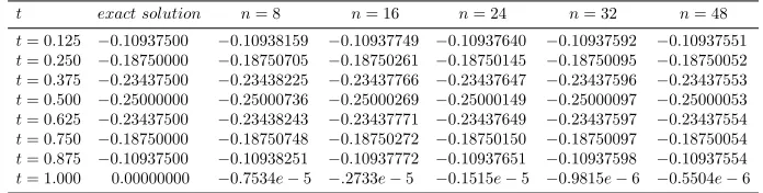
We apply the presented method on the (7.2) and the numerical results of the presented method are given in TABLE 1. We calculate its polynomial interpolation p(t) for (ti, ym(ti)), i = 1,2, . . . , n and k y(t)−p(t) k2 for different values of n, which are shown in TABLE2. It is obviously seen that the numerical results of our method are more accurate than of the results obtained from referred methods.
Table 1. Numerical results of Example 7.1
t exact solution n= 8 n= 16 n= 24 n= 32 n= 48
t= 0.125 −0.10937500 −0.10938159 −0.10937749 −0.10937640 −0.10937592 −0.10937551
t= 0.250 −0.18750000 −0.18750705 −0.18750261 −0.18750145 −0.18750095 −0.18750052
t= 0.375 −0.23437500 −0.23438225 −0.23437766 −0.23437647 −0.23437596 −0.23437553
t= 0.500 −0.25000000 −0.25000736 −0.25000269 −0.25000149 −0.25000097 −0.25000053
t= 0.625 −0.23437500 −0.23438243 −0.23437771 −0.23437649 −0.23437597 −0.23437554
t= 0.750 −0.18750000 −0.18750748 −0.18750272 −0.18750150 −0.18750097 −0.18750054
t= 0.875 −0.10937500 −0.10938251 −0.10937772 −0.10937651 −0.10937598 −0.10937554
t= 1.000 0.00000000 −0.7534e−5 −.2733e−5 −0.1515e−5 −0.9815e−6 −0.5504e−6
Table 2. Absolute errors of Example 7.1
ke8k2 ke12k2 ke16k2 ke24k2 ke32k2 ke48k2
P resented method 7.2850e−6 4.0478e−6 2.6559e−6 1.4716e−6 9.6072e−7 5.3383e−7
Ref.[35] − 1.0438e−4 − 2.6403e−5 − −
Ref.[41] 6.0313e−5 − 1.4484e−6 − 2.3374e−7 5.3445e−6
Ref.[36] − 7.7110e−4 − 2.0755e−5 − 5.3445e−6
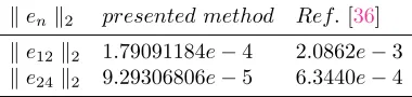
Example 7.2. As the second example, consider the following fractional Hammerstein integro-differential equation of Ref. [36]
D56y(t)−
Z 1
0
tes[y(s)]4ds= 3 Γ(1
6)
2t16 −431 91 t
13
with the initial conditiony(0) = 0 and exact solutiony(t) =t−t3. Using the fractional integral operator on both sides of the equation (7.3) and using of initial condition, yields
y(t) =t−t3− 1
Γ(56) 8928
55 t 11
6e−24264t 11
6
55
+ 1
Γ(56) Z t
0
Z 1
0
(t−τ)−61τ es[y(s)]4dsdτ. (7.4)
ky(t)−p(t)k2of the presented method and Ref. [36] are given in TABLE3.
Table 3. Numerical results of Example 7.2
ken k2 presented method Ref.[36]
ke12k2 1.79091184e−4 2.0862e−3
ke24k2 9.29306806e−5 6.3440e−4
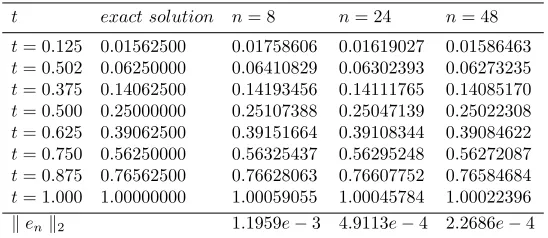
Example 7.3. Consider the following functional fractional Hammerstein integro-differential equation
D12y(t)−
Z 1
0
(t−s). (s−1) +sy(s 2)
ds= 8 3√πt
3 2 + 7
16t− 7
60, (7.5)
with the initial conditiony(0) = 0 and exact solutiony(t) =t2. Similar to the previous example, by using the fractional integral operator on both sides of the equation (7.5) and by using of initial condition, we obtain
y(t) =t2−√1 π
7t32 12 −
7√t
30 !
+ 1
Γ(12) Z t
0
Z 1
0
(t−τ)−21(τ−s). (s−1) +sy(s 2)
dsdτ. (7.6)
The numerical results of the presented method are given in TABLE4. Also,ky(t)− p(t)k2is reported in last line.
8. Conclusion
In this paper, we investigated on functional Hammerstein integro-differential equa-tions of fractional order. Here we also presented an approximate method to solve these equations. We proved convergence and stability of the method, too. At the end, we gave some numerical examples, which show the accuracy of the method.
Acknowledgment
Table 4. Numerical results of Example 7.3
t exact solution n= 8 n= 24 n= 48
t= 0.125 0.01562500 0.01758606 0.01619027 0.01586463 t= 0.502 0.06250000 0.06410829 0.06302393 0.06273235 t= 0.375 0.14062500 0.14193456 0.14111765 0.14085170 t= 0.500 0.25000000 0.25107388 0.25047139 0.25022308 t= 0.625 0.39062500 0.39151664 0.39108344 0.39084622 t= 0.750 0.56250000 0.56325437 0.56295248 0.56272087 t= 0.875 0.76562500 0.76628063 0.76607752 0.76584684 t= 1.000 1.00000000 1.00059055 1.00045784 1.00022396
kenk2 1.1959e−3 4.9113e−4 2.2686e−4
References
[1] J. H. Ahlberg, E. N. Nilson and J. L. Walsh, The Theory of splines and their applications, Academic Press, New York, London, 1967.
[2] F. Alhendi, W. Shammakh and H. Al-Badrani, Numerical solutions for quadratic integro-differential equations of fractional orders, Open Journal of Applied Sciences (OJAppS),7(2017), 157–170.
[3] S. Alkan and V. F. Hatipoglu,Approximate solutions of Volterra-Fredholm integro-differential equations of fractional order, Tbilisi Mathematical Journal,10(2) (2017), 1–13.
[4] A. Arikoglu and I. Ozkol,Solution of fractional integro-differential equations by using fractional differential transform method, Chaos, Solitons & Fractals,40(2) (2009), 521–529.
[5] T. M. Atanackovi´c, S. Pilipovi´c, B. Stankovi´c and D. Zorica, ,Fractional calculus with applica-tions in mechanics: vibraapplica-tions and diffusion processes, ISTE Ltd and John Wiley & Sons, Inc, Great Britain and the United States, 2014.
[6] T. M. Atanackovi´c, S. Pilipovi´c, B. Stankovi´c and D. Zorica,Fractional calculus with applica-tions in mechanics: wave propagation, impact and variational principles, ISTE Ltd and John Wiley & Sons, Inc, Great Britain and the United States, 2014.
[7] G. W. Bohannan,Analog fractional order controller in temperature and motor control applica-tions, Journal of Vibration and Control,14(2008), 1487–1498.
[8] R. Baillie,Long memory processes and fractional integration in econometrics, Journal of Econo-metrics,73(1996), 5–59.
[9] A. M. Bica, M. Curila and S. Curila,About a numerical method of successive interpolations for functional Hammerstein integral equations, Journal of Computational and Applied Mathemat-ics, 236(2012), 2005–2024.
[10] P. Cerone and S. Dragomir, Trapezoidal and midpoint-type rules from inequalities point of view, G. A. Anastassiou (Ed.), Hand book of Analytic Computational Methods in Applied Mathematics, Chapman Hall, CRC Press, Boca Raton, London, New York, Washington, DC, 2000.
[11] K. Diethelm,The analysis of fractional differential equations, Springer, 2004.
[12] I. Emiroglu, An approximation method for fractional integro-differential equations, Open Physics,13(2015), 370–376.
[13] A. A. Elbeleze, A. Klman and B. M. Taib,Approximate solution of integro-differential equation of fractional (arbitrary) order, Journal of King Saud University - Science,28(2016), 61–68. [14] A. A. Hamoud and K. P. Ghadle,Modified Laplace decomposition method for fractional
Volterra-Fredholm integro-differential equations, Journal of Mathematical Modeling,6(1) (2018), 91–104. [15] J. H. He,Nonlinear oscillation with fractional derivative and its applications, in: Proc.
Inter-national conference on vibrating engineering, China: Dalian, (1998), 288–291.
[17] L. Huang, X. F. Li, Y. Zhao and X. Y. Duan, Approximate solution of fractional integro-differential equations by Taylor expansion method, Computers & Mathematics with Applica-tions,62(3) (2011), 1127–1134.
[18] C. Iancu,On the cubic spline of interpolation, Seminar on functional analysis and numerical methods, Cluj-Napoca,4(1981), 52–71.
[19] C. Ionescu, A. Lopes, D. Copot, J. A. T. Machado and J. H. T. Bates ,The role of fractional calculus in modeling biological phenomena: A review, Communications in Nonlinear Science and Numerical Simulation,51(2017), 141–159.
[20] H. K. Jassim, The analytical solutions for Volterra integro-differential equations within lo-cal fractional operators by Yang-Laplace transform, Sahand Communications in Mathematical Analysis (SCMA),6(1) (2017), 69–76.
[21] S. Karimi Vanani and A. Aminataei, Operational Tau approximation for a general class of fractional integro-differential equations, Journal of Computational and Applied Mathematics,
30(3) (2011), 655–674.
[22] A. Kilicman and W. A. Ahmood,Solving multi-dimensional fractional integro-differential equa-tions with the initial and boundary condiequa-tions by using multi-dimensional Laplace Transform method, Tbilisi Mathematical Journal,10(1) (2017), 105–115.
[23] M. Kurulay and A. Secer,Variational iteration method for solving nonlinear fractional integro-differential equations, International Journal of Computer Science & Emerging Technologies (IJCSET),2(1) (2011), 18–20.
[24] P. Linz,Analytical numerical methods for Volterra equations, SIAM, Studies in Applied Math-ematics, 1985.
[25] A. M. S. Mahdy,Numerical studies for solving fractional integro-differential equations, Journal Of Ocean Engineering And Science (JOES),3(2018), 127–132.
[26] Z. Meng, L. Wang, H. Li and W. Zhang,Legendre wavelets method for solving fractional integro-differential equations, International Journal of Computer Mathematics,92(6) (2015), 1275–1291. [27] R. C. Mittal and R. Nigam,Solution of fractional integro-differential equations by Adomian de-composition method, International Journal of Applied Mathematics and Mechanics,4(2) (2008), 87–94.
[28] S. Momani and M. Noor, Numerical methods for fourth order fractional integro-differential equations, Applied Mathematics and Computation,182(2006), 754–760.
[29] Y. Nawaz,Variational iteration method and homotopy perturbation method for fourth order fractional integro-differential equations, Computers and Mathematics with Applications, 61
(2011), 2330–2341.
[30] D. Nazari and S. Shahmorad, Application of the fractional differential transform method to fractional-order integro-differential equations with nonlocal boundary conditions, Journal of Computational and Applied Mathematics, 234(3) (2010), pp. 883-891.
[31] K. Oldham,Fractional differential equations in electrochemistry, Advances in Engineering Soft-ware,41(2010), 9–17.
[32] I. Podlubny,Fractional differential equations, Mathematics in Science and Engineering, Aca-demic Press, San Diego, 1999.
[33] S. S. Ray,Analytical solution for the space fractional diffusion equation by two-step Adomian decomposition method, Communications in Nonlinear Science and Numerical Simulation, 14
(2009), 1295–1306.
[34] L. J. Rong and P. Chang,Jacobi wavelet operational matrix of fractional integration for solving fractional integro-differential equation, Journal of Physics: Conference Series,693(2016), 1–14. [35] H. Saeedi, Application of Haar wavelets in solving nonlinear fractional Fredholm integro-differential equations, Journal of Mahani Mathematical Research Center (JMMRC),2(1) (2013), 15–28.
[37] H. Saeedi and F. Samimi,Hes homotopy perturbation method for nonlinear Fredholm integro-differential equations of fractional order, International Journal of Engineering Research and Applications (IJERA),2(5) (2010), 052–056.
[38] Y. Wang and L. Zhu,Solving nonlinear Volterra integro-differential equations of fractional order by using Euler wavelet method, Advances in Difference Equations,27(2017), 1–16.
[39] J. Wang, T. Z. Xu, Y. Q.Wei and J. Q. Xie,Numerical simulation for coupled systems of non-linear fractional order integro-differential equations via wavelets method, Applied Mathematics and Computation,324(2018), 36–50.
[40] A. Youse, T. Mahdavi-Rad and S. G. Shaei, A quadrature Tau method for solving fractional integro-differential equations in the Caputo sense, International Journal of Mathematics and Computer Science,15(2015), 97–107.