81 *
Corresponding author
Email address:[email protected]
Dissimilar friction stir lap welding of Al-Mg to CuZn34: Application
of grey relational analysis for optimizing process parameters
Saman Khalilpourazarya*, Reza Abdi Behnagha,b, Ramezanali Mahdavinejadb and Nasib Payama
a
Department of Mechanical Engineering, Urmia University of Technology, Urmia, Iran
b
School of Mechanical Engineering, College of Engineering, University of Tehran, Tehran, Iran
Article info: Abstract
This study focused on the optimization of Al—Mg to CuZn34 friction stir lap welding (FSLW) process for optimal combination of rotational and traverse speeds in order to yield favorable fracture load using Grey relational analysis (GRA). First, the degree of freedom was calculated for the system. Then, the experiments based on the target values and number of considered levels, corresponding orthogonal array, Grey relational coefficient and Grey relational grade were performed. In the next step, Grey relational graph of each level was sketched. The performed graph and analysis of Grey results proved the impact of rotational speed and traverse speed on fracture load of resultant joints. Finally, the optimum amount of each parameter for better strength of the welds was obtained. This study showed feasibility of the application of Grey relational analysis for achieving dissimilar friction stir lap welds with the highest quality.
Received: 02/07/2013 Accepted: 09/11/2013
Online: 11/09/2014
Keywords:
FSLW, Dissimilar, Optimization,
Grey relational analysis.
1. Introduction
Development of sound joints between dissimilar materials is of great importance in many emerging applications including chemical, nuclear, aerospace, transportation, power generation and electronics industries [1]. Joining dissimilar materials by conventional fusion welding is difficult for two reasons: (i) poor weldability arises due to different chemical, mechanical and thermal properties of the welded materials and (ii) hard and brittle intermetallic compounds (IMC) are usually formed at the weld interface. Friction stir welding (FSW) is a technique invented by Welding Institute (1991) for joining aluminium alloys [2]. This technique results in low
distortion and high joint strength in comparison to other techniques and is capable of joining all aluminium alloys including dissimilar ones [3]. It uses a non-consumable rotating tool to generate frictional heat and deformation at the welding zone, leading to the formation of a joint while materials are still in solid state [4]. At the joint, the material is frictionally heated to the temperatures, at which it is easily plasticized.
82
applications. Aluminums and its alloys are characterized by relatively low density, high electrical and thermal conductivities and resistance to corrosion in some common environments [6]. Aluminum makes brass stronger and more corrosion resistant and joining of these two metals can be used in power plants, heat exchangers, radiators and electrical applications. In the previous study of the present authors, feasibility of friction stir lap welding (FSLW) of dissimilar joints of an aluminum plate to a brass one was investigated. It was reported that the nature of the weldment materials as well as FSLW parameters such as tool rotational and traverse speeds and joint design had a significant influence on the weld quality and consequently determining optimum FSW conditions is very important [7].
Taguchi method is very popular for solving optimization problems in the field of production engineering [8]. However, traditional Taguchi method cannot solve multi-objective optimization problem. To overcome this shortcoming, Taguchi method coupled with Grey relational analysis has a wide area of application in manufacturing processes. This approach can solve multi-response optimization problem simultaneously [9]. Planning the experiments through Taguchi orthogonal array has been used quite successfully in process optimization in several attempts. Recently, Aydin et al. studied friction stir welding process conditions of 1050 aluminum alloy in order to get the highest strength of the welds [9]. This study applied Grey relational analysis (GRA) to plan the experiments on Al-Mg to CuZn34 friction stir lap welding process. Two controlling factors including rotational speed (N) and welding speed (ν) were selected. Grey relational analysis was then applied to examine how the welding process factors influenced lap shear fracture load (LSFL) as the most important factor of mechanical properties.
2. Levels of factors in the experiment
Grey analysis method was introduced for the first time in 1982 [10]. According to this theory, the method, owing to lack of difficulties and infeasibility of other methods, can be
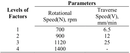
applied for the systems with multiple objectives [10]. In Grey analysis, each test has input parameters divided to levels according to the application conditions or effectiveness. In this paper, the experiments were performed for two parameters (rotational speed and traverse speed) at four different levels (Table 1). In the next step, the machine set up was done via all the data provided in Table 1.
Table 1. Process parameters and related levels.
Levels of Factors
Parameters
Rotational Speed(N), rpm
Traverse Speed(V),
mm/min
1 700 6.5
2 900 12
3 1120 25
4 1400 -
3. Orthogonal array
To select an appropriate orthogonal array for the experiments, the total degrees of freedom need to be computed. The degrees of freedom for the orthogonal array should be greater than or equal to those for the process parameters. These arrays are
m
n
matrixes with the rows as the number of tests and columns as the input parameters. The matrix is built in the way that repeating tests are identified while the experiments are carried out to satisfy the minimum number of tests such that the final target can be achieved. The total degree of freedom for the proposed system is calculated as follows [10]:(1)
FD =1+(Degree of Freedom×level)
Then, the obtained value for degree of freedom was:
6 ) 2 3 (
1
FD
83 Table 2. Orthogonal array of the experimental runs
and results.
Run
Parameters Experimental results
N V Failure load
(N)
1 1 1 4321
2 1 2 4121
3 1 3 3752
4 2 1 4829
5 2 2 4532
6 2 3 3896
7 3 1 5432
8 3 2 4931
9 3 3 4178
10 4 1 4572
11 4 2 3421
12 4 3 3298
4. Experimental analysis and test results
4.1. Details of experimental procedure
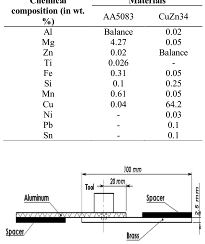
Two dissimilar sheets were used in the FSW process carried out in the present work: a 5083 aluminum alloy sheet and a brass sheet. The sheets were 2.5 mm thick and their chemical compositions are given in Table 3.
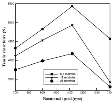
The sheets were cut and machined into rectangular welding samples, 200 mm long and 100 mm wide, which were longitudinally lap-welded using a conventional milling machine. The aluminum alloy sheet was placed on the brass alloy sheet. Then, a rotating tool was plunged from the aluminum alloy surface into the surface of brass. It was reported that a better FSW configuration was acquired when the welding tool was essentially plunged into the softer material [11]. The penetration depth of the tool into a lower material was about 1 mm. Relative position of aluminum alloy and brass is shown in Fig. 1.
The top sheet (Al) had the retreating side near the edge; i.e. all the welds were configured in such a way that the retreating side of the tool was always located near the top sheet edge (RNE). The welding tool used in the FSW process was made of 2436 steel alloy, which
encompassed a concave shoulder with diameter of 20 mm and a non-threaded cylindrical pin with length and diameter of 3.5 and 6 mm, respectively. Tilt angle of the rotating tool with respect to the z-axis of the milling machine was about 1.5 degrees for all the samples. The lap joining process was performed via FSW at the tool rotational speeds of 700, 900, 1120 and 1400 rpm and traverse speeds of 6.5, 12 and 25 mm/min. In order to characterize mechanical properties of the joint under various welding conditions, a set of lap shear tests was carried out according to ISO 12996 standard [12]. The failure load was recorded for each sample. Shape of the test specimen was rectangular and width of each specimen was 15 mm.
Table 3. Chemical composition of welded materials.
Chemical composition (in wt.
%)
Materials
AA5083 CuZn34
Al Balance 0.02
Mg 4.27 0.05
Zn 0.02 Balance
Ti 0.026 -
Fe 0.31 0.05
Si 0.1 0.25
Mn 0.61 0.05
Cu 0.04 64.2
Ni - 0.03
Pb - 0.1
Sn - 0.1
Fig. 1. A schematic presentation of the relative position of aluminum alloy, brass and the tool.
4.2. Effect of process parameters on failure loads of lap shear tests
cross-84
sections of the joints produced in various welding conditions are shown in Table 4. Table 4. Typical micrographs for the macrostructure of cross-sections of FSW joints.
Welding conditions
Macrograph of joint
structure Observation
Rotational speed (rpm):
700
Name of defect:
Tunnel
Welding speed (mm/min):
12.5
Rotational speed (rpm):
900
Name of defect:
Defect free Welding
speed (mm/min):
6.5
Rotational speed (rpm):
1120
Name of defect:
Defect free Welding
speed (mm/min):
6.5
Rotational speed (rpm):
1400
Name of defect:
Defect free Welding
speed (mm/min):
6.5
Rotational speed (rpm):
1400
Name of defect:
Defect free Welding
speed (mm/min):
12
Rotational speed (rpm):
1400
Name of defect:
Pin hole Welding
speed (mm/min):
25
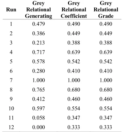
Lap joints might be primarily loaded either by peel or in shear. In this study, strength of the lap joints which were nominally loaded in the overlap shear was examined. Failure loads of the joints in the lap shear tests are given in Fig. 2.
Fracture loads of all the joints were found to be lower than those of the base materials and ranged from 3.3 ± 0.3 kN to 5.4 ± 0.4 kN. As illustrated in Fig. 2, increasing rotational speed of the tool at constant traverse speeds of 6.5, 12 and 25 mm/min resulted in increase of the failure load to maximum and then a decrease in failure load appeared.
Fig. 2. Effect of rotational and traverse speeds on lap shear fracture load.
Maximum load was investigated for the traverse and rotational speeds of 6.5 mm/min and 1120 rpm, respectively. The two important parameters affecting the FSW were rotational speed and traverse speed. Rotation of the tool led to mixing and stirring the materials around the rotational pin. In addition, tool traverse displaced the stirred material from the front to the back of the pin. In FSW processes, higher rotational speeds or lower welding speeds led to more heat input, which in turn provided better conditions for diffusion reactions of Al and CuZn34 and consequently resulted in a thick weld zone (fine grained zone). In addition, according to the results of lap shear tests, fracture in the entire weld specimens occurred in the HAZ region, except the specimens welded with tool rotational speed of 1400 rpm. Shear load of the joint was probably affected by two factors: the amount of brittle and hard intermetallic compounds and ‘cold weld’ condition which was performed at low rotational and medium or high translational speed. By increasing rotational speed (or decreasing welding speed) of the tool, the frictional heat generation increased and led to more intense stirring and mixing of the materials and consequently increasing size of the fine grained zone (nugget). Therefore, mechanical strength of the joint was improved with increasing the rotational speed or reducing the traverse speed. Further increase of rotational 1 mm
RS AS
1 mm RS AS
1 mm RS AS
1 mm
AS RS
1 mm RS AS
85 speed resulted in a large amount of intermetallic
compounds (larger dark area) at the interface between aluminium and copper; so, the shear load was decreased [13]. The reason for the increase in the amount of intermetallic compounds was that higher rotational speed raised higher temperature at the interface because the formation process of intermetallic compounds was thermally activated. With increasing the temperature, nucleation and growth of these compounds were accelerated [13].
5. Application of grey relational analysis for FSLW parametric optimization
Using Grey analysis, the problem with multiple objectives was changed to the problem with one objective, which led to easier analyses and inferences of data. After normalizing the data which was done in the stage of generating Grey relational to obtain Grey relational coefficient and Grey relational grade, the final decision from the plotted Grey graph could be made. 5.1.Grey relational generating
Due to the different restrictions and amounts associated with the optimization parameters, a rather challenging comparison is expected. Hence, normalization is necessary to achieve a valid comparison between the parameters. Equations (2-4) introduce the relations of different possibilities with the normalization process. If the target value of original sequence is infinite, a characteristic of ‘‘the-larger-the-better’’ can be expected. The original sequence can be normalized as follows [14]:
(2) , ) ( min ) ( max ) ( min ) ( 1 ) ( 0 0 0 0 * k X k X k X k X k X i i i i i
Since smaller values are desired, the original sequence can be normalized as follows:
(3) , ) ( min ) ( max ) ( ) ( max 1 ) ( 0 0 0 0 * k X k X k X k X k X i i i i i
In case there is a definite target value to be achieved, the original sequence can be normalized as follows:
(4) , ) ( max ) ( 1 ) ( 0 0 0 0 * X k X X k X k X i i i
where
X
i*(
k
)
is value after Grey relational generation (data pre-processing),max
X
i0(
k
)
is the largest value ofX
i0(
k
)
,min
X
i0(
k
)
is the smallest value ofX
i0(
k
)
and0
X
is the desired value [15].X
i*(
k
)
is the result of Grey analysis for the ith response in the kth test while)
(
k
X
i represents the parameter value before the analysis [16]. Eq. (2) can be used for finding maximum value of the failure load of the lap shear tests.5.2.Grey relational coefficient
Grey Relational Coefficient has a value between zero and one, and indicates the distance from the ideal value. Grey Relational Coefficient is calculated using the following formula [16]: (5) , ) ( ) ( max 0 max min k k i i
Where,min represents minimum deviation of data values, maxis maximum deviation of data values,0i(k)shows deviation value for the reference data, and i(k) is grey coefficient. Each parameter in Eq. (5) is calculated separately using the following equations [17]:
(6) , ) ( ) ( )
( 0* *
0i k X k Xi k (7) , ) ( ) ( max
max 0* *
max X k Xi k (8) , ) ( ) ( min
min 0* *
min X k Xi k
86
5.3.Grey relational grade
Grey relational grade is a parameter obtained after Grey relational coefficient. This parameter is determined using Eq. (9), when effects of all the parameters are assumed to be equal [19]:
(9)
, ) ( 1
1
m
k i
i k
m
where
ijis Grey relational coefficient and
i is Grey relational grade. Table 5 lists the related Grey relational grade for each Grey relational coefficient.5.4.Grey relational grade for each level
Equations (10 and 11) can be used to determine Grey relational grade for each level. It is obvious that Grey relational grade for each level is the average amount of all grades [19]:
(10)
, 1
1
k
i i
k
A
(11)
,
n m k
where
A
indicates Grey grade for each level,k is a constant coefficient, m represents the number of tests and n is the number of levels. Table 6 includes a column listing Max-Min values for Grey grade data obtained from the maximum and minimum values of Grey grade for each level. These values indicate robustness of each parameter. When it is high for a parameter, the corresponding parameter is unstable and vice versa [20].
6. Grey relational graph
Grey relational graph is graph of the table containing levels and Grey relational grade for each level. This graph is easily drawn by connecting the table points to each other. In this study, Grey graph for each level was drawn according to the obtained tables. Also, two graphs were integrated into one for better comparison (see Fig. 3). The amount of slope in Fig. 3 indicates sensitivity of that parameter (e.g. as slope decreased, effectiveness of the parameter decreased as well).
Table 5. Grey relational grade and Grey relational coefficient.
Run
Grey Relational Generating
Grey Relational Coefficient
Grey Relational
Grade
1 0.479 0.490 0.490
2 0.386 0.449 0.449
3 0.213 0.388 0.388
4 0.717 0.639 0.639
5 0.578 0.542 0.542
6 0.280 0.410 0.410
7 1.000 1.000 1.000
8 0.765 0.680 0.680
9 0.412 0.460 0.460
10 0.597 0.554 0.554
11 0.058 0.347 0.347
12 0.000 0.333 0.333
Table 6. Grey relational grade for each level.
Parameters Levels Max-Min
1 2 3 4
Rotational
speed (rpm) 0.44 0.53 0.71 0.41 0.302
Traverse speed (mm/min)
0.67 0.5 0.4 0.273
7. Results
87 Fig. 3. Grey relational graph of the process.
Table 7. Optimum values for all the parameters.
Parameters Optimum condition
Optimum test
Traverse speed
(mm/min) 6.5 6.5
Rotational speed
(rpm) 1120 1120
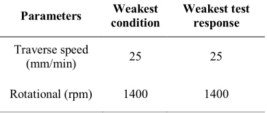
Table 8. Worst values of the parameters.
Parameters Weakest condition
Weakest test response
Traverse speed
(mm/min) 25 25
Rotational (rpm) 1400 1400
8. Conclusions
Grey relational analysis (GRA) is one of the optimization methods under a limited number of experimental runs. In this study, rotational speed and traverse speed were considered internal parameters for optimizing friction stir lap welding of 5083 aluminum alloy to CuZn34 using Grey relational analysis. Also, the corresponding
L
12orthogonal array was selected prior to investigating degree of freedom for the system and the number of the levels for the tests. Following Grey relational generation and calculating Grey relational coefficient and grade, the Grey graph was drawn based on the Grey grade for each level. Finally, according to the Grey graph, the optimal amount of eachparameter for maximum lap shear load was exploited. It was shown that:
1- According to the Grey graph in Fig. 3 for each traverse speed, when the rotational speed was enhanced from 700 rpm to 1120 rpm, the test results improved.
2- Increasing rotational speed up to 1120 rpm (under similar traverse speeds) led to poor results.
3- Increasing traverse speed from 6.5 mm/min to 25 mm/min led to decreasing failure load of the joints.
4- Grey relational analysis had drastic capability in optimizing mechanical properties of dissimilar friction stir lap welded AA5083 to CuZn34 rolled plates.
References
[1] R. Zettler, S. Lomolino, J. F. Dos Santos, T. Donath, F. Beckmann, T. Lippman and D. Lohwasser, “Effect of Tool Geometry and Process Parameters on Material Flow in FSW of an AA 2024-T351 Alloy”, Weld in World, Vol. 49, No. (3-4), pp. 41-46, (2005).
[2] P. Cavaliere and A. Squillace, “Effect of welding parameters on mechanical and microstructural properties of dissimilar AA6082-AA2024 joints produced by Friction Stir Welding”, Mater Sci forum, Vol. 519, No. 2, pp. 1163-1168, (2006). [3] R. S. Mishra and Z. Y. Ma,“Friction Stir
Welding and Processing”, Mater SciEng R., Vol. 50, No. 3, pp.1-78, (2005).
[4] V. Soundararajan, E. Yarrapareddy and R. Kovacevic,“Investigation of Friction Stir Lap Welding of Aluminum Alloys
AA5182 and AA6022”, J.
Mater Eng. Perform, Vol. 16, No. 4, pp. 477-484, (2006).
[5] L. Dubourg, A. Merati and M. Jahazi, “Process Optimization and Mechanical Properties of Friction Stir Lap Welds of 7075-T6 Stringers on 2024-T3 Skin”, Mater. Des., Vol. 31, No. 7, pp. 3324-3330, (2010).
88
[7] M. Movahedi, A. H. Kokabi, S. M. SeyedReihani and H. Najafi, “Effect of tool travel and rotation speeds on weld zone defects and joint strength of aluminium steel lap joints made by friction stir welding”, Science and Technology of Welding and Joining, Vol. 17, No. 2, pp. 162-167, (2012).
[8] M. Akbari, R. AbdiBehnag and A. Dadavand,“Effect of Materials Position on Friction Stir Lap Welding of Al to Cu”, Sci Technol Weld Join,Vol. 17, No. 7, pp. 581-588, (2012).
[9] A. Esmaeili, M. K. BesharatiGivi and H. R. ZareieRajani, “A Metallurgical and Mechanical Study on Dissimilar Friction Stir Welding of Aluminum 1050 to Brass (CuZn30)”,Mater SciEng A, Vol. 528, No. (22-23), pp. 7093-7102, (2011). [10] C. L. Lin, “Use of the Taguchi Method
and Grey Relational Analysis to Optimize Turning Operations with Multiple Performance Characteristics”, J. Mater Process Technol, Vol. 19, No. 2, pp. 209-220, (2004).
[11] W. B. Lee, M. Schmuecker, U. A. Mercardo, G. , Biallas and S. B. Jung, “Interfacial Reaction in Steel-Aluminum Joints Made by Friction Stir Welding”, ScriptaMaterialia, Vol. 55, No. 4, pp. 355-358, (2006).
[12] DIN EN ISO 2768-1:2013. Mechanical joining - Destructive testing of joints- Specimen dimensions and test procedure for tensile shear testing of single joints. [13] M. Akbari and R. AbdiBehnagh,
“Dissimilar Friction-Stir Lap Joining of 5083 Aluminum Alloy to CuZn34 Brass”, Metall Mater Trans B,Vol. 43, No. 5, pp.1177-1186, (2012).
[14] B. C. Routara, B. K. Nanda, A. K. Sahoo, D. N. Thato and B. B. Nayak,
“Optimization of Multiple Performance Characteristics in Abrasive Jet Machining Using Grey Relational Analysis”, Int J. Manufact. Technol. Manag, Vol. 24, No. (1-3), pp. 4-22, (2011).
[15] M. Nalbant, H. Gokkaya and G. Sur, “Application of Taguchi Method in the Optimization of Cutting Parameters for Surface Roughness in Turning”, J. Mater Process Technol,Vol. 28, No. 4, pp. 1379-1385, (2007).
[16] L. K. Pan, C. C. Wang, S. L. Wei and H. F. Sher,“Optimizing Multiple Quality Characteristics via Taguchi Method-Based Grey Analysis”, J. Mater Process Technol,Vol. 182,No. (1-3), pp. 107-116, (2007).
[17] H. S. Lu, C. K. Chang, N. C. Hwang and C. T. Chung, “Grey Relational Analysis Coupled with Principal Component Analysis for Optimization Design of the Cutting Parameters in High-Speed End Milling”, J. Mater Process Technol., Vol. 209, No. 8, pp.3808-3817, (2009).
[18] J. Kopac and P. Krajnik, “Robust Design of Flank Milling Parameters Based on Grey-Taguchi Method”, J. Mater Process Technol,Vol. 191, No. (1-3), pp. 400-403, (2007).
[19] J. L. Lin and Y. S. Tarng, “Optimization of the Multi-Response Process by the Taguchi Method with Grey Relational Analysis”, J. Grey Sys., Vol. 4, No. 4, pp. 355- 370, (1998).