The Relation between Implied Volatility Index and Crude Oil Prices

The Relation between Implied Volatility Index and Crude Oil Prices

Imlak Shaikh

Department of Accounting and Finance Management Development Institute Gurgaon Haryana 122007, India

E-mail. [email protected]; [email protected]

http://dx.doi.org/10.5755/j01.ee.30.5.21611

Crude oil is a global commodity traded across the world market. The prices of the commodity over an extended period for crude oil have been analyzed using daily prices of crude oil futures and the implied volatility index (OVX). This paper aims to find the predictability of various parameters on the basis of time using neural network and quantile regression methods. Several estimates have been shown based on Barone, Adesi, and Whaley’s (BAW) model of neural network. Estimation parameters include opening, closing, highest and lowest price of the commodity and volumes traded for a given commodity on each trading day. The neural network estimates explain that future prices of the WTI/USO can be predicted with minimal error, and similar can be used to predict future volatility. The quantile regression results suggest that crude oil prices and OVX are strongly associated. The asymmetric association between the WTI/USO and OVX explains that the volatility feedback effect holds good for the OVX market. Bai and Perron least squares estimate evidence of the presence of a break in the time series. The main results uncover several interesting facts that implied volatility tends to remain calm during the global financial crises and higher throughout the post crisis period. The empirical outcome on the OVX market provides some practical implications for the trader and investor, in which oil futures can serve better to hedge the crude price volatility. The crude oil producer can short hedge enough through volatility futures and options to maintain the future quantity of crude to be produced.

Keywords: Crude oil price; Chicago Board of Options Exchange; Implied Volatility; Oil Volatility Index; West Texas Intermediate; United States Oil Fund; Exchange Traded Fund.

Introduction

Crude oil is a global commodity traded across the world market. According to the U.S. Energy Information Administration Department, there are mainly five prices of spot crude oil traded globally, including the West Texas Intermediate, Brent, Mars, Tapis, and Dubai. It consists of various categories produced, and the value tends to change significantly over the period. For example, crude oil prices were spiked by about $20 per barrel in 1999 to $150 per barrel in 2016, and the prices remained highly variable during the period 2010–2016 (e.g., see EIA, 2019). Because crude oil is a highly demanded product from large economies such as the U.S., China, Japan and India, and with a limited supply from few countries such as the Middle East region and Russia, crude oil prices on different counter markets are greatly influenced by several economic, financial, geopolitical, geological and weather factors. These important factors have a considerable impact on the future demand and supply of crude, and traders’ ambiguity results in higher volatility of crude prices. The short run dynamics explain crude demand and supply elasticity toward price inelasticity. Hence, price fluctuations in the short-run may have a negligible impact on the petroleum and energy market, though large ups and downs may severely disrupt the entire market system (e.g., see Nakanishi & Komiyama, 2006). The recent price fluctuations were mainly due to political issues triggered in the Middle East region and the Arab oil embargo (e.g., Narayan & Narayan, 2007; Arouri et al., 2011).

USO fund is an ETF security intended to track oscillations in crude oil prices. By holding futures contracts and cash in the near term, the performance of the fund is envisioned to replicate, as closely as possible, the spot price of WTI, Sweet crude oil, and adjusting USO expenses.

The work aims to find the predictability of various parameters based on the time using the neural network and quantile regression. The assessment has been done considering the Barone, Adesi, and Whaley (BAW) model of neural network. Such parameters are opening, closing, highest, lowest price of the commodity and volumes traded of the commodity for each trading day. The parameters are the basic ones that define a complete transaction for the commodity. The implied volatility is the forward looking measure of future stock market volatility. It is the volatility to be realized for the remaining life of the option. S&P 500 and OEX options’ based volatility index for the near term first time expressed as VIX and VXO. VIX is commonly known as the investor’s ‘fear gauge index’; it is the expectation of future realized volatility. VIX as the stock market barometer of future volatility, e.g., VXN, VXD, VVIX, VXJ, VKOSPI, NVIX, TVIX, AVIX, GRIV, VX1, etc., is now available for most of the stock exchanges over the world. It has been observed that implied volatility has significant forecasting ability to predict future market volatility (e.g., Shaikh, 2018). OVX gauges the future crude oil market volatility; henceforth, it is important to study the relationship between OVX and WTI/USO futures returns. The literature analysis presented in the next section evidence a significant negative correlation between volatility and stock returns. Besides, the relation is asymmetric i.e. the negative returns show a larger impact than the positive returns.

Remaining work is organized as follows: Section “Literature analysis” presents review of earlier studies in the crude oil market; Section “Data and methodology” provides data description and summary statistics, followed by empirical method employed in the study and results and discussion, and Section “Conclusion” ends with the summary and conclusion.

Literature Analysis

The commodity traders are intensely concerned about analyzing the oil price volatility. Earlier studies (e.g., Fong & Sec, 2002; Martens & Zein, 2004; Agnolucci, 2009; Rafiq et al., 2009; Wei et al., 2010; Haugom et al., 2014 and Ghassan & AlHajhoj, 2016) on oil price volatility using GARCH type framework are having one period ahead forecasts horizon. Hence, the motivation of the study is to forecast oil prices and compare the impact of WTI/USO futures’ price returns on the expected volatility (OVX).

Unlike recent studies (e.g., Giot, 2005; Dowling & Muthuswamy, 2005; Ederington & Guan, 2010 and Frijns et al., 2010a, 2010b) has described asymmetric relation between stock returns and volatility. Indeed, the asymmetric relation of OVX and WTI/USO has not been explored. The literature institutes that the volatility of stock markets appears to be higher following negative returns rather than positive return shocks. Similarly, VIX based studies (e.g., Bates, 2000; Poteshman, 2001 & Dennis et al., 2006;

Shaikh, 2018) also confirm the asymmetric relation between stock returns and implied volatility. Moreover, Fleming et al. (1995), Whaley (2000), Low (2004) and Bollerslev and Zhou (2006) enlightens that negative and positive return shocks do have an asymmetric impact on future stock market volatility. They also report that implied volatility decreases sharply for large positive returns shocks.

There are two fundamental hypotheses, namely volatility feedback effects and leverage effects that govern asymmetric relation between returns and volatility. The volatility feedback hypothesis (e.g., French et al., 1987; Campbell & Hentschel, 1992) describes that an expected increase in the asset’s volatility causes an increase in the risk premium of assets. Similarly, the leverage effects (e.g., Black, 1976 & Christie, 1982) clarifies that decay in the stock prices causes a deterioration in the value of the firm. And consequently, it leads to an enlarged risk of the firm’s stock prices. Henceforth, Schwert (1989,1990) and Fleming et al. (1995) attempt to first explain an asymmetric relationship between stock returns and volatility and find that this relation good hold due to ‘volatility feedback effects’ and ‘leverage effects’. The crude oil is a global commodity- international financial institutions formulate their trading strategies (e.g., Warin and Sanger, 2018) in such a way to hedge oil price risk.

Amano and Norden (1998) first to examine the effects of oil prices on the US exchange rate. They find that the exchange rate and oil prices are linked over the post Britton wood period. The exchange rate shocks imply that energy prices hold important information to explain the behavior of the real exchange rate. Fong and Sec (2002) examine the crude oil futures prices using a Markov switching model. They find the presence of regime shift in time series, and it dominates the GARCH effects. Out of sample forecast and regime switching model explain the evolution of volatility in the futures market. Agnolucci (2009) compares the volatility forecast of the WTI futures market based on the GARCH type model and implied volatility where forecasts are attained by reversing the option pricing model. Moreover, the author evaluates the asymmetric effects and WTI futures market volatility using a GARCH model. Wei et al. (2010) extend their work in GARCH class models. They find that a nonlinear model is more superior to the linear model to forecast the five and twenty day volatility of the market.

find significant oil price co-movement with major economic activities in a cointegrating framework. Jouini (2013) examines returns and volatility for Saudi Arabia and finds spillover effects are unidirectional from oil to another market. Moreover, volatility transmission is present from oil to the stock sector.

Martens and Zein (2004) first evaluate the financial market volatility based on the implied volatility and historical returns across different financial assets, including commodities. Volatility forecast based on historical returns were dominating the options’ based implied volatility in high frequency data framework. Liu et al. (2013) investigate the co-movement between OVX and other market based volatility indices. Such as VIX(Stock), EVZ(Euro) and GVZ(Gold). They find no strong association between these indices and suggest that interior and exterior uncertainty shocks effects on OVX and found to be transient and positive. Aboura and Chevallier (2013) bring some new shreds of evidence to explain the relation between oil price volatility and oil prices based on the OVX and WTI prices. They find leverage and feedback effects good hold for this market and suggest trading strategy using F&O on the OVX volatility index. Haugom et al. (2014) analyze the information contained in OVX and forecasting historical returns based on realized volatility using WTI futures. The out of sample forecast shows that realized volatility along with implied volatility measure is the best model for forecasting.

Al-Abri (2013) empirically analyze the response of macroeconomic indicators concerning exchange rate regimes for the nine oil importing economy. The results support Friedman’s hypothesis, and causality tests advocate a feedback effect in terms of exchange rates and inflation rates in addition to oil price shocks. Conrad et al. (2014) employ the DCC-MIDAS model to analyze the long run correlation between crude price and stock price returns for the US macroeconomy. It is evident from the analysis that countercyclical behavior exists in long-run correlations. Ajmi et al. (2015) examine the relationship between crude oil price and consumer price nexus in South Africa. Authors employ asymmetric causality approach and find the short run causal relationship between oil price and price level. Christoffersen and Pan (2017) analyzes the oil price volatility risk and expected stock returns. They find oil price volatility risk carries a significant risk-premiums per month and also report that a rise in oil price ambiguity causes the performance of financial intermediaries.

Awartani et al. (2016) and Maghyereh et al. (2016) investigates implied volatility indices, equity market, and commodities and their linkages. Awartani et al. (2016) examine eleven major volatility indices and connectedness between crude oil prices and equity markets. They find uniform outcomes across countries and connectedness between the oil price and equity market. It is set up by bi-directional information spillovers among the two markets. Maghyereh et al. (2016) find significant volatility transmission from crude oil price market to equities but diminutive transmission to commodities. Galyfianakis et al. (2017) investigate the effects of commodities and financial markets on crude oil prices. They analyze the endogenous casual relationship using the VAR framework and find a close linkage between oil price shock and macroeconomic

activity. Zhu et al. (2017) examine the spillover effects between crude oil price and natural-gas markets using rolling VAR and frequency domain Granger causality tests. They find significant casualty relations from the oil market to gas in ‘put options’ based select samples.

Chen and Zou (2015) examine the CBOE OVX and crude oil price in a time-varying coefficient by employing the Kalman filter framework. Unlike a strong negative correlation between VIX and SPX, they find a weak negative asymmetric relationship between OVX and oil price returns. Dutta (2017) studies the oil price uncertainty and clean energy stock returns by calculating the realized volatility of alternative energy sector equity returns. He finds that OVX provides additional information to forecast the energy sector returns volatility than the historical returns of equity. Luo and Qin (2017) examine the impact of oil price volatility/shocks on the Chinese stock market. The empirical outcome shows that oil price shocks affect positively to the Chinese stock market. Moreover, on the comparison of the effects of realized volatility and OVX on the stock returns, OVX shocks are more effective.

Recent studies in developed and emerging markets (e.g., Martens & Zein, 2004; Lin et al., 2013; Aboura & Chevallier, 2013; Haugom et al., 2014; Chen & Zou, 2015; Maghyereh et al., 2016; Dutta, 2017 and Luo & Qin, 2017) specifically they examine the expected oil price volatility in terms of OVX. They analyze the relationship between OVX and WTI futures returns and spillover effects of crude oil price in developed and other emerging market based volatility indices. Moreover, e.g., Soltes and Harcarikova (2017) take the opportunity to propose new financial instruments in the oil market using a new barrier outperformance certificate to develop new barrier options. Furthermore, Bein (2017) explores the time varying co-movement between stock and oil market, and Kregzde (2018) develop the Wavelets based model to analyze the co-movement of stock returns in the European market. Hence, the present work is the extension of the previous work for the longer time series of OVX. The novel aspect of the current study is it encompasses USO-ETF prices to examine the behavior expected oil price volatility (OVX).

Data and Methodology

Description of Data

variable that cannot be directly observed. By equating market option price 𝐶_𝑡(𝑇−𝑡) and solving the 𝐶_𝑡(𝑇−𝑡)= BS{ 𝑇 − 𝑡,𝑆(𝑡),𝐾, 𝑅𝑓,

𝜎

2

},

the resulting value is known as implied volatility. By inverting the Black Scholes model, implied volatility can be obtained for the reaming life of the observed traded option. The daily prices of OVX, WTI, and USO, considered for the period 05/2007 to 05/2016. The USO is an ETF security build to track crude oil prices. The broad aim of holding the USO fund is to reflect the performance of WTI spot price, Sweet crude oil price, less USO-ETF expenses. Hence, OVX is the first commodity based implied volatility index. USO based options price reflect the true investor sentiment trading into WTI light and Sweet crude oil. The USO fund is held in cash and cash equivalents, government securities with two years of maturities. Hence, the USO fund offers commodity risk exposure without trading into commodity futures.

ANN and Forecasting

ANN is a computational method that has proficiency similar to the neuron network in the human brain. The architecture of the human brain is the main pattern behind this technology, and it uses many natural processing elements working in parallel to get high computational rates. The forecast available from neural networks outperforms general volatility forecasts, and forecast errors are not too divergent from realized volatility based on daily returns. The conventional forecasting model requires time series variables to be stationary while the neural network is capable of addressing any nature of data on a large scale. The basic feature of the artificial neural network is to learn the essential characteristics of time series data. Multilayer feedforward networks are at the backend to learn basic data structure. The network architecture is consisting of several layers, the number of neurons/nodes, the relation between layer and neuron and transfer function.

Time series models are widely used as a conventional approach for forecasting. The time series models hold basic issues of order identification of the model. It will use either AR(p) or MA(q) or an amalgamation of both, that will fit a particular time series of data. In the first step of time series modeling, determining order specification is problematic. A modern computational architecture ANN can handle such kind of issue. A three layer network architecture of ANN will be used with one hidden layer in the forecasting crude oil prices. The influences between the neuron will be “fully connected.” A time series generic function will be employed as a derivative of the transfer function. The transfer function will be a derivative of the time series generic function.

The transfer function will be recorded as a realized standard deviation (RSD). RSD is calculated on day t as

𝑅𝑆𝐷𝑡= [

∑𝑡+𝑛𝑗=𝑡(𝑅𝑗−𝑅′)2

𝑛 ]

1/2 ₍₁₎

where, 𝑅𝑗= ln [ 𝐹_𝑗

𝐹𝑗−1], 𝑅

′₌𝑅𝑗

𝑛 , 𝐹𝑗 = PV of futures value of date j over the three horizons such as 55, 35, 15 respectively are used for realized standard deviations.

The ANN model will be implemented in such a way to check for forecast accuracy. The accuracy of the forecast is

measured based on a mean of absolute errors (MAE). The next section presents the results attained from using the ANN and forecasting ability of various parameters encompassed in the proposed model. The graphs and charts are made available from the MATLAB computational process. A basic feedforward and backpropagation model of neural network has been in operation for the predictions and relations. Such prediction and relations are based on ANN training. The parameters (such as daily WTI prices): open, high, low, close and trading volume have been analyzed in relation to time.

Quantile Regression

Linear quantile regression is one of the simplifications of median regression. The regression model is generally conditioned with quantile of the endogenous variable. Based on the outcome of linear quantile regression conditional quantiles, which appears in dissimilar from the conditional mean, this implies OLS estimation is dubious. OLS estimation only offers an estimate of the conditional mean, but finding numerous Q-lines gives a more inclusive idea of the joint distribution of the data. LQR is an ordinary extension of the OLS model where the optimization of the sum of squares due to residual is substituted by an asymmetric objective to analyze an asymmetric relation between OVX and WTI (Alexander, 2008).

The crude oil price regression model specified in terms of a dependent variable ∆𝑂𝑉𝑋𝑡 and independent variable

𝑅𝐹𝑡 𝑊𝑇𝐼/𝑈𝑆𝑂

. 𝑅𝐹𝑡 𝑊𝑇𝐼/𝑈𝑆𝑂

is the regressor denotes log transformed returns on WTI and USO prices. The simple OLS model is

∆𝑂𝑉𝑋𝑡 = βo + β1𝑅𝐹𝑡 𝑊𝑇𝐼/𝑈𝑆𝑂

+ ∈𝑡. (2)

This model is further optimized based on LQR quantiles conditioned upon the median.

Summary Statistics

Table 2 shows the correlation metrics for various prices of WTI, USO, and OVX. It has been visible from the table that the correlation between OVX and WTI seems to be adverse and statistically significant. Similar patterns

depicted for USO and OVX prices. The result implies an asymmetric association between volatility and crude oil futures prices, e.g. Narayan and Narayan (2007) and Chen and Zou (2015).

Table 1

Summary Statistics

OVX Index WTI Crude Oil ETF United States Oil (USO)

Statistics OVX close Change Return WTI close Change Return ETF close Change Return

Mean 37.59 0.57 0.02 81.39 -0.56 -0.01 39.03 -1.59 -0.06 Median 34.41 -10.00 -0.33 86.37 1.00 0.01 35.82 -0.35 0.00 Maximum 100.42 23.93 42.50 145.29 16.37 16.41 117.48 8.22 9.17 Minimum 14.50 -24.60 -43.99 26.21 -14.31 -13.07 7.96 -9.12 -11.30 Std. Dev. 14.63 225.40 4.87 23.04 179.06 2.52 19.96 99.32 2.26 Skewness 1.26 0.34 0.79 -0.35 -0.04 0.16 1.60 -0.27 -0.16 Kurtosis 5.17 26.47 13.69 2.58 10.12 7.70 6.04 13.03 5.34 Jarque-Bera 1050.56* 52377.42* 11098.03* 63.17* 4815.72* 2107.75* 1848.18* 9586.37* 531.81* Observations 2280 2280 2280 2280 2280 2280 2280 2280 2280 [Table presents summary statistics for the daily close of OVX, WTI and USO for the sample period 05/2007-05/20016. Significant at *1 %]

Table 2 Correlation Metrics

OVX DOVX ROVX WTI DWTI RWTI ETF DETF RETF

OVX 1.0000 0.0763 0.0713 -0.5745* -0.0560 -0.0562 -0.0680 -0.0900 -0.0878 DOVX 0.0763 1.0000 0.9347* 0.0045 -0.2744** -0.3007** 0.0166 -0.2557** -0.3581** ROVX 0.0713 0.9347* 1.0000 0.0015 -0.2897** -0.3012** 0.0154 -0.2522** -0.3575** WTI -0.5745* 0.0045 0.0015 1.0000 0.0424 0.0407 0.6753* 0.0552 0.0693 DWTI -0.0560 -0.2744** -0.2897** 0.0424 1.0000 0.9260* 0.0213 0.8770* 0.8681* RWTI -0.0562 -0.3007** -0.3012** 0.0407 0.9260* 1.0000 0.0176 0.7676* 0.9023* ETF -0.0680 0.0166 0.0154 0.6753** 0.0213 0.0176 1.0000 0.0321 0.0390 DETF -0.0900 -0.2557** -0.2522** 0.0552 0.8770* 0.7676* 0.0321 1.0000 0.8536* RETF -0.0878 -0.3581** -0.3575** 0.0693 0.8681* 0.9023* 0.0390 0.8536* 1.0000 [Significant at *1 %, **5 %, ***10 % level.]

Table 3

Diagnostic Tests for Stationarity

OVX Index WTI Crude Oil Spot Price ETF United States Oil (USO)

Statistics OVX close Change WTI close Change USO close Change

ADF-test -3.02** -59.40* -1.69 -50.55* -0.84 -50.34*

PP-test -2.86** -62.33* -1.58 -50.58* -0.83 -50.27*

Ng-perron -11.53* -5.71* -3.96* -36.43* -1.01 -15.65**

Null hypothesis: “Time series variable has unit root”

Level of Sing. ADF-test Test critical values Ng-Perron test statistics

*1 % level -3.43 -13.80

**5 % level -2.86 -8.10

***10 % level -2.57 -5.70

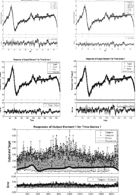
Figure 1 is the time series plot of OVX and crude oil price futures in terms of WTI and USO. The first panel exhibits an asymmetric correlation between WTI/USO and OVX prices. The price fluctuation is more evident around the period 2007–09. The year 2007–09 is the period of global financial crises during this period crude oil price crossed its highest limit and reached on its peak $160 and tumbled at the low level, below $20. Since crude lost its peak in 2009 and onwards and kept on ranging from $20 to $160, and still, it is struggling to find the best price globally. The time series variable shows a regime shift. Hence, Bai and Perron breakpoint least squares regression has been performed to analyze the prolonged relation between OVX and crude oil prices (e.g., Rafiq et al., 2009). The second panel clearly shows that OVX appears higher subject to crude measures of WTI and USO returns. It is seen OVX remains more volatile during 2007–09 and again jumped during 2015–16. Table 3 shows the diagnostic tests for the stationarity of time series variables. It is apparent that the null hypothesis “time series variable has unit root” is rejected for OVX, WTI, and USO in change.

Results and Discussion

observations for trading volume: it dips about 45,000 but maintains its range between 80,000-90,000, and sometimes it remains constant to this benchmark range. The lowest price does come over fairly later in the period. The concern is that the neural network yielded a bad outcome for the trading volume. The observed trading volume and predicted level appear to be larger with the highest amount of standard

deviation. Hence, the trading volume could not be taken as a good parameter for the forecasting of the future level of OVX market volatility. The volume parameter appears to be very skewed and cannot be used as input for the forecast of future price of crude oil.

Figure 1. Times Series Plot of OVX, WTI and USO

So now it has been found that what all parameters should be taken so as to predict the OVX, volumes parameter can be safely discarded. Figure 3 exhibits the level of the expected volatility of the crude oil market in terms of OVX. Figure 3 shows the OVX level by taking all parameters together into the neural network except for trading volume. Figure 3 is in line with the previous graph in which trajectories can be observed following the various prices of crude oil. It represents the reliability of the data and the forecast using the neural network model. Hence, one can say that ANN based forecast and observed OVX values are indistinguishable with minimal error. When looking at the error histogram, one can see that OVX prediction and test data form a normal distribution central to the zero-error mark. More specifically, it is seen that a maximum chunk of the data falls with the -3/+4 mark. Hence, it is evidenced that in the absence of trading volume, ANN based OVX forecast is the most optimal model1_.

On the asymmetric relation between crude oil price and oil market volatility assessed using the quantile regression model. The quantile regression outcome is more robust than the simple OLS estimates. Table 4 shows the median linear

1 _{Due to space constraints error histogram has not been placed here, it can} be available on request.

quantile regression results for various 𝜏 − 𝑞𝑢𝑎𝑛𝑡𝑖𝑙𝑒𝑠. Panel A reports the effects of WTI at 𝜏 − 0.10 appears to be -0.280 with t-stats -8.10; this indicates that crude oil price fluctuations impact on the OVX level negatively. It is seen across all other 𝜏 − 𝑞𝑢𝑎𝑛𝑡𝑖𝑙𝑒𝑠 on an average the slope of the WTI prices appears to be -0.34 and statistically significant. It also implies that OVX changes are subject to price fluctuation of WTI spot prices. The changes in the OVX remains on the higher side when WTI fluctuates more and options based on WTI futures causes a higher amount of premium for put options (e.g., Christoffersen & Pan 2017). This kind of market rally results in higher pressure on the put options which outcomes into higher premium and consequently high level of OVX. Panel B reports the estimates based on USO-ETF prices across all the 𝜏 −

𝑞𝑢𝑎𝑛𝑡𝑖𝑙𝑒𝑠 on an average coefficient of USO appears to be

Figure 3. Predicting OVX Level Based on WTI Prices

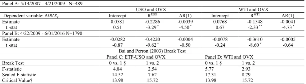
Graphical observation from Figure 1 exhibits that there is a shift in the time series. When the times series variable does have a break, it is essential to obtain the results based on the structural breaks. Bai and Perron (2003) test show that there is at least one break present in the time series under investigation. When applying Bai and Perron test on the values of OVX, WTI, and USO, it is found that there are two sub-periods. Period-1 consists of 05/2007 to 04/2009 with 489 observations; this is the global financial crisis period during which global crude price reached its all-time high level. Period-2 ranges from 04/2009 to 05/2016 with 1790 observations, during this period, crude oil prices tumble from its peak to lowest about $20 globally, and OVX level crossed the level of 100. Panel A of Table 5 shows that

the respective slopes of USO and WTI returns appears to be -0.23 and -0.15 and statistically significant.; this implies that OVX prices remain more volatile subject to oil price fluctuations during the crises period. One of the important observations from Panel B is that the slope of the USO and WTI are higher negative on the counterpart of the turbulence period. After the crisis period, the crude price falls dramatically from its peak level to the lowest level. The reason the OVX level has been rising significantly. Investors were buying more hedge funds to manage their oil price uncertainty. The excessive burden over put options and short position results in a higher level of implied volatility, and consequently, the OVX level jumped intensely.

Table 4

Quantile Regression Estimates

Panel A Regressor: WTI Prices (Median depend. var −10.00000 S.D. dependent var 225.2493)

Quantiles 0.10 0.20 0.30 0.40 0.50 0.60 0.70 0.80 0.90 Intercept -168.93 -103.38 -65.01 -35.75 -8.23 17.38 51.21 98.71 175.53 t-stat -27.27 * _-23.91 * _-20.88* _-12.09 * _-2.94 * _5.49 * _13.28 * _22.18 * _20.30 * RFWTI _{-0.28 -0.32 -0.33 -0.34 -0.34 -0.34 -0.35 -0.35 -0.38} t-stat -8.10 * _-13.20 * _-20.31 * _-20.49 * _-21.96 * _-94.67 * _-16.39 * _-14.45 * _-8.12 * Panel B Regressor: USO ETF prices (Median depend. var −10.00005 S.D. dependent var 225.3975)

Intercept -177.35 -106.96 -69.03 -36.81 -9.49 17.72 53.80 96.94 178.94 t-stat -27.02 * _-25.96 * _-20.69 * _-13.23 * _-3.49 * _5.65 * _14.12 * _21.38 * _19.34 * RFUSO _{-0.41 -0.48 -0.51 -0.48 -0.47 -0.52 -0.55 -0.58 -0.60} t-stat -6.66 * _-13.86 * _-15.01 * _-17.97 * _-17.23* _-19.37 * _-15.19 * _-13.11 * _-6.46 * [Table shows LQR estimation results. Standard errors are computed according to the asymptotic formula given by Koenker and Bassett (1978). Significant at *_{1 %, Robust (sandwich) standard errors]}

Table 5

Bi and Perron Break Least Squares

Panel A: 5/14/2007 - 4/21/2009 N=489

USO and OVX WTI and OVX

Dependent variable: ∆𝑂𝑉𝑋𝑡 Intercept RUSO _{AR(1) Intercept R}WTI _AR(1) Estimate 0.0581 -0.2286 -0.0039 0.0768 -0.1548 -0.0041

t -stat 0.51 -3.29 * _-4.50 * _{0.67 -2.33} ** _-4.73 *

Panel B: 4/22/2009 - 6/01/2016 N=1790

Estimate -0.0282 -0.4220 -0.0004 -0.0078 -0.3610 -0.0005

t -stat -0.87 -9.62 * _{-0.50 -0.24 -8.60} * _-0.64

Bai and Perron (2003) Break Test

Panel C: ETF-USO and OVX Panel D: WTI and OVX

Break Test 0 vs. 1 § 1 vs. 2 0 vs. 1 § 1 vs. 2

F-statistic 4.84 2.54 5.77 2.93

Scaled F-statistic 14.52 7.62 17.31 8.79

Critical Value† 13.98 15.72 13.98 15.72

Conclusion

The study aims to explain the crude oil price volatility based on the daily prices of OVX, WTI, and USO. The sample period covered in this study is 05/2007 to 05/2016. The present work is comprehensive; the reason it deals with forecasting crude oil prices using ANN and explaining the asymmetric relation between OVX and crude oil prices. The study employs ANN to find the most appropriate parameters which can be used to predict future prices and their relation with the volatility of the commodity. The OVX volatility index is taken during this study and available from CBOE daily, depending upon the options trading. The crude oil market volatility is articulated in terms of OVX throughout the study. The relationship of OVX concerning crude oil prices is completed with two bases. Firstly, with the neural networks and secondly quintile regression. Artificial Neural Network clearly explains that various historical prices of WTI/USO can be used to forecast the future prices of crude oil prices. Moreover, it is seen that volume does not add any values in forecasting since it is very noisy input. ANN estimates explain that future prices of WTI/USO can be predicted with minimal error. It can also be used to predict future crude oil market volatility.

The quantile regression results suggest that crude oil prices and OVX are strongly associated. The asymmetric association between WTI/USO and OVX explains that the volatility feedback effect holds good for the OVX market. Quantile regression speaks that WTI/USO and OVX are negatively associated. This supports the hypothesis of volatility feedback and leverage effects (e.g., Aboura & Chevallier 2013). Additionally, Bi and Perron breakpoint least squares presented in times series analysis and evidence the presence of a break in the time series. It is observed that the post crises period has caused significantly to the investors’ sentiment gauged in terms of OVX prices. The crude oil prices remain lower during this period; consequently, the OVX level appears to be higher. It also signifies that the market participant’s fear and anxiety about the future decrease in oil prices. The results uncover the fact that implied volatility (OVX) tends to remain calm during the global financial crises and higher throughout the post crises period. The empirical outcome on the OVX market provides some practical implications for the trader and investor: Oil futures can serve better in order to hedge the price volatility of crude oil. The crude oil producer can short hedge enough through volatility futures and options (F&O) to maintain the future quantity of crude to be produced.

References

Aboura, S., & Chevallier, J. (2013). Leverage vs. feedback: Which effect drives the oil market? FinanceResearch Letters, 10(3), 131–141. https://doi.org/10.1016/j.frl.2013.05.003.

Agnolucci, P. (2009). Volatility in crude oil futures: a comparison of the predictive ability of GARCH and implied volatility models. Energy Economics, 31(2), 316–321. https://doi.org/10.1016/j.eneco.2008.11.001

Ajmi, A. N., Gupta, R., Babalos, V., & Hefe, R. (2015). Oil price and consumer price nexus in South Africa revisited: A novel asymmetric causality approach. Energy Exploration & Exploitation, 33(1), 63–73. https://doi.org/10.1260%2F0 144-5987.33.1.63.

Al‐Abri, A. S. (2013). Oil price shocks and macroeconomic responses: does the exchange rate regime matter? OPEC Energy Review, 37(1), 1–19. https://doi.org/10.1111/j.1753-0237.2012.00226.x.

Alexander, C. (2008). Market risk analysis: Practical financial econometrics (Vol. II). England: Hoboken: Wiley.

Amano, R. A., & Norden, S. V. (1998). Oil prices and the rise and fall of the US real exchange rate. Journal of international Money and finance, 17(2), 299–316. https://doi.org/10.1016/S0261-5606(98)00004-7.

Arouri, M. E., Lahiani, A., & Nguyen, D. K. (2011). Return and volatility transmission between world oil prices and stock markets of the GCC countries. Economic Modelling, 28(4), 1815–1825. https://doi.org/10.1016/j.econmod. 2011.03.012.

Awartani, B., Aktham, M., & Cherif, G. (2016). The connectedness between crude oil and financial markets: Evidence from implied volatility indices. Journal of Commodity Markets, 4(1), 56–69. https://doi.org/10.1016/j.jcomm. 2016.11.002.

Bai, J., & Perron, P. (2003). Computation and analysis of multiple structural change models. Journal of applied econometrics, 18(1), 1–22. https://doi.org/10.1002/jae.659. https://doi.org/10.1002/jae.659

Bashiri, N., Bastianin, A., Bortolussi, E., Conti, F., Manera, M., & Nicolini, M. (2015). Current Issues on the Price of Oil: Decline, Forecasting, Volatility and Uncertainty. Review of Environment, Energy andEconomics, July 9, 2015, 1–8. Bates, D. S. (2000). Post-'87 crash fears in the S&P 500 futures option market. Journal of Econometrics, 94(1-2), 181–238.

https://doi.org/10.1016/S0304-4076(99)00021-4.

Bein, M. A. (2017). Time-Varying Co-Movement and Volatility Transmission between the Oil Price and Stock Markets in the Baltics and Four European Countries. Inzinerine Ekonomika-Engineering Economics, 28(5), 482–493. http://dx.doi.org/10.5755/j01.ee.28.5.17743.

Bollerslev, T., & Zhou, H. (2006). Volatility puzzles: a simple framework for gauging return-volatility regressions. Journal of Econometrics, 131(1/2), 123–150. https://doi.org/10.1016/j.jeconom.2005.01.006

Campbell, J., & Hentschel, L. (1992). No News is Good News: An Asymmetric Model of Changing Volatility in Stock Returns. Journal of Financial Economics, 31(3), 281–318. https://doi.org/10.1016/0304-405X(92)90037-X.

CBOE. (2008). CBOE INTRODUCES NEW CRUDE OIL VOLATILITY INDEX (OVX); New Benchmark Applies VIX Methodology To Options On The United States Oil Fund (USO). Chicago: Cboe Options Exchange (Cboe).

Chen, Y., & Zou, Y. (2015). Examination on the relationship between OVX and crude oil price with Kalman filter. Procedia Computer Science, 55, 1359–1365. https://doi.org/10.1016/j.procs.2015.07.122.

Christie, A. A. (1982). The stochastic behavior of common stock variances:value, leverage and interest rate effects. Journal of Financial Economics, 10(4), 407–432. https://doi.org/10.1016/0304-405X(82)90018-6.

Christoffersen, P., & Pan, X. N. (2017). Oil volatility risk and expected stock returns. Journal of Banking& Finance, 95, 5–26. https://doi.org/10.1016/j.jbankfin.2017.07.004.

Conrad, C., Loch, K., & Rittler, D. (2014). On the macroeconomic determinants of long-term volatilities and correlations in US stock and crude oil markets. Journal of Empirical Finance, 29, 26–40. https://doi.org/10.1016/j.jempfin. 2014.03.009.

Dennis, P., Mayhew, S., & Stivers, C. (2006). Stock Returns, Implied Volatility Innovations, and the Asymmetric Volatility Phenomenon. Journal of Financial and Quantitative Analysis, 41(2), 381–406. https://doi.org/10.1017/S002210900 0002118.

Dowling, S., & Muthuswamy, J. (2005). The implied volatility of Australian index options. Review ofFutures Markets, 14(1), 117–155. https://dx.doi.org/10.2139/ssrn.500165.

Dutta, A. (2017). Oil price uncertainty and clean energy stock returns: New evidence from crude oil volatility index. Journal of Cleaner Production, 164, 1157–1166. https://doi.org/10.1016/j.jclepro.2017.07.050.

Ederington, L. H., & Guan, W. (2010). How asymmetric is U.S. stock market volatility? Journal ofFinancial Markets, 13(2), 225–248. https://doi.org/10.1016/j.finmar.2009.10.001.

EIA. (2019, November 27). What Drives Crude Oil Prices? Retrieved from Energy & Financial Markets, U.S. Energy Information Administration: https://www.eia.gov/finance/markets/crudeoil/spot_prices.php

Fleming, J., Ostdiek, B., & Whaley, R. E. (1995). Predicting stock market volatility: A new measure. Journal of Futures Markets, 15(3), 265–302. https://doi.org/10.1002/fut.3990150303.

Fong, W. M., & See, K. H. (2002). A Markov switching model of the conditional volatility of crude oil futures prices. Energy Economics, 24(1), 71–95. https://doi.org/10.1016/S0140-9883(01)00087-1.

French, K. R., Schwert, G. W., & Stambaugh, R. F. (1987). Expected stock returns and volatility. Journalof Financial Economics, 19(1), 3–29. https://doi.org/10.1016/0304-405X(87)90026-2.

Frijns, B., Tallau, C., & Tourani-Rad, A. (2010a). The information content of implied volatility: Evidence from Australia. Journal of Futures Markets, 30(2), 134–155. https://doi.org/10.1002/fut.20405.

Frijns, B., Tallau, C., & Tourani-Rad, A. (2010b). Australian Implied Volatility Index. Jassa the finsiajournal of applied finance, 10 (1), 31–35.

Galyfianakis, G., Garefalakis, A., & Mantalis., G. (2017). The Effects of Commodities and Financial Markets on Crude Oil. Oil & Gas Science and Technology-Revue d'IFP Energies nouvelles, 72(1), 3. https://doi.org/10. 2516/ogst/2016024.

Ghassan, H. B., & AlHajhoj, H. R. (2016). Long run dynamic volatilities between OPEC and non-OPEC crude oil prices. Applied Energy, 169, 384–394. https://doi.org/10.1016/j.apenergy.2016.02.057.

Giot, P. (2005). Relationships between implied volatility indices and stock index returns. Journal of Portfolio Management, 31(3), 92–100. https://doi.org/10.3905/jpm.2005.500363.

Haugom, E., Langeland, H., Molnar, P., & Westgaar, S. (2014). Forecasting volatility of the US oil market. Journal of Banking & Finance, 47, 1–14. https://doi.org/10.1016/j.jbankfin.2014.05.026.

Jouini, J. (2013). Return and volatility interaction between oil prices and stock markets in Saudi Arabia. Journal of Policy Modeling, 35(6), 1124–1144. https://doi.org/10.1016/j.jpolmod.2013.08.003.

Koenker, R., & Bassett, J. G. (1978). Regression quantiles. Econometrica: journal of the EconometricSociety,, 33–50. https://www.jstor.org/stable/1913643. https://doi.org/10.2307/1913643

Latane, H. A., & Rendleman, R. J. (1976). Standard Deviations of Stock Price Ratios Implied in Option Prices. The Journal of Finance, 31( 2), 369-38. https://doi.org/10.1111/j.1540-6261.1976.tb01892.x.

Liu, M. L., Ji, Q., & Fan, Y. (2013). How does oil market uncertainty interact with other markets? An empirical analysis of implied volatility index. Energy, 55, 860–868. https://doi.org/10.1016/j.energy.2013.04.037.

Low, C. (2004). The fear and exuberance from implied volatility of S&P 100 index options. The Journal of Business,, 77(3), 527–546. https://www.jstor.org/stable/10.1086/386529.

Luo, X., & Qin, S. (2017). Oil price uncertainty and Chinese stock returns: New evidence from the oil volatility index. Finance Research Letters, 20, 29–34. https://doi.org/10.1016/j.frl.2016.08.005.

Maghyereh, A. I., Awartani, B., & Bouri., E. (2016). The directional volatility connectedness between crude oil and equity markets: New evidence from implied volatility indexes. Energy Economics, 57, 78–93. https://doi.org/10.10 16/j.eneco.2016.04.010.

Martens, M., & Zein, J. (2004). Predicting financial volatility: High‐frequency time‐series forecasts vis‐à‐vis implied volatility. Journal of Futures Markets, 24(11), 1005–1028. https://doi.org/10.1002/fut.20126.

Masih, R., Peters, S., & Mello, L. D. (2011). Oil price volatility and stock price fluctuations in an emerging market: evidence from South Korea. Energy Economics, 33(5), 975–986. https://doi.org/10.1016/j.eneco.2011.03.015.

Nakanishi, T., & Komiyama, R. (2006). Supply and Demand Analysis on Petroleum Products and Crude Oils for Asia and the World. The Institute of Energy Economy, Tokyo, Japan: IEEJ.

Narayan, P. K., & Narayan, S. (2007). Modelling oil price volatility. Energy policy, 35(12), 6549–6553. https://doi.org/10. 1016/j.enpol.2007.07.020.

Poteshman, A. M. (2001). Underreaction, Overreaction, and Increasing Misreaction to Information in the Options Market. The Journal of Finance, 56(3), 851–876. https://doi.org/10.1111/0022-1082.00348.

Rafiq, S., Salim, R., & Bloch, H. (2009). Impact of crude oil price volatility on economic activities: An empirical investigation in the Thai economy. Resources Policy, 4(3), 121–132. https://doi.org/10.1016/j.resourpol.2008.09.001. Schwert, G. W. (1989). Why does stock market volatility change over time? The Journal of Finance, 44(5), 1115–1153.

https://doi.org/10.1111/j.1540-6261.1989.tb02647.x.

Schwert, G. W. (1990). Stock Volatility and the Crash of '87. Review of Financial Studies, 3(1), 77–102. https://doi.org/10. 1093/rfs/3.1.77.

Shaikh, I. (2018). Investors' fear and stock returns: Evidence from National Stock Exchange of India. Inzinerine Ekonomika-Engineering Economics, 29(1), 4–12. http://dx.doi.org/10.5755/j01.ee.29.1.14966.

Soltes, V., & Harcarikova, M. (2017). Design of New Barrier Outperformance Certificates in Oil Market. Inzinerine Ekonomika-Engineering Economics, 28(3), 262–270. http://dx.doi.org/10.5755/j01.ee.28.3.11481.

Warin, T., & Sanger, W. (2018). Connectivity and closeness among international financial institutions: a network theory perspective. International Journal of Comparative Management, 1(3), 225–254. https://dx.doi.org/10.1504/IJCM. 2018.094479.

Wei, Y., Wang, Y., & Huang, D. (2010). Forecasting crude oil market volatility: Further evidence using GARCH-class models. Energy Economics, 32(6), 1477–1484. https://doi.org/10.1016/j.eneco.2010.07.009.

Whaley, R. E. (2000). The Investor Fear Gauge. The Journal of Portfolio Management, 26(3), 12–17. https://doi.org/10. 3905/jpm.2000.319728.

Zhu, F., Zhu, Y., Jin, X., & Luo, X. (2017). Do spillover effects between crude oil and natural gas markets disappear? Evidence from option markets. Finance Research Letters, 24, 25–33. https://doi.org/10.1016/j.frl.2017.05.007.