Science Data

(1)

Earth Syst. Sci. Data, 6, 147–164, 2014 www.earth-syst-sci-data.net/6/147/2014/ doi:10.5194/essd-6-147-2014

©Author(s) 2014. CC Attribution 3.0 License. _Open

Access

Earth System

Science

Data

High-resolution atmospheric reconstruction for Europe

1948–2012: coastDat2

B. Geyer

Institute of Coastal Research, Helmholtz-Zentrum Geesthacht, Geesthacht, Germany

Correspondence to: B. Geyer ([email protected])

Received: 5 November 2013 – Published in Earth Syst. Sci. Data Discuss.: 2 December 2013 Revised: 20 March 2014 – Accepted: 25 March 2014 – Published: 17 April 2014

Abstract. The coastDat data sets were produced to give a consistent and homogeneous database mainly for assessing weather statistics and climate changes since 1948, e.g., in frequencies of extremes for Europe, es-pecially in data sparse regions. A sequence of numerical models was employed to reconstruct all aspects of marine climate (such as storms, waves, surges, etc.) over many decades. The acronym coastDat stands for the set of consistent ocean and atmospheric data, where the atmospheric data where used as forcing for the reconstruction of the sea state. Here, we describe the atmospheric part of coastDat2 (Geyer and Rockel, 2013; doi:10.1594/WDCC/coastDat-2_COSMO-CLM). It consists of a regional climate reconstruction for the entire European continent, including the Baltic Sea and North Sea and parts of the Atlantic. The simulation was done for 1948 to 2012 with the regional climate model COSMO-CLM (CCLM) and a horizontal grid size of 0.22 degree in rotated coordinates. Global reanalysis data of NCEP1 were used as forcing and spectral nudging was applied. To meet the demands on the coastDat data set about 70 variables are stored hourly.

1 Motivation

The precursor of coastDat2, coastDat1 (Weisse et al., 2009), was widely used. About 50 % of the coastDat1 users were commercial, while 25 % were academic and another 25 % were from the authorities. Applications range from assess-ing long-term variability and change to risk assessment and design, for example of offshore wind farms. As coastDat1 terminated in 2007, and as there were strong requests for an upgrade comprising the most recent years at higher spa-tial resolution, the coastDat2 effort was implemented. The atmospheric part of coastDat2 described in this paper was produced with the community model COSMO-CLM on the current super computer of the German Climate Computing Center (DKRZ). It is the successor of the coastDat1 regional atmospheric simulation done with REMO5.0 (Feser et al., 2001; Jacob et al., 2001). For coastal areas the higher res-olution is the main advantage. The overall advantage is the availability of the last 5 years.

2 Model setup

For the reconstruction the COSMO model in CLimate Mode (COSMO-CLM) version 4.8_clm_11 (Rockel et al., 2008; Baldauf et al., 2011; Steppeler et al., 2003) was used. The COSMO model is the non-hydrostatic opera-tional weather prediction model applied and further devel-oped by the national weather services affiliated in the COn-sortium for SMall-scale MOdeling (COSMO). The climate mode is applied and developed by the Climate Limited-area Modelling Community (http://www.clm-community. eu). The use of the model is well supported by the members of the community and documented mainly via the COSMO documentation (http://www.cosmo-model.org/ content/model/documentation/core/default.htm).

The simulation was done on a regular grid in rotated co-ordinates with a rotated pole at 170.0◦_{W and 35.0}◦_{N with}

a resolution of 0.22◦_{, a time step of 150 s and hourly}

(2)

Figure 1.Orography [m] of model domain of cpastDat2-CCLM (colored area). The white frame indicates the 10 pixel wide sponge zone. The red boxes define the borders of the eight European stan-dard evaluation domains defined by Rockel and Woth (2007).

upper levels (above 850 hPa) to enforce the observed large-scale circulation. Every fifth time step, in both directions, the information of the five largest wavelengths was nudged with a nudging factor of 0.5. A detailed description of the tech-nique was provided by Müller (2003, p. 50). At the lateral boundaries the relaxation scheme by Davies (1976) was ap-plied. The affected 10 grid boxes, the sponge zone, are cut offfor all time series data of the set.

Meteorological initial and boundary conditions were taken from the 6 hourly NCEP1 reanalysis data (Kalnay et al., 1996; Kistler et al., 2001). The simulation was initialized on first of January 1948 with interpolated fields for the air tem-perature, zonal and meridional wind component, specific wa-ter vapor content, specific cloud wawa-ter content, surface spe-cific humidity, skin temperature for sea points, thickness of surface snow amount and volume fraction of soil moisture. The interpolation to the coastDat2-CCLM grid was done by the model chain part int2lm v1.9_clm5 (Schättler, 2011). The soil moisture values of the coarse NCEP grid require more spin up time than the few days required by atmospheric fields (Denis et al., 2002). Therefore it is necessary to run the model for a certain time and to restart with the gained soil moisture fields. Figure 2 shows the development of the moisture for area means of layers 1–8 for the European standard evalua-tion areas (Rockel and Woth, 2007) adopted by Christensen and Christensen (2007, p. 22). The layers 9–10 are hydro-logically not active, the water draining through layer 8 was

Figure 2.Soil moisture content [m] for the eight European sub-regions of Fig. 1. Crosses: initial value; dashed lines: monthly mean of spin up run; solid: monthly mean of the final (restarted) simula-tion. The colors belong to the soil levels.

added to the runoff. Layer 7 and 8 have the same start value of 0.33 m. The end of the spin up period is where both soil mois-ture fields (soil moismois-ture content of spin up simulation and soil moisture content of coastDat2-CCLM) converge. The re-quired time depends on the accuracyof the initial condition and therefore differs between the regions. The largest spin up time of 5 years can be found for eastern Europe. There-fore we choose 1948–1952 as spin up time and restarted the coastDat2-CCLM simulation on the first of January 1948 as before with the same initial conditions except for soil mois-ture, where we used the gained values from the spin up sim-ulation.

Land surface processes were parameterized with the TERRA-ML scheme (Schrodin and Heise, 2001; Doms et al., 2011). For sea points the NCEP1 skin temperatures were used as lower boundary condition. Cumulus convection was parameterized using the Tiedtke scheme (Tiedtke, 1989). Clouds were determined by the prognostic variables cloud water and cloud ice. We used a fifth order Runge–Kutta time integration scheme.

The hourly output was written in netCDF following the CF-conventions 1.4 (Eaton et al., 2009). In the appendix (Ta-ble A1) all output varia(Ta-bles are listed.

3 External data

(3)

B. Geyer: High-resolution atmospheric reconstruction: coastDat2 149

Figure 3.Mean differences of monthly mean 2 m air temperatures [K] from 1950 to 2012: coastDat2-CCLM minus E-OBS8.0.

soil temperature was taken from the CRU (Climate research Unit at the University of East Anglia). To generate a file with the merged information on the model grid, the so-called PrE-Processor (PEP) was used. Detailed information on the data as well as the preprocessor is given by Smiatek et al. (2008). The list of used climatological input variables are included in Table A1.

4 Evaluation

The evaluation was done for several parameters. The user de-mands are manifold, ranging from coastDat-internal forcing for the wave model via air chemistry models to research in the field of wind energy. In this paper we show data set com-parisons for the most user-requested quantities: 2 m tempera-ture, total precipitation, wind speed, cloud cover, and height of boundary layer.

4.1 Reference data sets

The evaluation of the data set for air temperature, precipi-tation, wind, and cloud cover was done by using common gridded data sets: E-OBS of the ENSEMBLES project ver-sion 8.0 (van den Besselaar et al., 2011; Haylock et al., 2008), CRU version ts_3.2 (Jones and Harris, 2011), GPCC

(Global Precipitation Climatology Centre), version 6 (Rudolf et al., 2010), and REGNIE from Deutscher Wetterdienst (Di-etzer, 2000). For comparison of the height of boundary layer we used station data for Lindenberg, Germany (Beyrich and Leps, 2012).

4.2 Near-surface air temperature

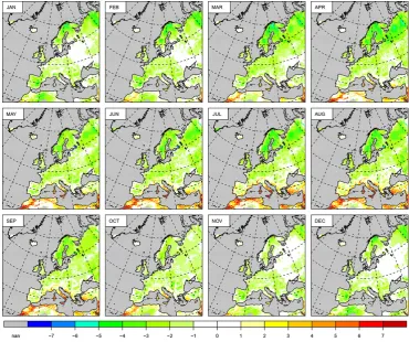
Figure 3 shows the mean differences between the monthly means of air temperature at 2 m height of coastDat2-CCLM and E-OBS8.0 for 1950–2012. The E-OBS data were inter-polated to the rotated grid of CCLM.

From April to September, the differences are between

−1◦C and 1◦C for wide areas of mid-Europe. High diff er-ences with values up to −6 and +6◦_{C occur over Iceland}

(4)

Figure 4.Correlations between coastDat2-CCLM and E-OBS8.0 of monthly mean 2 m air temperatures from 1950 to 2012.

(5)

Figure 6.Differences of mean monthly sums of total precipitation [mm] from 1950 to 2012: coastDat2-CCLM minus E-OBS8.0.

For Africa Kothe et al. (2014) found that the used albedo values are to low compared to satellite data (Kothe et al., 2014, Fig. 2), which leads to higher temperatures in summer. At the time when the coastDat2-CCLM simulation was started the new albedo data set was not yet available. The statistical significance on the 0.05 % level of the 2 m tem-perature differences was tested separately for 12 month to avoid auto correlation. It yields for large regions statistically significant values between observation and CCLM simula-tion. This result is, however, not surprising because of in-herent model biases of the forcing NCEP1 data. To give an additional hint on the quality of the time series in Fig. 4, the correlations between CCLM and E-OBS8.0 are shown. Here the correlations are over large areas statistically significant and coastDat2-CCLM represents a large part of the observed variance.

The precursor data set, coastDat1, was used as forcing for biosphere models (e.g., (Jung et al., 2007) or (Vetter et al., 2008)), where the diurnal cycle has major impor-tance. Therefore, we determined the differences of the di-urnal temperature range. It was calculated as the difference

between daily maximum 2 m air temperature and daily min-imum 2 m air temperature. The means of the monthly mean differences between coastDat2-CCLM and E-OBS8.0 for the period 1950–2012 are shown in Fig. 5.

There is a tendency to underestimate the diurnal temper-ature range for wide areas all over the year, except for the part of North Africa contained in the model domain. The differences in the maximum 2 m air temperature are highest for April–August. In the North African part the coastDat2-CCLM temperatures are several degrees higher than the val-ues of E-OBS and in the northeastern parts of Europe they are several degrees lower than the observations (not shown). The differences between the two data sets in minimum 2 m air temperature are much smaller, with the highest deviations occurring for Africa from June to August (not shown). The main source for the differences in the diurnal temperature range is the difference in maximum 2 m air temperature.

4.3 Precipitation

(6)

Table 1.Seasonal-mean minimal differences of precipitation [%] over land between coastDat2-CCLM and the ensemble of the three obser-vational data (E-OBS, CRU, GPCC) for 1950–2010 and the eight European sub-regions of Fig. 1: British Islands (A1), Iberian Peninsula (A2), France (A3), mid-Europe (A4), Scandinavia (A5), Alps (A6), Mediterranean (A7), eastern Europe (A8). Values less than 10 % are printed bold.

A1 A2 A3 A4 A5 A6 A7 A8

DJF −1.2 3.9 6.4 15 20 7.8 −0.3 24

MAM 2.1 0.2 1.1 7.7 43 9.5 −1.8 11

JJA −9.6 −34 −29 −23 2.1 −17 −42 −33 SON −9.4 −17 −14 −6.7 7.0 −14 −23 −16

Figure 7.Differences of mean monthly sums of total precipitation [mm] from 1950 to 2010: coastDat2-CCLM minus GPCC6.

E-OBS8.0. The basis is the period 1950–2012, the E-OBS data are interpolated to the rotated grid of CCLM. Main de-viations occur on the one hand in spring over Scandinavia and the northeastern part of the model domain, with more simulated precipitation than E-OBS reconstructed. On the other hand, we have less precipitation in southeastern Europe in summer. The tendency to precipitation values higher than E-OBS8.0 in Northern Europe is stronger and occurs over the entire year in the precursor atmospheric simulation with REMO-SN (belonging to coastDat1) as well as the lower

val-ues in July to September in southern part of mid-Europe (not shown).

(7)

Figure 8a.Area mean monthly sums of total precipitation of December, January, and February of 1950–2010: coastDat2-CCLM (red), range of GPCC6, E-OBS8.0 and CRU3.2 for each season (gray filled).

GPCC6 shows 5–10 mm higher monthly summer precipita-tion in eastern Europe (not shown). Strong deviaprecipita-tions be-tween GPCC6 and E-OBS8.0 occur for Iceland from Octo-ber to April and Turkey from DecemOcto-ber to February, with up to 100 mm month−1 _{and up to 60 mm month}−1_,

(8)

Figure 8b.Area mean monthly sums of total precipitation of March, April, and May of 1950–2010: coastDat2-CCLM (red), range of GPCC6, E-OBS8.0 and CRU3.2 for each season (gray filled).

To use the information on the spread of the data sets based on observations (E-OBS, GPCC and CRU), we calculated the mean minimal differences between coastDat2-CCLM and the three observational data sets and listed them as percentages in Table 1.

(9)

Figure 8c.Area mean monthly sums of total precipitation of June, July, and August of 1950–2010: coastDat2-CCLM (red), range of GPCC6, E-OBS8.0 and CRU3.2 for each season (gray filled).

from June to August for the Iberian Peninsula (A2), June to November for Mediterranean (A7) and June to August in eastern Europe (A8), while systematic highest positive deviations are found from December to May in Scandinavia (A5). In addition to the table, we show the monthly mean

(10)

Figure 8d.Area mean monthly sums of total precipitation of September, October, and November of 1950–2010: coastDat2-CCLM (red), range of GPCC6, E-OBS8.0 and CRU3.2 for each season (gray filled).

some users of our data set are interested in especially dry or wet seasons, we show absolute values. It becomes clear, that the deviations between the observational data sets are huge (e.g., for Mediterranean from June to November or the Alps

in summer). But nevertheless the model mean is outside the gridded observational data set range in various cases.

(11)

Figure 9.Histogram of Germany mean daily precipitation sums [mm] from 1951 to 2009: REGNIE (red bars), coastDat2-CCLM (blue bars), and E-OBS8.0 (shaded).The frequency is given in %.

Figure 10. Validation of near-surface wind speeds: quantile– quantile plot for Atlantic offshore conditions (left: 2007–2012, plat-form K1 height corrected) and near-shore Mediterranean conditions (right: 2000–2012, buoy Athos).

possibility of statistics on a daily basis. Figure 9 shows a his-togram of area mean daily precipitation for Germany. The borders of the classes were chosen following the recommen-dation of the Global Precipitation Climatology Project.

The shape of the REGNIE distribution function is gener-ally well reproduced in coastDat2-CCLM. However, only for the two classes from 1.7 to 3 mm day−1 _{for all seasons the} three data sets (REGNIE, coastDat2-CCLM and E-OBS8.0) show the same frequencies. For all other classes no consis-tent statement concerning relation between the data sets is possible.

4.4 Wind

The modified Brier skill score was calculated following Win-terfeldt et al. (2010). They found an added value of the regional atmospheric simulation of coastDat1, done with REMO5.0, compared to the forcing reanalysis of NCEP with satellite data of quikScat near the coasts. These findings were reproduced for the coastDat2-CCLM data set. Important for users of our wind data is the proofed good offshore quality of the surface wind data, although the Brier skill score for wide offshore fields is negative, meaning that NCEP1 data has a higher agreement with observations than coastDat2-CCLM. As shown for the precursor data set, coastDat1, by Sotillo et al. (2005, Fig. 7), the quality (e.g., at platform K1) is very good. Following the idea of Sotillo et al., our Fig. 10 shows the quantile–quantile plot of observation vs. model data (blue coastDat2-CCLM and red NCEP1). On the left hand side, results are for Atlantic buoy K1 (at 48.701◦N, 12.401◦_{W) and on the right hand side for Aegean Buoy}

Athos (at 39.97◦_{N, 24.72}◦_{E). K1 observations were}

(12)

Figure 11.Differences of mean monthly means of total cloud cover [1] from 1950 to 2010: coastDat2-CCLM minus CRU3.2.

4.5 Total Cloud Cover

The comparison of the total cloud cover of coastDat2-CCLM and CRU data is shown in Fig. 11. For most of the months and most of the areas the differences are below 10 %. The highest differences occur from June to August over North Africa and March to August over Scandinavia. For most of the year, the differences for Greenland are high.

4.6 Height of planetary boundary layer

Observational data for the height of the boundary layer are hardly available. As this variable is especially important when the coastDat data set is used for air chemistry ap-plications (i.e., to simulate the transport of harmful sub-stances), we show at least a comparison for a short-term period (2003–2012) at a single station (Lindenberg, WMO no. 10393, 52.21◦_{N, 14.10}◦_{E). As the height of the boundary}

layer shows a strong diurnal cycle, the data set was divided into four sets depending on the start time of the soundings. The start time of the soundings is 45 to 75 min prior to the re-porting time at 00:00, 06:00, 12:00, and 18:00 UTC.

There-fore the corresponding values from 23:00, 05:00, 11:00, and 17:00 UTC of the simulated data were selected. The observa-tions are flagged with quality status flags, which were derived by the use of four different methods to calculate the height of the PBL (Beyrich and Leps, 2012). From both data sets the values with observation quality flag “good” were extracted. For comparison both values were related to ground height, because real elevation is 112 m while the model height is 63 m.

Figure 12 shows the frequency distribution of boundary layer heights from model and observation by launch time and season. The classes refer to the model levels.

(13)

Figure 12.Frequency distribution of the planetary boundary layer height [m] of coastDat2-CCLM and observation from 2003 to 2012.

Table 2.Statistical parameters of the comparison between observed and simulated PBL height, split for sounding times in column 3 to 6, and seasons in rows according to the abbreviation in column 2. Listed are the number and the median of used observed values (me-dian O), me(me-dian of simulated values (me(me-dian S), and the differences of the medians. Unit of the last three variables is m.

00:00 06:00 12:00 18:00

number

DJF 490 647 678 598

MAM 486 630 665 633

JJA 574 700 690 641

SON 424 396 505 509

median O

DJF 220 136 98 127

MAM 202 136 125 124

JJA 384 1166 1310 661

SON 232 829 917 109

median S

DJF 356 258 258 258

MAM 356 258 258 258

JJA 475 1409 1669 964

SON 356 778 1174 258

difference

DJF 136 122 160 131

MAM 154 122 133 134

JJA 91 243 359 303

SON 124 −51 257 149

model levels (in the height of 213 m) are clearly lower than the observations.

In Table 2 the numbers of good-flagged deduced heights of PBL are listed per season and sounding time, the according medians of these and the CCLM simulated heights, as well as the differences of these values are shown.

All midnight to noon simulated median values are higher than those observed within a range of 90–260 m. Only the autumn 06:00 UTC simulated value is less than the one observed. Particular high are the differences for June to Au-gust 12:00 and 18:00 UTC soundings with more then 300 m.

5 Conclusions

(14)

The data of the atmospheric part of coastDat2, coastDat2-CCLM, (Geyer and Rockel, 2013) are downloadable from doi:10.1594/WDCC/coastDat-2_COSMO-CLM.

Acknowledgements. The CCLM is the community model of the German climate research (www.clm-community.eu). The German Climate Computing Center (DKRZ) provided the computer hardware for the Limited Area Modelling simulations in the project “Regional Atmospheric Modelling”. The NCEP/NCAR1 reanalysis data was provided by the National Center for Atmo-spheric Research (NCAR). Thanks to the ENSEMBLES group for updating the E-OBS data set according to newest findings, to the CRU crew providing the CRU time series, GPCC and DWD for allowing us to use their data. We thank the UK Met office for providing the wind measurements at Buoy K1 station number 62029. The Athos buoy data are available via the POSEIDON Operational Oceanography System, Hellenic Centre for Marine Research (http://www.poseidon.hcmr.gr). We thank Frank Beyrich for providing height of boundary layer data from Deutscher Wetterdienst for Lindenberg. Additionally we want to thank the providers of the external data sets (cited in detail by Smiatek et al., 2008): the FAO for soil-types data, and USGS for the orography, and Global ecosystem data. Last but not least we want to thank the both reviewers which helped with their comments and suggestions to improve the manuscript.

The service charges for this open access publication have been covered by a Research Centre of the Helmholtz Association.

Edited by: G. König-Langlo

References

Baldauf, M., Seifert, A., Förstner, J., Majewski, D., Raschendor-fer, M., and Reinhardt, T.: Operational Convective-Scale Nu-merical Weather Prediction with the COSMO Model: Descrip-tion and Sensitivities, Mon. Weather Rev., 139, 3887–3905, doi:10.1175/MWR-D-10-05013.1, 2011.

Beyrich, F. and Leps, J.: An operational mixing height data set from routine radiosoundings at Lindenberg: Methodology, Meteorol. Z., 21, 337–348, doi:10.1127/0941-2948/2012/0333, 2012. Bromwich, D. H., Bai, L., and Bjarnason, G. G.: High-Resolution

Regional Climate Simulations over Iceland Using Polar MM5*, Mon. Weather Rev., 133, 3527–3547, doi:10.1175/MWR3049.1, 2005.

Christensen, J. and Christensen, O.: A summary of the PRUDENCE model projections of changes in European climate by the end of this century, Clim. Change, 81, 7–30, doi:10.1007/ s10584-006-9210-7, 2007.

Davies, H. C.: A lateral boundary formulation for multi-level prediction models, Q. J. Roy. Meteor. Soc., 102, 405–418, doi:10.1002/qj.49710243210, 1976.

Denis, B., Laprise, R., Caya, D., and Cote, J.: Downscaling abil-ity of one-way nested regional climate models: the Big-Brother Experiment, Clim. Dynam., 18, 627–646, doi:10.1007/ s00382-001-0201-0, 2002.

Dietzer, B.: Berechnung von Gebietsniederschlagshöhen nach dem Verfahren REGNIE., Deutscher Wetterdienst – Hydrometeorolo-gie, Offenbach, 2000.

Doms, G., J., F., Heise, E., Herzog, H.-J., Mrionow, D., Raschendorfer, M., Reinhart, T., Ritter, B., Schrodin, R., Schulz, J.-P., and Vogel, G.: A Description of the Non-hydrostatic Regional COSMO Model. Part II: Physical Pa-rameterization, Tech. Rep., Deutscher Wetterdienst, available at: http://www.cosmo-model.org/content/model/documentation/ core/cosmoPhysParamtr.pdf (last access: 20 March 2014), 2011. Eaton, B., Gregory, Jonathan andDrach, B., Taylor, K., and Hankin, S.: NetCDF Climate and Forecast (CF) Metadata Conventions, Version 1.4, available at: https://github.com/cf-convention/cf-documents/blob/master/ cf-conventions/1.4/cf-conventions.pdf?raw=true (last access: 20 March 2014), 2009.

Einarsson, M. A.: Climate of Iceland, in: World survey of clima-tology, Climates of the Oceans, Chap. 7, 15 pp. 673–697, Else, Amsterdam, 1984.

Feser, F., Weisse, R., and von Storch, H.: Multi-decadal Atmo-spheric Modeling for Europe Yields Multi-purpose Data, EOS Transactions, 82, 305–310, doi:10.1029/01EO00176, 2001. Geyer, B. and Rockel, B.: coastDat-2 COSMO-CLM., World Data

Center for Climate. CERA-DB “coastDat-2_COSMO-CLM”, available at: http://cera-www.dkrz.de/WDCC/ui/Compact.jsp? acronym=coastDat-2_COSMO-CLM (last access: 20 March 2014), 2013.

Haylock, M. R., Hofstra, N., Tank, A. M. G. K., Klok, E. J., Jones, P. D., and New, M.: A European daily high-resolution gridded data set of surface temperature and precipitation for 1950–2006, J. Geophys. Res., 113, D20119, doi:10.1029/2008JD010201, 2008.

Jacob, D., Hurk, B. J. J. V. D., Andræ, U., Elgered, G., Fortelius, C., Graham, L. P., Jackson, S. D., Karstens, U., Köpken, C., Lindau, R., Podzun, R., Rockel, B., Rubel, F., Sass, B. H., Smith, R. N. B., and Yang, X.: A comprehensive model inter-comparison study investigating the water budget during the BALTEX-PIDCAP period, Meteorol. Atmos. Phys., 77, 19–44, 2001.

Jones, P. and Harris, I.: CRU Time Series (TS) high resolution grid-ded data version 3.10, NCAS British Atmospheric Data Centre, 2011.

Jung, M., Vetter, M., Herold, M., Churkina, G., Reichstein, M., Za-ehle, S., Cias, P., Viovy, N., Bondeau, A., Chen, Y., Trusilova, K., Feser, F., and Heimann, M.: Uncertainties of modeling gross pri-mary productivity over Europe: A systematic study on the effects of using different drivers and terrestrial biosphere models, Global Biogeochem. Cy., 21, GB4021, doi:10.1029/2006GB002915, 2007.

(15)

Kistler, R., Kalnay, E., Collins, W., Saha, S., White, G., Woollen, J., Chelliah, M., Ebisuzaki, W., Kanamitsu, M., Kousky, V., van den Dool, H., Jenne, R., and Fiorino, M.: The NCEP-NCAR 50-year reanalysis: Monthly means CD-ROM and documentation, B. Am. Meteorol. Soc., 82, 247–267, 2001.

Kothe, S., Lüthi, D., and Ahrens, B.: Analysis of the West African Monsoon system in the regional climate model COSMO-CLM, Int. J. Climatol., 34, 481–493, doi:10.1002/joc.3702, 2014. Müller, B.: Eine regionale Klimasimulation für

Eu-ropa zur Zeit des späten Maunder-Minimums 1675– 1705, Ph.D. thesis, University of Hamburg, available at: http://www.hzg.de/imperia/md/content/gkss/zentrale_ einrichtungen/bibliothek/berichte/gkss_2004_2.pdf (last access: 20 March 2014), 2003.

Rockel, B. and Woth, K.: Extremes of near-surface wind speed over Europe and their future changes as estimated from an ensemble of RCM simulations, Clim. Change, 81, 267–280, 2007. Rockel, B., Will, A., and Hense, A.: The Regional Climate Model

COSMO-CLM (CCLM), Meteorol. Z., 17, 347–348, 2008. Rudolf, B., Becker, A., Schneider, U., Meyer-Christoffer, A., and

Ziese, M.: GPCC Status Report December 2010 (On the most re-cent gridded global data set issued in fall 2010 by the Global Pre-cipitation Climatology Centre (GPCC)), GPCC Status Report, available at: http://www.dwd.de/bvbw/generator/DWDWWW/ Content/Oeffentlichkeit/KU/KU4/KU42/en/Reports_

_Publications/GPCC__status__report__2010,templateId=raw, property=publicationFile.pdf/GPCC_status_report_2010.pdf (last access: 20 March 2014), 2010.

Schrodin, R. and Heise, E.: The multi-layer-version of the DWD soil model TERRA/LM, Consortium for Small-Scale Modelling (COSMO) Tech. Rep., 2, 16 pp., 2001.

Schättler, U.: A Description of the Nonhydrostatic Regional COSMO-Model Part V: Preprocessing: Initial and Boundary Data for the COSMO-Model, Tech. Rep., Deutscher Wetterdi-enst, available at: http://www.cosmo-model.org/content/model/ documentation/core/cosmoInt2lm.pdf (last access: 20 March 2014), 2013.

Smiatek, G., Rockel, B., and Schättler, U.: Time invariant data preprocessor for the climate version of the COSMO model (COSMO-CLM), Meteorol. Z., 17, 395–405, doi:10.1127/ 0941-2948/2008/0302, 2008.

Sotillo, M. G., Ratsimandresy, A. W., Carretero, J. C., Bentamy, A., Valero, F., and González Rouco, F.: A high-resolution 44-year atmospheric hindcast for the Mediterranean Basin: contribution to the regional improvement of global reanalysis, Clim. Dynam., 25, 219–236, doi:10.1007/s00382-005-0030-7, 2005.

Steppeler, J., Doms, G., Schättler, U., Bitzer, H., Gassmann, A., Damrath, U., and Gregoric, G.: Meso-gamma scale forecasts us-ing the nonhydrostatic model LM, Meteorol. Atmos. Phys., 82, 75–96, doi:10.1007/s00703-001-0592-9, 2003.

Stull, R. B.: An Introduction to Boundary Layer Meteorology, Atmospheric Sciences Library, Vol. 13, Springer Netherlands, 1988.

Tiedtke, M.: A Comprehensive Mass Flux Scheme For Cumulus Pa-rameterization In Large-scale Models, Mon. Weather Rev., 117, 1779–1800, 1989.

US Geological Survey: Global Digital Elevation Model (GTOPO30), Tech. Rep., EROS Data Center Distributed Active Archive Center (EDC DAAC), 2004.

van den Besselaar, E. J. M., Haylock, M. R., van der Schrier, G., and Tank, A. M. G. K.: A European Daily High-resolution Ob-servational Gridded Data set of Sea Level Pressure, J. Geophys. Res., 116, D11110, doi:10.1029/2010JD015468, 2011.

Vetter, M., Churkina, G., Jung, M., Reichstein, M., Zaehle, S., Bon-deau, A., Chen, Y., Ciais, P., Feser, F., Freibauer, A., Geyer, R., Jones, C., Papale, D., Tenhunen, J., Tomelleri, E., Trusilova, K., Viovy, N., and Heimann, M.: Analyzing the causes and spa-tial pattern of the European 2003 carbon flux anomaly using seven models, Biogeosciences, 5, 561–583, doi:10.5194/ bg-5-561-2008, 2008.

von Storch, H., Langenberg, H., and Feser, F.: A Spectral Nudging Technique for Dynamical Downscaling Purposes, Mon. Weather Rev., 128, 3664–3673, doi:10.1175%2F1520-0493%282000%29128%3C3664%3AASNTFD%3E2.0.CO%3 B2, 2000.

Weisse, R., von Storch, H., Callies, U., Chrastansky, A., Feser, F., Grabemann, I., Günther, H., Winterfeldt, J., Woth, K., and Pluess, A.: Regional Meteorological-Marine Reanalyses and Cli-mate Change Projections, B. Am. Meteorol. Soc., 90, 849–860, doi:10.1175/2008BAMS2713.1, 2009.

(16)

Appendix A

Table A1.List of output variables of coastDat2 data set. The time series published by Geyer and Rockel (2013) are marked in column “ts/fix” with a cross. Time independent variables are labeled with “f” and “c” and were merged in the files coastDat2_COSMO-CLM_fx and coastDat2_COSMO-CLM_cl, respectively. The latter are climatological CCLM input data produced by PEP.

Variable name Unit Long name Standard name ts/fix

1 AEVAP_S kg m−2 _{surface evaporation} _{water_evaporation_amount} _x

2 ALB_RAD 1 surface albedo surface_albedo x

3 ALHFL_S W m2 _{av. surface latent heat flux} _{surface_downward_latent_heat_flux} _x

4 ALWD_S W m2 _{downward long wave radiation at the surface} _– _x

5 ALWU_S W m2 _{upward long wave radiation at the surface} _– _x

6 APAB_S W m2 _{av. surface photosynthetic active radiation} _{surface_downwelling_photosynthetic}

_radiative_flux_in_air

x

7 ASHFL_S W m2 _{av. surface sensible heat flux} _{surface_downward_sensible_heat_flux} _x

8 ASOB_S W m2 _{av. surface net downward shortwave radiation} _{surface_net_downward_shortwave_flux} _x

9 ASOB_T W m2 _{av. TOA net downward shortwave radiation} _{net_downward_shortwave_flux_in_air} _x

10 ASOD_T W m2 _{av. solar downward radiation at top} _– _x

11 ASWDIFD_S W m2 _di_ff_{use downward sw radiation at the surface} _– _x

12 ASWDIFU_S W m2 _di_ff_{use upward sw radiation at the surface} _– _x

13 ASWDIR_S W m2 _{direct downward sw radiation at the surface} _– _x

14 ATHB_S W m2 _{av. surface net downward long wave radiation} _{surface_net_downward_long}

wave_flux

x

15 ATHB_T W m2 _{av. TOA outgoing long wave radiation} _{net_downward_long wave_flux_in_air} _x

16 AUMFL_S Pa av. eastward stress surface_downward_eastward_stress x

17 AVMFL_S Pa av. northward stress surface_downward_northward_stress x

18 CAPE_CON J kg−1 _{specific convectively avail. potential energy} _{atmosphere_specific_convective_available}

_potential_energy

x

19 CLCH 1 high cloud cover cloud_area_fraction_in_atmosphere_layer

20 CLCL 1 low cloud cover cloud_area_fraction_in_atmosphere_layer

21 CLCM 1 medium cloud cover cloud_area_fraction_in_atmosphere_layer

22 CLCT 1 total cloud cover cloud_area_fraction x

23 DURSUN s duration of sunshine duration_of_sunshine x

24 FC 1 s−1 _{coriolis parameter} _{coriolis_parameter} _f

25 FIS m2_s−2 _{surface geopotential} _{surface_geopotential} _f

26 FOR_D – ground fraction covered by deciduous forest – f,c

27 FOR_E – ground fraction covered by evergreen forest – f,c

28 FR_LAND 1 land–sea fraction land_area_fraction f,c

29 H_SNOW m thickness of snow surface_snow_thickness x

30 HBAS_CON m height of convective cloud base convective_cloud_base_altitude

31 HHL m height altitude f

32 HMO3 Pa air pressure at ozone maximum air_pressure

33 HPBL m Height of boundary layer – x

34 HSURF m surface height surface_altitude f,c

35 HTOP_CON m height of convective cloud top convective_cloud_top_altitude

36 HZEROCL m height of freezing level freezing_level_altitude

37 LAI 1 leaf area index leaf_area_index

37 LAI_MN 1 leaf area index resting period leaf_area_index_resting_period c

37 LAI_MX 1 leaf area index vegetation period leaf_area_index_vegetation_period c

38 MFLX_CON kg m−2_s−1 _{convective mass flux density} _{atmosphere_convective_mass_flux}

39 P Pa pressure air_pressure

40 PLCOV 1 vegetation area fraction vegetation_area_fraction

41 PLCOV_MN 1 vegetation area fraction resting period vegetation_area_fraction_resting_period c 42 PLCOV_MX 1 vegetation area fraction vegetation period vegetation_area_fraction_vegetation_period c

43 PMSL Pa mean sea level pressure air_pressure_at_sea_level x

44 PP Pa deviation from reference pressure difference_of_air_pressure_from_model _reference

45 PS Pa surface pressure surface_air_pressure x

46 QC kg kg−1 _{specific cloud liquid water content} _{mass_fraction_of_cloud_liquid_water_in_air}

47 QI kg kg−1 _{specific cloud ice content} _{mass_fraction_of_cloud_ice_in_air}

48 QR kg kg−1 _{specific rain content} _{mass_fraction_of_rain_in_air}

49 QS kg kg−1 _{specific snow content} _{mass_fraction_of_snow_in_air}

(17)

Table A1.Continued.

51 QV_2M kg kg−1 _{2 m specific humidity} _{specific_humidity} _x

52 QV_S kg kg−1 _{surface specific humidity} _{surface_specific_humidity}

53 RAIN_CON kg m−2 _{convective rainfall} _{convective_rainfall_amount} _x

54 RAIN_GSP kg m−2 _{large-scale rainfall} _{large_scale_rainfall_amount} _x

55 RELHUM_2M % 2 m relative humidity relative_humidity x

56 RLAT ◦ _latitude _latitude

57 RLON ◦ _longitude _longitude

58 ROOTDP m root depth root_depth c

59 RUNOFF_G kg m−2 _{subsurface runo}_ff _{subsurface_runo}_ff_{_amount} _x

60 RUNOFF_S kg m−2 _{surface runo}_ff _{surface_runo}_ff_{_amount} _x

61 SNOW_CON kg m−2 _{convective snowfall} _{convective_snowfall_amount} _x

62 SNOW_GSP kg m−2 _{large-scale snowfall} _{large_scale_snowfall_amount} _x

63 SNOWLMT m height of the snow fall limit in m above sea level altitude

64 SOBS_RAD W m2 _{surface net downward shortwave radiation} _{surface_net_downward_shortwave_flux}

65 SOILTYP 1 soil type soil_type f,c

66 SSO_GAMMA – anisotropy of sub-grid scale orography – f,c

67 SSO_SIGMA – mean slope of sub-grid scale orography – f,c

68 SSO_STDH m standard deviation of height standard_deviation_of_height f,c

69 SSO_THETA ◦ _{angle between principal axis of orography and east} _– _f,c

70 T K temperature air_temperature

71 T_2M K 2 m temperature air_temperature x

72 T_2M_AV K 2 m temperature air_temperature x

73 T_CL K deep soil temperature soil_temperature c

74 T_G K grid mean surface temperature surface_temperature

75 T_S K soil surface temperature – x

76 T_SNOW K snow surface temperature surface_temperature_where_snow

77 T_SO K soil temperature soil_temperature

78 TD_2M K 2 m dew point temperature dew_point_temperature x

79 TD_2M_AV K 2 m dew point temperature dew_point_temperature x

80 TDIV_HUM kg m−2 _{atmosphere water divergence} _{change_over_time_in_atmospheric_water}

_content_due_to_advection 81 THBS_RAD W m2 _{surface net downward long wave radiation} _{surface_net_downward_long}

wave_flux

82 TKE_CON J kg−1 _{convective turbulent kinetic energy} _–

83 TMAX_2M K 2 m maximum temperature air_temperature x

84 TMIN_2M K 2 m minimum temperature air_temperature x

85 TOT_PREC kg m−2 _{total precipitation amount} _{precipitation_amount} _x

86 TQC kg m−2 _{vertical integrated cloud water} _{atmosphere_cloud_liquid_water_content} _x

87 TQI kg m−2 _{vertical integrated cloud ice} _{atmosphere_cloud_ice_content} _x

88 TQV kg m−2 _{precipitable water} _{atmosphere_water_vapor_content} _x

89 TWATER kg m−2 _{total water content} _{atmosphere_water_content} _x

90 U m s−1 _{U-component of wind} _{grid_eastward_wind}

91 U_10M m s−1 _{U-component of 10 m wind} _{grid_eastward_wind} _x

92 V m s−1 _{V-component of wind} _{grid_northward_wind}

93 V_10M m s−1 _{V-component of 10 m wind} _{grid_northward_wind} _x

94 UVlat_10M m s−1 _{U and V-component of 10 m wind} _x

95 VGUST_CON m s−1 _{maximum 10 m convective gust} _{wind_speed_of_gust} _x

96 VGUST_DYN m s−1 _{maximum 10 m dynamical gust} _{wind_speed_of_gust} _x

97 VIO3 Pa vertical integrated ozone amount equivalent_pressure_of_atmosphere_ozone

_content

98 VMAX_10M m s−1 _{maximum 10 m wind speed} _{wind_speed_of_gust} _x

99 W m s−1 _{vertical wind velocity} _{upward_air_velocity}

(18)

Table A1.Continued.

101 W_SNOW m surface snow amount lwe_thickness_of_surface_snow_amount

102 W_SO m soil water content lwe_thickness_of_moisture_content_of _soil_layer x

103 W_SO_ICE m soil frozen water content lwe_thickness_of_frozen_water_content_of _soil_layer x

104 WDIRlat_10M ◦ _x

105 WSS_10M m s−1 _{wind_speed} _x

106 Z0 m surface roughness length surface_roughness_length x

107 Z0 m backround surface roughness length surface_roughness_length c