Vol. 10, No. 1, 2018 Article ID IJIM-001038, 9 pages Research Article
A Solution For Volterra Integral Equations of the First Kind Based
on Bernstein Polynomials
M. Mohamadi ∗, E. Babolian †‡, S. A. Yousefi §
Received Date: 2017-03-03 Revised Date: 2017-07-08 Accepted Date: 2017-10-22
————————————————————————————————–
Abstract
In this paper, we present a new computational method to solve Volterra integral equations of the first kind based on Bernstein polynomials. In this method, using operational matrices turn the integral equation into a system of equations. The computed operational matrices are exact and new. The comparisons show this method is acceptable. Moreover, the stability of the proposed method is studied.
Keywords: Volterra integral equation; Bernstein polynomials; Operational matrices; Transformation matrices.
—————————————————————————————————–
1
Introduction
I
nmathematics, physics and engineering sci-tegral equations are an important topic in ences. Many researchers spent their time to find a solution for these equations. Their ef-forts led to many numerical and analytical meth-ods like Neumann series, Nystrom method, ex-pansion method, collocation methods, residual methods, Galerkin methods, homotopy methods, perturbation method, the variational iteration method, the Laplace transform method, the Ado-mian decomposition method, the series solution method, and the direct computation methods [9, 10, 11, 1, 8, 27, 33]. Recently polynomials∗Department of Mathematics, Science and Research
Branch, Islamic Azad University, Tehran, Iran.
†Corresponding author. [email protected], Tel:
+98(21)88329220
‡Department of Mathematics, Science and Research
Branch, Islamic Azad University, Tehran, Iran.
§Department of Mathematics, Shahid Beheshti
Univer-sity, G. C. Tehran, Iran.
play a fundamental role in some valid numeri-cal methods. In some of these approaches in-tegral equations convert to a linear or nonlin-ear system and by solving the system the ap-proximate solution of the integral equation will be found. Malek nejad et al. [17] and Mandal and Bhattacharya used Bernstein polynomials in approximation techniques [19], Shahsavaran em-ployed Block Pulse functions and Taylor Expan-sion method [29]. Taylor polynomials were also used by Bellour and Rawashdeh [7] and Wang [32] with computer algebra. These polynomials have been also used for solving Fredholm inte-gral equations of the second kind by Shirin and Islam [30]. Babolian and Delves have described an augmented Galerkin technique for the numer-ical solution of the first kind Fredholm integral equations [2]. In [12], a numerical solution of Fredholm integral equations of the first kind via piecewise interpolation is proposed. Lewis stud-ied a computational method to solve first kind integral equations[16], also, for more researches see [28, 13, 24, 31, 25, 3, 4, 5, 34, 35, 18, 36]
In the next section, we review Bernstein polyno-mials and some basic theorems and concepts. In section3, transformation matrices are defined. In subsections of section4, operational matrices are computed. These matrices are new and exact. In section 5, the integral equations are changed to a linear or nonlinear system. Some illustrative examples, in section6, show accuracy and exact-ness of method. Then, a comparison between our method with a direct method and an expansion-iterative method is presented in section 7. Fi-nally, in section 8, effect of a random noise on data function is investigated.
2
Preliminaries
Definition 2.1 Suppose m is a positive integer number, BPs of degree m on interval [a, b] are defined as follows:
Bi,m(x) =
(
m i
)
(x−a)i(b−x)m−i
(b−a)m , 0≤i≤m.
Also, Bi,m(x) = 0 if i < 0 or i > m . For convenience we consider [a, b] = [0,1] , namely
Bi,m(x) =
(m
i
)
xi(1−x)m−i, 0≤i≤m.
We denote Φm , an m-column vector as follows:
Φm(x) =
[
ϕ0(x) ϕ1(x) · · · ϕm(x)
]T
, where
ϕi(x) =Bi,m(x), 0≤i≤m.
The BPs have many interesting properties [14,26,20,22]. But, here some of them that are useful in our work are stated.
P1)Bi,m(x)Bj,m(x) =
(m i)(
m j)
(2m i+j)
Bi+j,2m(x),0 ≤
i, j≤m.
P2)B(mi,m
i
) = B(mi,m+1+1
i
) +B(i+1m+1,m+1
i+1
) , i= 0, ..., m.
The following theorems are a fundamental tool that justifies the use of polynomials.
Theorem 2.1 [15].Suppose H = l2([a, b]) is a Hilbert space with the inner product de-fined by ⟨f, g⟩ = ∫abf(t)g(t)dt and also, Y =
Span{B0,m(x), B1,m(x), ..., Bm,m(x)}be the span
space by Bernsteins polynomials of degreem. Let
f be an arbitrary element in H . SinceY is a fi-nite dimensional and closed subspace, it is a com-plete subset of H . So, f has the unique best ap-proximation out of Y such thatyo
∃y0 ∈Y;∀y∈Y :∥f −y0 ∥2⩽∥f−y ∥2. Therefore, there are the unique coefficients
αj,0≤j≤m.such that
f(t)≈y0(t) =
m
∑
j=0
αjBj,m(t) =αT.Φm
where,α=[α0 α1 · · · αm
]T
,can be obtained by
α= ⟨f(t),Φm(t)⟩
⟨Φm(t),Φm(t)⟩
such that ⟨f,Φm(t)⟩ =
∫b
af(t)Φm(t)dt. In the
above theorem we denote Q = ⟨Φm(t),Φm(t)⟩
as dual matrix. Furthermore, it is easy to see
Qi,j =
(m
i−1
)( m
j−1
)
(2m+ 1)(i+2jm−2), i, j= 1, ..., m+ 1.
Next theorem indicates dual matrix is sym-metric and invertible.
Theorem 2.2 [15]. Elements y0, y1, ..., yn of a
Hilbert spaceH constitute a linearly independent set in H if and only if G(y0, y1, ..., yn)̸= 0.
Where G(y0, y1, ..., yn) is thr Gram determinant
of y0, y1, ..., yn defined by
G(y0, y1, ..., yn) =
⟨y1, y1⟩ ⟨y1, y2⟩ · · · ⟨y1, yn⟩ ⟨y2, y1⟩ ⟨y2, y2⟩ · · · ⟨y2, yn⟩
..
. ... . .. ...
⟨yn, y1⟩ ⟨yn, y2⟩ · · · ⟨yn, yn⟩
.
For a 2-dimensional function k(x, t) ∈
l2([0,1]×[0,1]) , it can be similarly expanded with respect to BPs such as k(x, t) ≃ ΦT(t)KΦ(x), and K is the BP coefficient matrix with
Ki,j =Q−1(
∫1 0(Q−1
∫1
0 k(x, t)ϕi(t)dt)ϕj(x)dx),0⩽
i, j⩽m.
3
Transformation matrices
Transformation matrix is used to change the di-mension of the problem. In other words, these matrix can convert Φmto Φnand vice versa.
Sup-pose mis less than n,Tmn is an (m+ 1)×(n+ 1) matrix , called increasing transformation ma-trix, that converts Φm to Φn . In other words,
Φm =TmnΦn.The increasing transformation
ma-trix can be computed as follows:
[Tmn]i,j =
0 ifi < j orj > i+k
(m
i−1
)( k
j−1
) (m+k
i+j−2
It is sufficient to useP2,ktimes wherek=n−m. Also, decreasing transformation matrix is an (n+ 1)×(m+ 1)matrix which is shown by Tnm and converts Φnto Φm wherenis greater thanm. In
other weords, Φn =TnmΦm. The i th row of
de-creasing transformation matrix can be calculated as follows:
1
m+n+ 1
[ 1
(m+n i )
1 (m+n
i+1)
· · · 1 (m+n
i+m) ]
Q−1
, i= 0, ..., n.
4
Operational matrices
Operational matrix is a matrix that works on ba-sis like an operator, in other words, if Λ is an operator an operational matrix is a matrix likeP
such that Λ(Φ)≃PΦ.
4.1 Operational matrix of integration
Lemma 4.1 Let M be operational matrix of integration and Φm(x) =
[
ϕ0(x) ϕ1(x) · · · ϕm(x)
]T ,then ∫ x
0
Φm(x)dx=MΦm(x). (4.1)
Proof. With a simple calculation can be seen
Bi,m(x) =
∫ x
0
m(Bi−1,m−1(t)−Bi,m−1(t))dt
Assume 0≤k≤m,
∑m
i=kBi,m(x) =
m
∑
i=k
∫ x
0
m(Bi−1,m−1(t)−Bi,m−1(t))dt
=m
∫ x
0
Bk−1,m−1(t)dt.
Therefore,
∫x
0 Bk,m(t)dt=
1
m+ 1
m∑+1
i=k+1
Bi,m+1(x) =MkT.Φm+1
where
Mk =
1
m+ 1[
k+1
z }| {
0,· · ·,0,
m+k−1
z }| {
1,· · ·,1]T,
it is obvious ,im=
M0T
M1T
.. .
MmT
is an (m+2)×(m+1)
matrix. Accordingly M =imTmm+1.
4.2 Operational matrix of of product
Lemma 4.2 LetC be an(m+1)×(m+1)matrix then,
ΦTmCΦm= ˆCTΦ2m (4.2)
where
ˆ
Ck= k
∑
j=0
( m
k−j
)
.(mj)
(2m
k
) .Ck−j,j k= 0, ...,2m.
Proof. Let ϕ∗i(x) =Bi,2m(x) ,fori= 0, ...,2m,
ΦTmCΦm = m ∑ i=0 m ∑ j=0
ci,jϕiϕj
using P1 gives
ΦTmCΦm=
∑m i=0 ∑m j=0 (m i)( m j)
(2m i+j)
ϕ∗i+j(x)
=
∑1
j=0
( m
1−j
)(m
j
) (2m
1
) C1−j,j
· · ·
k
∑
j=0 (m
k−j
)(m j
) (2m
k
) Ck−j,j· · ·
(m m
)(m m
) (2m
2m
) Cm,m
Φ∗
= ˆTΦ2m(x).
k
∑
j=0
( m
k−j
)(m
j
) (2m
k
) Ck−j,j· · ·
(m
m
)(m
m
) (2m
2m
) Cm,m
Φ∗
= ˆCTΦ2m(x).
Lemma 4.3 Let u be an arbitrary (m + 1)−vector then,
ΦmΦTmu= ˜uΦ2m, (4.3)
Table 1: Results of example 6.1in some special points.
x m= 8 e8(x) m= 10 e˙10(x) exact solution
0 0.99274777 7.25×10⁻³ 1.0049204 4.92×10⁻³ 1.00
0.1 0.90237509 2.46×10⁻³ 0.90793960 3.10×10⁻³ 0.904837418 0.2 0.82088162 2.15×10⁻³ 0.81635890 2.37×10⁻³ 0.818730753 0.3 0.73878286 2.03×10⁻³ 0.74336086 2.54×10⁻³ 0.740818220 0.4 0.67145627 1.13×10⁻³ 0.66769187 2.63×10⁻³ 0.670320046 0.5 0.60698528 4.54×10⁻⁴ 0.60840722 1.87×10⁻³ 0.606530659 0.6 0.54718461 1.62×10⁻³ 0.54837489 4.37×10⁻⁴ 0.548811636 0.7 0.49821291 1.62×10⁻³ 0.49561978 9.65×10⁻⁴ 0.496585303 0.8 0.448407286 9.21×10⁻⁴ 0.45118619 1.85×10⁻³ 0.449328964 0.9 0.40743778 8.68×10⁻⁴ 0.40466694 1.90×10⁻³ 0.406569659
Table 2: Results of example 6.2in some special points.
x m= 5 e5(x) m= 10 e˙10(x) exact solution
0 0.99945089 5.91×10⁻⁴ 1.0000 0.000 1.00
0.1 0.90500947 1.72×10⁻⁴ 0.90483741 1.×10−10 0.904837418 0.2 0.81849734 2.33×10⁻⁴ 0.81873075 1.×10−10 0.818730753 0.3 0.74075709 6.11×10⁻⁵ 0.74081822 1.5×10⁻¹¹ 0.740818220 0.4 0.67060120 2.81×10⁻⁴ 0.67060120 3.6×10⁻¹¹ 0.670320046 0.5 0.60669652 1.65×10⁻⁴ 0.60653065 2.×10−10 0.606530659 0.6 0.54849402 3.17×10⁻⁴ 0.54881163 1.×10−10 0.548811636 0.7 0.49620362 3.81×10⁻⁴ 0.49658530 1.×10−10 0.496585303 0.8 0.4498142362 4.85×10⁻⁴ 0.44932896 1.9×10⁻¹¹ 0.449328964 0.9 0.4071590358 5.89×10⁻⁴ 0.40656965 1.×10−10 0.406569657
Table 3: Results of example 6.3in some special points.
x m= 8 e8(x) m= 12 e12(x) Exact solution
0 -0.032078831 3.20×10⁻² 0.00008978829 8.97×10⁻⁵ 0.0000000000 0.1 0.191776504 7.89×10⁻³ 0.1996870087 2.01×10⁻⁵ 0.1996668333 0.2 0.405304229 7.96×10⁻³ 0.3973191521 1.95×10⁻⁵ 0.3973386616 0.3 0.581192769 9.84×10⁻³ 0.5910549712 1.45×10⁻⁵ 0.5910404134 0.4 0.786819169 7.98×10⁻³ 0.7788219798 1.47×10⁻⁵ 0.7788366846 0.5 0.959541169 6.90×10⁻⁴ 0.9588688383 1.77×10⁻⁵ 0.9588510772 0.6 1.115121169 1.41×10⁻² 1.129263004 2.19×10⁻⁵ 1.1292849470 0.7 1.316221169 2.77×10⁻² 1.288461250 2.58×10⁻⁵ 1.2884353740 0.8 1.391721169 4.29×10⁻² 1.434688846 2.33×10⁻⁵ 1.4347121820 0.9 1.637921169 7.12×10⁻² 1.566617164 3.66×10⁻⁵ 1.5666538190
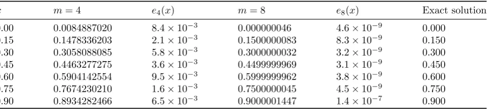
Table 4: Results of example 6.4in some special points.
x m= 4 e4(x) m= 8 e8(x) Exact solution
Table 5: Comparison between BPs method and block-pulse methods in example6.1.
method Mid-points,k= 32 Mid-points,k= 64 Ten points ,k= 32 Ten points ,k= 64
Direct method 3.3×10⁻³ 1.6×10⁻³ 5.9×10⁻³ 2.9×10⁻³ expansion-iterative rule 6.6×10⁻⁴ 1.9×10⁻⁴ 5.2×10⁻³ 2.6×10⁻³
m= 5 m= 8 m= 10
BPs method 7.70×10⁻⁴ 1.78×10⁻³ 2.62×10⁻³
Table 6: Comparison between BPs method and block-pulse methods in example6.3.
method Mid-points, k= 64 Mid-points,k= 128 Ten points ,k= 64 Ten points ,k= 128
Direct method 5.2×10⁻³ 2.6×10⁻³ 8.2×10⁻³ 4.1×10⁻³ expansion-iterative rule 4.9×10⁻⁴ 1.4×10⁻⁴ 6.5×10⁻³ 3.3×10⁻³
m= 5 m= 8 m= 12
BPs method 1.3×10⁻³ 2.5×10⁻⁴ 3.96×10⁻⁵
Table 7: Effect of noise on example7.1.
x m= 4 m= 4, ε= 0.01 m= 4, ε= 0.02 m= 4, ε= 0.03 Exact solution
0.0 0.00000 -0.00312608987 -0.00311339313 -0.003136934445 0.0000000 0.1 0.010000 0.01100083307 0.01097076095 0.01103789223 0.0100000 0.2 0.040000 0.03865110727 0.03854449585 0.03877979162 0.0400000 0.3 0.090000 0.08851961494 0.08827616242 0.08881386514 0.0900000 0.4 0.160000 0.15944664250 0.15900825960 0.1599768635 0.1600000 0.5 0.250000 0.24858913690 0.24790549840 0.2494161014 0.2500000 0.6 0.360000 0.35572905650 0.35475073140 0.3569125103 0.3600000 0.7 0.490000 0.48371881310 0.48238874880 0.4853278320 0.4900000 0.8 0.640000 0.63506381300 0.63331794130 0.6371759494 0.6400000 0.9 0.810000 0.80464208650 0.80242983060 0.8073183571 0.8100000 1.0 1.000000 0.96856101440 0.96589645720 0.9717837716 1.0000000
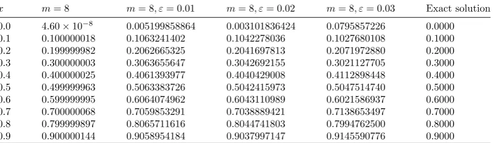
Table 8: Effect of noise on example7.2.
x m= 8 m= 8, ε= 0.01 m= 8, ε= 0.02 m= 8, ε= 0.03 Exact solution
0.0 4.60×10⁻⁸ 0.005199858864 0.003101836424 0.0795857226 0.0000 0.1 0.100000018 0.1063241402 0.1042278036 0.1027680108 0.1000 0.2 0.199999982 0.2062665325 0.2041697813 0.2071972880 0.2000 0.3 0.300000003 0.3063655647 0.3042692155 0.3021127705 0.3000 0.4 0.400000025 0.4061393977 0.4040429008 0.4112898448 0.4000 0.5 0.499999963 0.5063383726 0.5042415973 0.5047514740 0.5000 0.6 0.599999995 0.6064074962 0.6043110989 0.6021586937 0.6000 0.7 0.700000068 0.7059853291 0.7038889421 0.7138653497 0.7000 0.8 0.799999897 0.8065711616 0.8044741803 0.7994762500 0.8000 0.9 0.900000144 0.9058954184 0.9037997147 0.9145590776 0.9000
˜
ui,j =
0 if j < i and j > i+m
(m i)(
m j)
(2m i+j)
uj otherwise
for i, j= 0, ..., m.
Proof. Property P1 implies
Φm(x)ΦTm(x)u
= [
m
∑
j=0
(m
0
)(m
j
) (2m
j
) ujϕ∗j m
∑
j=0
(m
1
)(m
j
) (2m
j+1
) ujϕ∗j+1
... m
∑
j=0
(m
m
)(m
j
) (2m
m+j
Now,ith entry of the above matrix can be rewrit-ten as follows:
∑m j=0
(m i−1)(
m j)
( 2m j+i−1)
ujϕ∗j+i−1 =
[
i−1
z }| {
0· · ·0 (
m i−1)(
m 0)
(2m i−1)
u0 · · · (
m i−1)(
m m)
( 2m m+i−1)
um
m−i+1
z }| {
0· · ·0
]
Φ2m
5
Solution of integral equation
of the first kind
In this section, with respect to operational matri-ces and function approximation, integral equation converts to a system of equations.
5.1 Linear Volterra integral equation of the first kind
Consider the following Volterra integral equation of the first kind
f(x) =
∫ x
0
k(x, t)u(t)dt (5.4)
wheref andkare known butuis not. Moreover,
k(x, t) ∈ l2([0,1]×[0,1]) and f(t) ∈ l2([0,1]).
Approximating functions f, u and kwith respect to BPs gives
f(x) =FTΦm(x) = ΦTm(x)F
u(t) =UTΦm(t) = ΦTm(t)U
k(x, t)≃ΦTm(x)KΦm(t)
(5.5)
where the vectors F, U and matrix K are BPs coefficients of f(x), u(t) and k(x, t)respectively. Now, replacing (5.5) into the (5.4) gives:
FTΦm(x) =
∫ x
0
ΦTm(x)KΦm(t)ΦTm(t)U dt
= ΦTm(x)K
∫ x
0
Φm(t)ΦTm(t)U dt.
Using (4.3) follows:
FTΦm(x) = ΦTm(x)K
∫ x
0 ˜
UΦ2m(t)dt
= ΦTm(x)KU˜
∫ x
0
Φ2m(t)dt.
(5.6)
Using operational matrix of integrationM, in Eq. (5.6) gives:
FTΦm(x) = ΦTm(x)KU M˜ Φ2m(t)dt. (5.7)
Let U∗ = KU M T˜ m
2m, where U∗ is an (m+ 1)×
(m+ 1) matrix. Eq. (5.7) changes to:
FTΦm(x) = ΦTm(x)U∗Φm(x). (5.8)
Using Eq. (4.2) in (5.8) gives:
FTΦm(x) = ΦTm(x)U∗Φm(x) = ˆU∗ T
Φ2m(x).
Using decreasing transformation matrixT2mm , gives the final system:
¯
U =F,
where ¯UT = ˆU∗TT2mm.
5.2 Nonlinear Volterra integral equa-tion of the first kind
Consider the following nonlinear Volterra integral equation
f(x) =
∫ x
0
k(x, t)g(u(t))dt (5.9)
Put w(t) = g(u(t)) and Subsequently w(t) =
WTΦm(t) . WhereW is an unknown (m+1)-
vec-tor. Following the same procedure, final system is as follows: ¯W = F.Finally, u(x) = g−1(w(x)) is the desired solution.
6
Numerical examples
To show the efficiency of the proposed numerical method, we implement it on some Volterra inte-gral equations. For every example we use a ta-ble that shows exact solution, our approximation and absolute errors in some points. In the follow-ing examples, the absolute error is used to check the accuracy. The amount is far more than other computational errors like mean absolute error.
Example 6.1 u(x) =e−xis the exact solution of the following Volterra integral equation of the first kind xex = ∫x
0 ex+tu(t)dt. Numerical solution of
this equation and its errors are shown in table 1.
Example 6.2 Considerx=∫/x0(x+t−1)u(y)dt
with the exact solution u(x) = e−x. The table 2
shows approximation solutions, error and exact solution in some points.
Example 6.4 x=∫0x(x−t+ 1)e−u(t)dtis a
non-linear Volterra integral equation of the first kind with exact solution u(x) = x. Table 4 shows the exact solution, approximation solutions and abso-lute errors at some points.
Now, we compare our method with a direct method to solve Volterra integral equation of the rst kind using operational matrix with block-pulse functions [6] and an expansion-iterative method based on the block-pulse functions [21]. Consider example 6.1, Table 5 shows the mean-absolute errors for direct method and expansion-iterative method for two values of k, where k is the number of partitions of [0,1) also we can see absolute errors for some values ofm, for the same example.
Table6 shows the same errors for some different values ofkandmfor example6.3. Tables5and6 show our method is more accurate with respect to dimensions of the system. The final system in our method has smaller size than block-pulse meth-ods also, as another advantage ifk(x, x) = 0 then the block-pulse methods do not work and their final systems are incompatible but our method works correctly.
7
Stability
To demonstrate the stability of the method, we review effect of noise on data function. In other word, we replace f(x) by(1 +εp)f(x) in (5.4) or (5.9).wherepis a real random number between -1 and 1, and εis percent of noise.
Example 7.1 Consider the following Volterra
integral equation of the first kind 7 12x
4 =∫x ) (x+
t)u(t)dt with the exact solution u(x) =x2.
Suppose p is a random real number in (0,1)and
ε = 0.01,0.02,0.03. In table 7, we present ex-act solution, approximate and noisy solutions at some points.
Example 7.2 u(x) = x is the exact solution of the following Volterra integral equation of the first kind x=∫0x(x+t)u(t)dt.
Table 8 shows exact solution, approximate solu-tion and noisy solusolu-tions.
As a result of the tables, errors are proportional to the amount of noise.
8
Conclusion
In this article, we applied Bernsteins approxima-tion to approximate the soluapproxima-tion of linear and nonlinear Volterra integral equations of the first kind. In this method, we obtained some new op-erational matrices based on Bernstein polynomi-als. Our achieve results in this paper, show that our approach for solving Volterra integral equa-tions of the first kind is very effective, simple and stable. The answers are trusty and their accuracy are high and we this method can be can executed in a computer easily. The numerical examples support this claim. The method can be applied for integro-differential equations, integral equa-tions of the second and control problems.
References
[1] K. E. Atkinson, The Numerical Solu-tion of Integral EquaSolu-tions of the Sec-ond Kind,Cambridge University Press, Cam-bridge (1997).
[2] E.Babolian, L. Delves, An augmented Galerkin method for first kind Fredholm equations, IMA Journal of Applied Mathe-matics 24 ( 1979) 157-174.
[3] E. Babolian, R. Mokhtari, M. Salmani, Us-ing direct method for solvUs-ing variational problems via triangular orthogonal func-tions, Applied Mathematics and Computa-tion 191 (2007) 206-217.
[4] E. Babolian, H. Marzban, M. Salmani, Us-ing triangular orthogonal functions for solv-ing Fredholm integral equations of the sec-ond kind,Applied Mathematics and Compu-tation 201 (2008) 452-464.
[5] E. Babolian, Z. Masouri, S. Hatamzadeh-Varmazyar, Numerical solution of nonlinear Volterra Fredholm integro-differential equa-tions via direct method using triangular functions,Computers Mathematics with Ap-plications 58 (2009) 239-247.
[7] A. Bellour, E. Rawashdeh, Numerical solu-tion of first kind integral equasolu-tions by using Taylor polynomials, J. Inequal. Speci. Func 1 (2010) 23-29.
[8] P. J. Collins , Differential and integral equations, Oxford University Press, Oxford (2006).
[9] L. M. Delves, J. Walsh, Numerical solution of integral equations, Clarendon Press, Ox-ford, UK (1974).
[10] L. M. Delves, J.L. Mohamed, Computational methods for integral equations, Cambridge: Cambridge University Press (1985).
[11] M. A. Golberg, Numerical solution of in-tegral equations, Plenum Press, New York (1990).
[12] G. Hanna, J. Roumeliotis, A. Kucera, Col-location and Fredholm integral equations of the first kind,Journal of Inequalities in Pure and Applied Mathematics 6 (2005) 1-8.
[13] C. Hwang, Y. Shih, Optimal control of delay systems via block pulse functions, Journal of optimization theory and applications,45 (1985) 101-112.
[14] K. Joy, Bernstein polynomials, On-Line Ge-ometric Modeling Notes (2000).
[15] E. Kreyszig, Introductory functional anal-ysis with applications, Vol. 81, wiley, New York (1989).
[16] B. A. Lewis, On the numerical solution of Fredholm integral equations of the first kind, IMA Journal of Applied Mathematics 16 (1975) 207-220.
[17] K. Maleknejad, E. Hashemizadeh, R. Ez-zati, A new approach to the numerical solu-tion of Volterra integral equasolu-tions by using Bernsteins approximation, Communications in Nonlinear Science and Numerical Simula-tion 16 (2011) 647-655.
[18] K. Maleknejad, B. Basirat, E. Hashem-izadeh, A Bernstein operational matrix approach for solving a system of high order linear Volterra Fredholm integro-differential equations, Mathematical and Computer Modelling 55 (2012) 1363-1372.
[19] B. Mandal, S. Bhattacharya, Numerical so-lution of some classes of integral equations using Bernstein polynomials, Applied Math-ematics and computation 190 (2007) 1707-1716.
[20] F. L. Martinez, Some properties of two-dimensional Bernstein polynomials,Journal of approximation theory 59 (1989) 300-306.
[21] Z. Masouri, E. Babolian, S. Hatamzadeh-Varmazyar, An expansion iterative method for numerically solving Volterra integral equation of the first kind,Computers math-ematics with applications 59 (2010) 1491-1499.
[22] K. Parand, S. A. Kaviani, Application of the exact operational matrices based on the Bernstein polynomials, Journal of Mathe-matics and Computer Science 6 (2013) 36-59.
[23] P. Paraskevopoulos, P. Sparis, S. Mourout-sos, The Fourier series operational matrix of integration,International journal of systems science 16 (1985) 171-176.
[24] P. Paraskevopoulos, The operational matri-ces of integration and differentiation for the Fourier sine-cosine and exponential series, Automatic Control, IEEE Transactions on 32 (1987) 648-651.
[25] P. Paraskevopoulos, P. Sklavounos, G. C. Georgiou, The operational matrix of inte-gration for Bessel functions, Journal of the Franklin Institute 327 (1990) 329-341.
[26] G. M. Phillips, Interpolation and approxima-tion by polynomials, Vol. 14, Springer Sci-ence Business Media (2003).
[27] M. Rahman, Integral Equations and Their Applications, WIT Press, Southampton (2007).
[28] P. Sannuti, Analysis and synthesis of dy-namic systems via block-pulse functions, Proceedings of the Institution of Electrical Engineers 124 (1977) 569-571.
and Taylor expansion by collocation method, Appl. Math. Sci. 5 (2011) 685-696.
[30] A. Shirin, M. Islam, Numerical solu-tions of Fredholm integral equasolu-tions us-ing Bernstein polynomials, arXiv preprint arXiv:1309.6311 (2013).
[31] S. C. Tsay, T. T. Lee, Solutions of inte-gral equations via Taylor series, Interna-tional Journal of Control, 44 (1986) 701-709.
[32] W. Wang, A mechanical algorithm for solv-ing the Volterra integral equation, Applied mathematics and computation 172 (2006) 1323-1341.
[33] A. Wazwaz, Linear and nonlinear integral equations methods and applications,Higher Education Press, Beijing Heidelberg (2011).
[34] S. A. Yousefi, M. Behroozifar, Operational matrices of Bernstein polynomials and their applications, International Journal of Sys-tems Science 41 (2010) 709-716.
[35] S. A. Yousefi, M. Behroozifar, M. Dehghan, The operational matrices of Bernstein poly-nomials for solving the parabolic equation subject to specification of the mass, Jour-nal of computatioJour-nal and applied mathemat-ics 235 (2011) 5272-5283.
[36] S. A. Yousefi, M. Behroozifar, M. Dehghan, Numerical solution of the nonlinear age-structured population models by using the operational matrices of Bernstein polyno-mials, Applied Mathematical Modelling 36 (2012) 945-963.
Mohsen Mohamadi is Ph.D. Of applied mathematics and Faculty of Basic Science, Mathematics Department, Islamic Azad Uni-versity, Ayatolah Amoli Branch, Amol,Iran. Interested in Numer-ical Analysis, Integral Equations, and Differential equations.
Esmail Babolian - is Professor of applied mathematics and Fac-ulty of Mathematical sciences and computer, Kharazmy University, Tehran, Iran. Interested in numer-ical solution of functional Equa-tions, integral equaEqua-tions, differ-ential equations, numerical linear algebra and mathematical education.