Engineering
Volume 2, 2018, Pages 194–205
SUMO 2018- Simulating Autonomous and Intermodal Transport Systems
Multi-Level-Validation of Chinese traffic in the ChAoS
Framework
Marc Semrau
1, Jakob Erdmann
2, and Bernhard Friedrich
31
Volkswagen AG, Berliner Ring 2, 38440 Wolfsburg, Germany, [email protected]
2 Institute of Transportation Systems, German Aerospace Center
3 Institute of Transportation and Urban Engineering, 38108 Braunschweig, Germany
Abstract
This paper describes the validation of Chinese driver models in SUMO that enables a Chinese traffic simulation in the ChAoS framework. For validation a multi-level-concept is used, meaning that microscopic and macroscopic parameters are used. The results are discussed with respect to the characteristics of Chinese traffic, especially the improvements made by the sublane model.
Keywords: Heterogeneous traffic, Driver Model, Validation
1
Motivation and preliminary work
A new field of application for traffic simulation and driver modeling is continuously growing in importance, namely testing and developing driving functions1. Recently a lot of research has
been carried out in this area. Semrau et. al. developed, implemented [11,12] and calibrated [12] the so called ChAoS framework for testing driving functions in Chinese traffic. Fellendorf [5], Schamm et. al. [9] and Kaths et.al. [6] also presented concepts for testing driving function by using traffic simulations. All of them are so far missing one important last step: The validation. However, concepts for validation have been published before. In [8, 14] several validation concepts are presented and applied2. Detering suggest a methodology for data acquisition
in [2]. In contrast to Tomer et.al. [14] and Ni et.al. [8] he explicitly mentions the purpose of combining microscopic and macroscopic data. Without proving the validity of simulation models on both levels, the simulations cannot be used for testing driving functions. Precisely because those functions are based on the perception of surroundings. Accordingly the simulation models have to be validated on the level of driver interactions and traffic flow. Consequently we are going to deal with a Multi-Level-Validation-Concept and the results in this work.
1Those functions can be diverse. Adaptive cruise control is one example for an already established system,
while autopilot functions represent newly developed functions.
2
Validation concept
The importance of validation is well known in the research community. Without validating traffic or driver models and their calibration parameters the simulation results are not com-parable to reality and therefore not reliable. As stated before, this becomes even more true, when dealing with test and validation of driving functions. Therefore a lot of different methods for calibration and validation of traffic simulations have been established in the past years. The calibration process is described in [11,12], while this paper focuses on the validation part. Generally one can distinguish between three major strategies:
1. Macroscopic Validation: Here the validation is based on macroscopic data.
2. Microscopic Validation: Here the validation is based on microscopic data.
3. Multi-Level-Validation: Here the validation is based on both, microscopic and macroscopic data.
The macroscopic validation on it’s own only uses macroscopic parameters. Therefore it cannot describe car to car interaction directly and is not capable for the validation of driver parameters. Consequently it is not optimal for the focused use case of testing driving functions. In comparison driver parameters can be validated by using microscopic validation param-eters. Unfortunately, this approach by itself also has shortcomings. Since the macroscopic view is missing in this strategy it is not possible to validate the traffic flow as a whole. So the impacts of driving functions on the overall traffic cannot be analyzed. Consequently the Multi-Level-Validation is the only working strategy, when validating models for the test of driving functions on a large scale. Accordingly, we decided to use a methodology, based on the Multi-Level-Validation-Concept. A more detailed description of the three strategies and the developed method for the validation can be found in [10].
To the best of our knowledge this connection of microscopic and macroscopic validation level is not published in the way it is establish in [10]. To make it available to a bigger audience, the Multi-Level-Validation-Strategy Semrau used in [10] is summarized and presented in the following paragraphs. To do so the validation data basis is introduced, before the accomplished validation steps are described in detail. The paper ends with a benchmark of the developed and calibrated models and a short outlook on future work.
2.1
Data basis
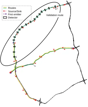
The validation data basis consists of real, as well as simulation data. The real traffic flow data is collected by more than 300 induction loops on elevated roads in Shanghai. Figure 1 illustrates the route and the induction loops (detectors), used for validation purpose. As typical for induction loops we monitored the number of cars (traffic volume), the average local speed and the traffic density. The measurement period is two weeks from Monday to Friday, between 6 am and 8 pm, so the morning and evening rush hour are covered, as well as the traffic during the day time. The time frame covered by this data, matches the data basis for the study described in [12]. Consequently the microscopic data of driver interactions from [12] is used in addition to the data of induction loops.
Routes Source/Sink First emitter Detector
1
17
Validation route
Figure 1: Simulation route with used induction loops
simulation. To ensure a representative distribution of drivers and the chance that no driver doubles we generated 2000 different drivers out of those parameter distributions.
2.2
Multi-Level-Validation
the comparability to other publications from the traffic domain, while the rmspe is widely applicable. The trend of macroscopic parameters is one more validation component. In [15] the trend of macroscopic parameter over time is rated by a graphical comparison. The same strategy will be used here.
The microscopic validation of driver parameters is carried out by comparing the statistical distributions in reality and simulation. The comparison of distributions in contrast to single values is necessary to take the variations of driver behavior into account. The focus is on lane change behavior, meaning the lateral and longitudinal behavior shortly before, during and shortly after lane changes. Consequently the minimal safety factors and the time gaps in the context of lane changing maneuvers are compared between simulation and reality. In addition, the minimal lateral gaps are analyzed to validate the china specificpushing behavior [11, 12]. both are also calibration parameters. Even though the validation data used here was not used for calibration we decided to include the resulting time gaps into the validation. Since this parameter is not a calibration parameter we can not only validate the correct calibration, but also the correct behavior of the implemented driver models. [10]
sectionValidation results The validation results of macroscopic and microscopic validation will be presented one after the other and the results are evaluated. In this context some limitations of the models will be discussed too. Finally the model extensions are benchmarked, by comparing them to the original driver model.
2.3
Macroscopic results
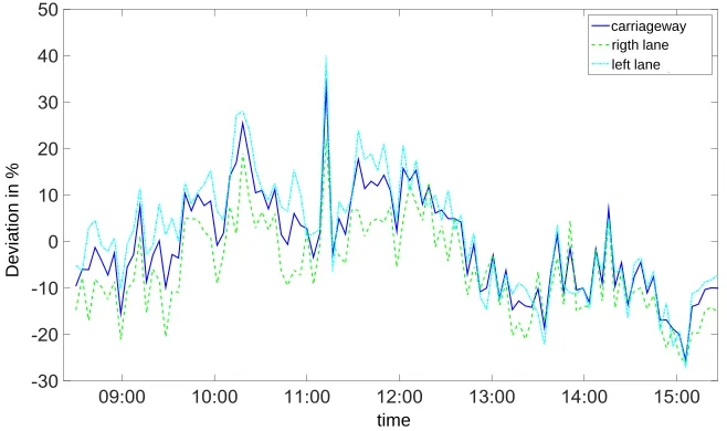
The first macroscopic validation step is to verify the quality of the lane assignment. To do so the errors of traffic volume from reality to simulation on the separate lanes are compared to the errors for the carriageway. As figure 2visualizes the errors are usually on the same scale,
De
via
tion
in
%
time
carriageway rigth lane left lane
Figure 2: Deviation of simulated traffic volume at detector 2
De
via
tion
in
%
time
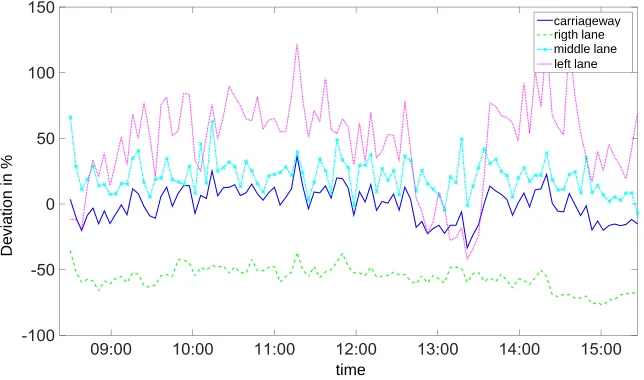
carriageway 1 rigth lane
left lane middle lane
Figure 3: Deviation of simulated traffic volume at detector 7
lane show errors that are bigger by the the factor ten, compared to the error for the carriageway. Since the errors of the rightmost and the leftmost lane are contrariwise, there seems to be a problem with the lane choosing algorithm. Figure 4 shows the reason pretty clearly. The
Figure 4: Concept of an additional lane from the right side
rightmost lane was just added to the roadway. Due to the calibrated waiting time [12] before changing lanes to the right, the drivers did not change before the induction loop is passed. Thus the error on the middle lane is small, whereas the errors are big on the left and right lane. This is caused by cars missing on the right lane, that appear on the left lane instead. So the error is explained by the special layout of the roadway and the induction loops.
However, this layout is not common in the data and the general concept of lane choosing was proved correct before. This induction loop will therefore be exclude for the validation of the models.
detectors. Evaluated according to HBS [1] the simulation models can therefore be seen as valid from a macroscopic point of view. One unexpected finding in [10, p.160] is that the errors seem to be independent from time and traffic density. This is unexpected, because the sublane model has strong influence on the capacity of the road.
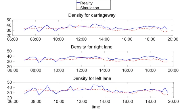
Shi et.al. indicate the traffic density as one more important parameter [13]. Analyzing the
time Density for carriageway
T
raf
fic
de
nsi
ty
in
veh
icl
es
/km
Reality Simulation
Density for right lane
Density for left lane
Figure 5: Traffic density per lane in reality and simulation
density, displayed in figure5, the overall trend of simulated and real data is similar. However there are some huge differences in single values.
This can have several reasons. Some of them have been discussed before and some more are going to be discussed in the following paragraph.
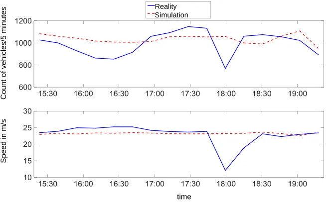
The first reason is a systematical error. The traffic density is not directly measured in the data, but calculated. To do so we have to approximate the average speed on the section, since the used induction loops can only measure the local speed [10]. The deviation between actual and estimated average speed is unknown. However, due to the relatively short distance of 300 to 500 meters between detectors we suppose it is acceptable. In figure6one can see an additional sources of error: Accidents on the road. Between 17:30 o’clock and 18 o’clock an accident happened during the real world test and one lane of the road was blocked. Due to the stochastic nature of the simulation, reproducing the exact time and location of that accident is not feasible. Hence the simulation is not configured to model accidents for this research work, even though the driver models are capable to show unsafe driving behavior and cause accidents. Consequently the capacity in the simulation is higher than on the real road. This kind of error cannot be filtered, due to the fact that detailed information on accidents is rare.
time
Sp
ee
d
in
m/
s
Co
un
t
of
veh
icl
es/5
min
ute
s Reality
Simulation
Figure 6: Effect of an accident on traffic volume and speed
such as floating car data. Additionally induction loops can have technical measurements errors in reality3, while they are free from these faults in the simulation. Since the deviations are
within the bounds prescribed for the GEH statistics, the above errors can be tolerated.
2.4
Microscopic results
In addition to the macroscopic validation results we present the microscopic results in this section. The first driver parameter we analyzed is the minimal safety factor. The safety factor is defined as:
s ssafe
(1)
With s being the actual gap andssafe the theoretical safe gap4.
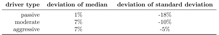
To do so we compare the distributions of safety factors of all three driver types. They are plotted in figure7. One can easily see the similarities between the real and the simulated distributions. One difference is that the simulated distributions are slightly moved to the right. This is probably caused by drivers that do not reach their minimal safety factor. For example because they did not experience a situation that made this necessary. A descriptive example: Driver that want to change their lane can do this for any safety factor bigger than their limit. Consequently the minimal safety factors are only reached in case of dense traffic and corresponding low distances between vehicles. In table 1 the quantitative deviations are shown.
One more finding is that the values for passive drivers differ less than for moderate or aggressive ones. This seems logical, since the smaller gaps of aggressive drivers are reached in
3Some cars may be counted twice, while some may be not counted at all.
4For the calculation of the safe gap please see the original model description[7], the SUMO wiki [3] or the
dens
ity
safety factor
passive moderate aggressive
Reality Simulation
Figure 7: Distribution of safety factors for all driver types
Table 1: Deviations of the safety factor distributions between simulation and reality
driver type deviation of median deviation of standard deviation
passive 1% -18%
moderate 7% -10%
aggressive 7% -5%
fewer situations, than the minimal values of passive drivers.
Compared to the median values the differences between reality and simulation for the stan-dard deviations are relatively big. The effect is well known, since simulations can never cover the variety of the reality completely. To prove statistical validity the Kolmogorov-Smirnov-Test is used. It can be proved5, that real and simulated values are based on the same statistical
population.
A similar strategy is used to validate the lane change behavior, especially the pushy behavior. The pushy behavior relates to virtual lane formation in dense traffic and was described in [11,12] To do so the minimal lateral distances6 during pushing situations is used.
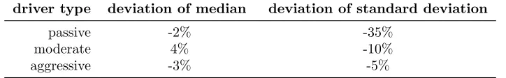
In figure 8 the distributions of the minimal lateral distances for the three driver types in reality and simulation are shown. To objectify the visual similarity the Kolmogorov-Smirnov-Test is also used here. The result is the same. The real and simulated distributions are based on the same statistical population. Table2summarizes the results.
The deviation of the median values is small and similar for all driver types. Whereas the standard deviations seem highly driver type depended. Passive drivers show the highest devi-ation between simuldevi-ation and reality. This is due to the effect of other driver types. Whenever
dens
ity
lateral gap in m
passive moderate aggressive
Reality Simulation
Figure 8: Distributions of the minimal lateral distances for all driver types
Table 2: Deviations of the lateral distance distributions between simulation and reality
driver type deviation of median deviation of standard deviation
passive -2% -35%
moderate 4% -10%
aggressive -3% -5%
moderate or aggressive drivers are evolved in a pushing maneuver, the lateral distances can be below the minimal ones of passive drivers. The resulting difference is smaller for moderate drivers and even less for aggressive drivers. The remaining deviation is caused by the variations within the class of aggressive drivers.
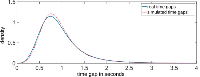
To this end we validated microscopic parameters, that are also part of the driver model itself. This is different for the last validation parameter, the time gaps. The time gaps in the context of lane changing have not been used for calibration purpose, but represent the result of the model behavior.
The distributions of time gaps in figure 9 are quite similar. The two logarithmic-normal-distributions are checked for equality with the Kolmogorov-Smirnov-Test again and equality could be proved on a level of 95 percent significance.
dens
ity
time gap in seconds
real time gaps simulated time gaps
Figure 9: Distributions of time gaps
standard deviation of reality and simulation. One more limitation is caused by the driver models themselves. They can only cover situations that were considered during modeling. Moreover some characteristics of driver models might work under certain conditions, but cause problems when experiencing unexpected situations. both aspects are discussed in detail in chapters 4 to 8 in [10].
2.5
Benchmark of sublane model
To benchmark the sublane model we are going to compare the performance with and without sublane model. Concerning the microscopic modeling the sublane model is the basis for sim-ulating pushing behavior. It enables drivers to drive between physical marked lanes, as long as space is sufficient. Moreover it allows a quasi continuous lateral dynamics and a pushing movement into blocked lanes. Therefore a microscopic valid simulation of Chinese traffic, with correct interaction between drivers, is not possible without this extension. By comparing the results of the macroscopic validation with and without extension we are going to prove the rele-vance of this behavior for the whole traffic flow. To get results of the original model we repeated the validation simulation with the exact same parameters and disabled all model extensions.
As a result the median of the rmspe of the traffic density on single lanes rises from 11.8 percent to 63.56 percent. For the whole carriageway it rises from 5.3 percent to 63.81 percent. Those values show the improvement pretty clearly. The main reason is the sublane model. It enables the pushing behavior that has strong influence on the traffic as a whole. One descriptive example is pushing at a motorway access [12]. In comparison to traffic without pushing, it is slowing down traffic on the motorway, while traffic on the ramp is more fluent. This seems to have significant influence on the following traffic. One more result the benchmark test shows is that the improvement is higher, when analyzing the whole carriageway.
We assume the sublane model, respectively the caused extension of the lane change model, is responsible for the deviation between the errors on the lanes and the carriageway too. Since there is nearly no difference without the sublane model. The higher complexity of the lane change decisions may require further research to get to an even better calibration.
3
Conclusion and future work
This paper presented a validation concept, that combines the validation on microscopic and macroscopic level. Moreover a Chinese traffic simulation is validated, using this concept. The validation proved the validity of the calibrated driver models for the simulation of traffic on Chinese elevated roads. Even though the results are pretty good they were discussed critically. Consequently not only validity is shown, but model boundaries and limitations were discussed. Those are mainly caused by the ideal perception of drivers and limitations of the routing algorithms. Finally the results were used to benchmark the developed model. The improvement is huge and demonstrates the necessity of the model extensions and a detailed calibration. Future work on validation concepts will probably focus on further traffic environments, further model extensions, like a perception model, to get rid of some more model boundaries and a further improvement concerning the calibration of sublane changes. Nevertheless the developed validation strategy is already applicable to these problems as well.
References
[1] Handbuch fuer die bemessung von strassenverkehrsanlagen hbs, 2015.
[2] Stefan Detering and Eckehard Schnieder. Two level approach for validation of microscopic simu-lation models. 0:18–22, 09 2009.
[3] Deutsches Zentrum fuer Luft und Raumfahrt. Sumo wiki definition of vehicles, vehicle types, and routes, 24.02.2018.
[4] Olga Feldman.The GEH measure and quality of the highway assignment models. 2012.
[5] Martin Fellendorf. Mikroskopische verkehrsflusssimulation – vom verkehrsmanagement zum au-tomatisierten fahren, 26.05.2016.
[6] Jakob Kaths and Sabine Krause. Integrated simulation of microscopic traffic flow and vehicle dynamics, 21.09.2016.
[7] Sven Bernd Kraus. Fahrverhaltensanalyse zur Parametrierung situationsadaptiver
Fahrzeugf¨uhrungssysteme. PhD thesis, Universit¨at M¨unchen, 2012.
[8] Daiheng Ni, John Leonard, Angshuman Guin, and Billy Williams. Systematic approach for
vali-dating traffic simulation models. Transportation Research Record: Journal of the Transportation
Research Board, (1876):20–31, 2004.
[9] Thomas Schamm, Ren´e Zofka, and Tobias B¨ar. Vehicle-in-the-loop: Innovative testing method for
cognitive vehicles, 2014.
[10] Marc Semrau.Untersuchung zur Modellierung von chinesischem Fahrverhalten auf Autobahnen f¨ur
den Test pilotierter Fahrfunktion: in Ver¨offentlichung. Auto Uni Schriftenreihe. Springer, 2018.
[11] Marc Semrau, Jakob Erdmann, Bernhard Friedrich, and Waldmann Ren´e. Simulation framework
for testing adas in chinese traffic situations. SUMO Proceedings, 2016:103–114.
[12] Marc Semrau, Jakob Erdmann, Jens Rieken, and Bernhard Friedrich. Modelling and calibrating
situation adaptive lane changing and merging behavior on chinese elevated roads.SUMO
Proceed-ings, pages 15–27, 2017.
[13] Bin Shi, Li Xu, Jie Hu, Yun Tang, Hong Jiang, Wuqiang Meng, and Hui Liu. Evaluating driving
styles by normalizing driving behavior based on personalized driver modeling.IEEE Transactions
on Systems, Man, and Cybernetics: Systems, 45(12):1502–1508, 2015.
[14] Tomer Toledo and Haris Koutsopoulos. Statistical validation of traffic simulation models.
Trans-portation Research Record: Journal of the TransTrans-portation Research Board, 1876:142–150, 2004.
[15] Stefan Witte. Simulationsuntersuchnungen zum Einfluß von Fahrverhalten und technischen