__________
* Corresponding author
E-mail addresses:[email protected](A.Shahamat) DOI: 10.22059/eoge.2019.271073.1040
118
Determination of optimal gravity mission for the coseismic earthquake signals
detection
Abolfazl Shahamat
Department ofSurveyingEngineering, Marand Technical College, University of Tabriz, Tabriz, Iran
Article history:
Received:25March2018, Received in revised form:10November2018, Accepted:13November2018 ABSTRACT
The gravity field of the earth has temporal variations and our instruments are unfortunately defective and imperfect to measure that. Therefore, our knowledge of the gravity field of the earth is not complete. After launching satellite gravity missions, gravity data has been collected with a remarkable quality. One of the changes that takes place under the surface of the earth is a mass movement, which occurs as a result of several earthquakes. In the case of using multiple satellites, we might be able to achieve an additional amplification of the gravity signal through inter-satellite tracking between two low orbits. In this paper, five scenarios were simulated and compared with one another. For a better comparison, five different simulated faults in three deferent positions were considered to the orbit simulation scenarios. We also used the simulated data of both the earthquake and orbit propagation scenarios. In addition, we added normal noises in satellites orbit propagation step. Then, the 1964 earthquake caused by the Alaska () fault was investigated as a case study. For the Alaska fault, the seawater effect was considered, as well. The results indicated that the observations made by Helix and Pendulum scenarios had a better susceptibility to earthquake signals, and GRACE and GRACE-FO had the least susceptibility. Therefore, the radial track is considered to be an important part of observations as well as cross-track and along-track to be in the next order, respectively.
S
KEYWORDS
Earthquake Signal Gravity Changing
Satellite Gravity Coseismic
Numerical Simulation
1. Introduction
Strong earthquakes usually occur close to faults and pose a big threat to communities. The observation of earthquake-induced gravity changes can be an indirect way of measuring a seismic deformation. Earthquakes are natural disasters and they can not only be extremely destructive but also increase the fatality rate. On the other hand, they are good scientific sources for scholars of Geodesy, Geodynamic, Geophysics and Geology to conduct new investigations. This can provide the scientists with an opportunity of studying the response of the solid earth to a tectonic loading. Since large earthquakes lead to massive movements of the crust and the mantle. The resulted uplifting or subsiding imply the redistribution of mass and finally cause changes in the gravity field. Among the researches, the study of coseismic deformation is one of the most important subjects. Several studies have been
undertaken to inspect a coseismic deformation in a half-space earth model by (Steketee, 1958),(Okada, 1985). They have presented analytical views for calculating the surface displacement, tilt, and strain resulting from various dislocations (Sun et al., 2010). Okada (1985) offered a complete set of analytical formulae to calculate these geodetic deformations by providing a review on the previous studies. Closed-form expressions were also proposed by
(Okubo, 1992) to describe the potential and gravity changes
resulted from dislocations. Due to their mathematical simplicity, these dislocation theories have been applied widely to study seismic faults (Sun et al., 2010).
Obviously, the temporal changes of the Earth’s gravity field can be observed on a global scale with low–low satellite-to-satellite tracking (SST) missions. Therefore, for a
111 better understanding of the faults, the seismicity mechanisms
and physics of the interior of the earth should be studied. In order to do so, we should improve our knowledge of the earth interior and its gravity field. Since there are many instrumental limitations and the impossibility of collecting data from the entire surface of Earth, the knowledge of the Earth’s gravity field is incomplete. Besides, periodic, global, and homogeneous data collection procedures are necessary for more fruitful studies. Therefore, we need satellites with better scenarios and lower heights. For this purpose, three satellites named CHAMP (CHAllenging Mini satellite Payload) in 2000, GRACE (Gravity Recovery and Climate Experiment) in 2002, and GOCE (Gravity recovery and steady-state Ocean Circulation Explorer) in 2004 were lunched (Sharifi et al., 2017). All of the scenarios had low and nearly a polar orbit. They continuously collected data and in a three-dimensional format. All of these scenarios could separate non-gravitational from of the gravitational signal parts. In the scenarios with pair satellites (like GRACE), inter-satellite distance changes are tracked and in the scenarios with a single satellite (like GOCE), the gravity gradiometry is checked. Accordingly, the final gravity signal is achieved (Rummel et al., 2002). The development of space geodetic techniques such as the satellite gravity missions have favored the detection of coseismic gravity changes from space. The coseismic gravity change caused by the 2004 Sumatra earthquake was detected by GRACE (Sun & Okubo,
2004, Han et al., 2006). The gravity changes caused by the
earthquake were calculated and interpreted by using a very simple method based on a half-space earth model (Han et al., 2006).
During the past two decades, satellite gravity missions (CHAMP, GRACE and GOCE) increased the accuracy, spatial resolution, and temporal resolution of the Earth’s gravity potential models (Elsaka et al., 2014). In the future, we may have access to improved data if better scenarios are launched in different configurations. In order to obtain optimum scenarios, different studies have been published during the last decades and they are all included in (Elsaka et
al., 2014). They have revealed a substantial increase in the
accuracy and sensitivity. After the Sumatra-Andaman earthquake and the analysis of GRACE data, the application of GRACE data to detect coseismic effects was found to be feasible [e.g.,
Han et al., 2006
; Chen et al., 2007; Han et al., 2010;Heki & Matsuo, 2010; Han et al., 2011; Kobayashi et al., 2011;Matsuo & Heki, 2011; Cambiotti & Sabadini, 2012; Wang et al., 2012a; Zhou et al., 2012; Han et al., 2013; Daiet al., 2014]. The modern geodetic techniques will enable us
to have a better detection of the coseismic deformations such as displacement, gravity changes, etc. [e.g., Han et al., 2006; Chang & Chao, 2011; Hayes, 2011; Ito et al., 2011;Kobayashi et al., 2011; Sato et al., 2011; Shao et al., 2011; Suito et al., 2011; Sleep, 2012; Suzuki et al., 2012;
Wang, 2012; Wang et al., 2012b; Li & Shen, 2015].
The main focus of this paper is on gravity satellites that sense earthquake signals in the best quality via alternative configuration scenarios applied in future gravimetric satellite missions. Full-scale simulations of various mission scenarios
covering GRACE, GRACE-FO, Cartwheel, pendulum and Helix were performed. In this work, one more month was added to the simulated time span to analyze the simulated earthquake signals. This research investigates the sensitivity of satellite gravity scenarios to gravity changes caused by three different faults spread on the world map as the case study. The results of this study are tested on five different faults on the Gauss Grid network. This has been calculated by Geometry-based Okubo model. The paper is organized into the following sections: Section 2 reviews the methodology. Then in Section 3, the simulated measurements are described and earthquake simulations are included. The results are shown in Section 4. The summery and a brief conclusion of the paper are provided in the final section.
2. Methodology
2.1 Determination of gravity changes based on earthquake models
At first, the gravity changes are calculated by the Okubo’s model. This model is used for a range of grounds where the sphericity can be ignored. Using the Okubo’s model, one can get the gravity disturbance for every geometry type of earthquakes. That is why this model has been implemented in this study. The total gravity changes on the free surface are calculated due to the simulation of earthquakes. Interested readers can refer to (Okubo, 1992)for more details.
Afterward, the range of coordinates is mapped in the spherical system. The gravitational field difference before and after an earthquake can be computed and derived from
(Rummel et al., 2002);
∆𝑉(𝑟,,) =𝐺𝑀𝑟 (∑𝑙𝑚𝑎𝑥(𝑅𝑟)𝑙
𝑙=2 ∑𝑙𝑚=0(∆𝐶𝑙𝑚cos 𝑚+
∆𝑆𝑙𝑚sin 𝑚)𝑃𝑙𝑚(𝑐𝑜𝑠ɵ)) (1)
(𝑟,,) are radius, longitude, and latitude of spherical geocentric coordinates, respectively. 𝐺𝑀 is the product of gravitational constant and mass of the Earth, and 𝑅 is the radius of earth equator; 𝐶𝑙𝑚, 𝑆𝑙𝑚 are coefficients of the spherical harmonic function; 𝑃𝑙𝑚(𝑐𝑜𝑠ɵ) is fully normalized
Legendre function of order m and degree l. 2.2.Selection of missions and parameters of orbit
121 satellite-to-satellite tracking observations with a near-polar
inclination are the inter-satellite distance and the scalar relative velocity. In GRACE and GRACE-FO, the observations are nearly only in the North-South direction and streaks appear along the meridians in the monthly GRACE solutions (Sharifi et al., 2007). These streaks are caused because the observations suffer from the weakness of sensitivity along the line-of-sight [e.g. (Tapley et al., 2004)].
(Sneeuw et al., 2008) have demonstrated that this problem
can be alleviated if there is a radial and/or cross-track gravitational signal in the SST observation. To solve this problem, we can design a scenario with a rotating baseline in the satellites’ local frame.
(Sharifi et al., 2007) introduced four generic types of
Low-Earth Formations (LEF). We refer the interested reader
to (Sharifi et al., 2007)for more details. The vectoral gradient
difference in gravitational attraction between two satellites projected along the Line Of Sight (LOS) is derived by Liu (Liu, 2008):
2
.
r e
r
(2)The left part (∆𝐫̈. 𝐞) shows the gravitational attraction difference between the two satellites projected along the LOS while the right part consists of the HL-and LL-SST measurements.
For every type of formations, each term on the observation has different value and as a result, has various contributions to the entire observation. Furthermore, the quality of observations depends on the gravity signal taken by the type of formation (Sharifi et al., 2007). This equation is the basic relation between KBR system observations and unknown gravity fields. Here ρ is the distance between two satellites, ρ̇ is the distance range-rate and ρ̈ is acceleration. e is the unit vector of the relative position. ∆r̈ is the relative acceleration between these two satellites. KBR observations are based on the measurement of the rate of the changes in the distance between two satellites. The distance between two satellites is achieved by GPS observations. The acceleration range between two satellites is derived from numerical differentiation of ρ̇. For more details see (Case et
al., 2002). All considered scenarios in this study use all
parameters and conditions of (Elsaka et al., 2014). The scenarios that have a greater signal to noise ratio are more suitable for observations. Now if our observations include cross-track signals, our observations are sensitive in an East-West direction. This may be helpful in de-aliasing the signals. Moreover, the radial components lead to nearly homogeneous results in the Helix configuration (Sharifi et
al., 2007). Thus, the inherent weakness and the non-isotropic
behavior of such scenarios can be solved. The radial component is the main source of gravity field information; therefore, this signal is very valuable in satellite gravity observations (Sneeuw, 2000).The GRACE and GRACE-FO observations have only along-track signals; therefore, their results are the poorest while the Helix mission presents the best signals on all three contributed components (Sneeuw &
Schaub, 2005). The Pendulum mission observations do not
have cross-track signals and contain only along-track and radial-track. The Cartwheel observations contains horizontal
information. Its signals have only along-track and cross-track and it does not have any radial-track signals. This explains why it does not gain the performance level of the Pendulum mission. For more information, the reader can refer to
(Sharifi et al., 2007)and (Elsaka et al., 2014). Although the
above-expressed opinions seem logical, but they cannot be a reason to detect all kinds of signals. For example, considering that Cartwheel has a cross-track, it can sense earthquakes with Strike= 0°. On one hand, they can sense all signals in their resolution interval but cannot detect them. On the other hand, each variation and event have their mechanism and cannot be claimed to be achieved with a more accurate mission.
2.3. Time-variable gravity signals
The mass redistributions like ocean circulations, atmospheric effects, and ocean (and crust) tides might change the gravity of earth (Han et al., 2006). Separating the effect of the earthquake gravity anomaly from the other effects could be considered as a difficulty, but the periodic behavior of the predominant temporal gravity variation could help us to separate them from permanent gravity changes such as earthquakes. To remove undesirable periodic signals, one could take differences of the gravity solutions from the same months in various years. This can remove the noticeable periodic gravity variations that are driven by temporal variations with a sub-annual and seasonal period. In a nutshell, the bulk data gathered before and after the earthquake could further increase the signal-to-noise ratio in the discerned satellite gravity anomaly due to the perpetual mass transfer (Han et al., 2006).
Because of the aim of this study (sensitivity of scenarios to earthquake signals), we used simulated data. The addition and subtraction of this kind of effects were not a focal point in this research. As the GRACE satellite is still the only couple satellite launched, the calculations process was applied to these scenarios. On the other hand, the data was not accessible as well. However, the geophysical signals such as atmospheric, oceanic and hydrological effects, which have time variable gravity, change signals well resolved with the following procedure for this scenario: Some of the well-known time-variable gravity signals observed by the GRACE satellites, including tides (of the solid earth, ocean, atmosphere, and pole) and atmospheric and ocean barotropic mass variations, have been removed from satellite observations using a priori models. Although the solid-earth mass transport induced by earthquakes is abrupt and permanent, climate-related signals such as hydrological and ocean mass fluxes are periodic, with primarily seasonal and possibly inter annual or longer time scales. In order to eliminate signals other than those associated with an earthquake, we took the differences of gravity solutions (from the same months in various years), using dominant gravity variations driven by seasonal changes. By using multiple months of data, we can further enhance the tectonic signal-to-noise ratio (SNR) in the GRACE gravity solutions
(Han et al., 2006).
121 was used to compute the effect of non-seismic signals in the
data after the earthquake, assuming no significant changes occurred from non- seismic sources during one month (Han
et al., 2011). Therefore, the reference global mass
distribution computed from one -month worth of the satellite data immediately before the earthquake, could be subtracted from computed gravity disturbance within occurred earthquake periods in case of the real satellite computed gravity disturbance.
2.4. Ocean mass redistribution
When earthquake draws near the ocean coast, relative sea level changes causes deformation of the ocean floor, therefore, making mass redistribution of water have a significant effect on the gravity field [e.g., Heki and Matsuo,
2010;Broerse et al., 2014)]. Hence, the sea water correction
becomes significant. Of course, if the earthquake position is far from the sea, the water correction is not necessary and the signals will be bigger and stronger. Interested readers can refer to [e.g., Broerse et al., 2011; Broerse et al., 2014; Heki
& Matsuo, 2010; Li et al., 2016] for more details. Here, we
do not use the ocean compression on Figure 3 because the selected faults are simulated with different parameters. As
indicated earlier, the aim of this article is to investigate the impact of gravity changes resulting from earthquakes on the already mentioned scenarios. Therefore, although the sea compression reduces gravity changes signals, it will not have an effect on how to get signals. Nevertheless, Figure 6 shows that due to the use of the real fault, we considered the ocean compassion.
3. Analysis of simulated data
3.1 Satellite gravity scenarios
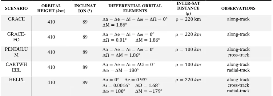
In this study, the GRACE, GRACE-FO, pendulum, Cartwheel and Helix (LISA-like) formations have been selected as basic mission scenarios. In this paper, it has been tried to simulate the same circumstances and the start position for the first satellites are the same. However, other parameters for satellite orbits are different because we wanted to create different scenarios. The characteristics of satellite orbits are presented in Table 1.
Table 1. Satellite Orbits characteristics
SCENARIO ORBITAL
HEIGHT (𝒌𝒎)
INCLINAT ION ()
DIFFERENTIAL ORBITAL ELEMENTS
INTER-SAT DISTANCE
()
OBSERVATIONS
GRACE
410 89 a =M = 1.86e =i === 0 = 220 km along-track
GRACE-FO 410 89
a =e =i == 0
= 0.01 M = 1.86 = 220 𝑘𝑚 along-track
PENDULU
M 410 89
a =e =i == 0
=M = 1.86 = 100 𝑘𝑚 along-track cross-track
CARTWH
EEL 410 89
a =e =i == 0
=M = 180 = 100 𝑘𝑚 along-track radial-track
HELIX
410 89 a = 0i = 0.0016 e = 0.93 = 1.68 = 180 M = −179
= 220 𝑘𝑚 along-track
cross-track radial-track
Table 2. Simulation Setting (Sharifi & Shahamat, 2017) Force fields models
Gravity of the central body GGM03S released by CSR on2007 Reference frames and transformation
Earth Center Earth Fixed (ECEF) frame ITRF 2008
Geographical coordinates GRS80 (semi-major axis a=6378137.0 m, flattening =1/298.257222101) Geocentric Celestial Reference Frame
(GCRF)
Only GAST corrected reference
Earth rotation Simple GAST ( GAST = GAST0+ ωt)
The GRACE mission results have revealed that ground track coverage via the choice of orbit repeat modes can have a significant effect on the quality of the gravity retrievals.
(Wagner et al., 2006) showed that large gaps that are created
because of short repeat cycles degrade GRACE results remarkably. Accordingly, in this paper, the total simulation period is set to 31 days (one consecutive month). To find out how this number is found and chosen refer to (Wagner et al., 2006), (Visser et al., 2010) and (Wiese et al., 2012). The
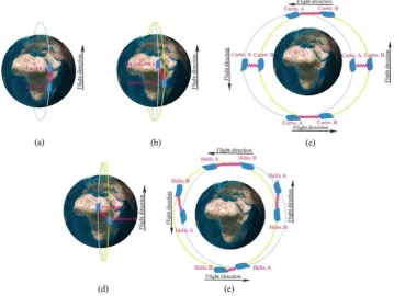
122 have displayed different constellations in Figure 1. In these
scenarios, the distance between two satellites is always changing. However, the changes vary depending on the type of satellites. For example, in GRACE, this changing is minimal and is the main factor for calculating the gravitational anomaly. In these scenarios, the distance between two satellites is always changing. However, the changes vary depending on the type of satellites. For example, in GRACE, this changing is minimal and is the main factor for calculating the gravitational anomaly. 3.2. The fault of earthquakes
In this section, three different areas with different coordinate positions are selected to consider the impact of
mass change location on different scenarios. Hence, a signal might be more sensitive in one position to receive the changes rather than the other position. For this purpose and for a better investigation of the purpose of the study, three different areas were selected (Table 3). Furthermore, at each location, 5 different fault modes were chosen to be considered beside the influence of positions, the influence of different parameters of fault on scenarios, and the sensitivity of signal receiving by scenarios (Table 4). In these selections, it is assumed that there is the possibility of such faults. The selective faults might not be the real ones; however, to investigate the case, such assumptions are inevitable.
Figure 1. The investigated FGM configurations, GRACE-reference (top-left), alternative GRACE Follow-on (top-middle), Cartwheel (top-right), Pendulum (bottom-left), Helix (bottom-right) (Elsaka et al., 2014).
3.3. Noise and Smoothing data
To reduce the contribution of noisy short-wave length components of the gravity field solutions, spatial averaging, or smoothing of satellite data are necessary. The filter methods not only remove part of the noise at short wavelengths but also remove longitudinal patterns like that of the coseismic gravity change pattern of the earthquake. Here we smoothed the GRACE and GRACE-FO data with a 300 km Gaussian filter and the Cartwheel, Pendulum, and Helix data smoothed with a 250 km, 200 km and 200 km respectively. Moreover, we used only 120 coefficients in the recovery of the orbits. Then, each gravity field was comprised of a set of spherical harmonics (Stokes)
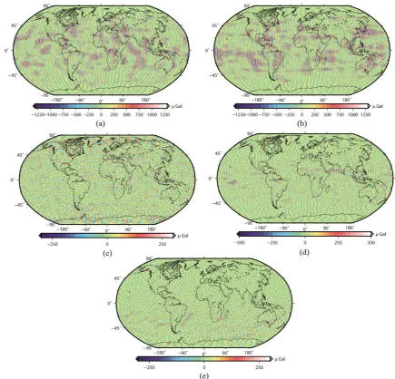
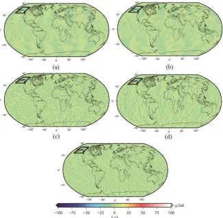
121 Figure 2. Co-seismic gravity changes maps of simulated Alaska earthquake (a) GRACE, (b) GRACE-FO, (c) Cartwheel, (d)
Pendulum and (e) Helixdata
To achieve that, we computed the co-seismic gravity changes due to the earthquake simulated by specified fault parameters in a half-space model. Then, the computed gravity changes were added to the computed reference gravity from EGM96. Finally, the spherical harmonics coefficients were estimated from the collected gravity data. It is worth to mention that the recovered coefficients include the effects of the earthquake vis-a-vis the reference filed. Then, the satellite orbit was reproduced by using these coefficients. After generating the orbit, we added white noise to the orbit considering all measurement precisions according to (Zheng et al., 2015) assumptions highlighted in Table 5. Afterward, the SH coefficients were recovered by the acceleration approach from the computed orbits (see [e.g., (Liu, 2008)]). After deducting the reference model from the recovered coefficients, the goal gravity disturbances were computed showing the effect of the earthquake on the spatial gravity disturbance map.
4. Results
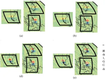
As already mentioned, in this paper, five scenarios are used including GRACE, GRACE-FO, Cartwheel, Pendulum, and Helix. In order to analyze the ability of these scenarios, three sporadically different positions were considered (Table 3). Moreover, for each position, five different faults (Table 4) were simulated, although the readers might claim that there are no such faults in those areas. Those faults were selected just for study of the influence of the same fault in different areas in fair judgment on the different scenarios data. Figure 3 and 4 shows the co-seismic gravity changes due to the earthquake created by fault 1 (Table 4) in different positions (Table 3).
Table 3. Characteristics of selection hypothetical positions
Latitude Longitude
Position 1 40 N 140 E
Position 2 45 S 73 W
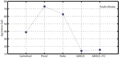
121 The obtained max signal of co-seismic gravity changes in the
spatial domain (peak-to-peak) is depicted in the Figure 5. Every figure shows one position (Specified in Table 3) and each graph is drawn in any figure indicates specific fault (indicated in Table 4). Ultimately, the co-seismic gravity changes caused by the Alaska (1964) earthquake through the considered scenarios are displayed in Figure 6. Also, the obtained max signal of co-seismic gravity changes to this fault is displayed in Figure 7. The graphs are shown that the scenarios which have radial track observation have a good sensitivity to earthquake signals.
5. Conclusion
In the future, satellite missions can be able to solve much more problems in the gravity field. The GRACE mission gave us good results as the first experience. Nevertheless, its observations have only along-track signals. Therefore, it seems that because of the satellite motion and the type of observations, a large part of signals is polluted to noise and because of filtering, a large part of signals is inevitably removed. If our formations involve a cross-track or radial components, they should have the same features as a GRACE-type leader-follower configuration. As seen in Figure 5, coseismic signals have different effects at different scenarios and different parameters. In general, the graphs show that the scenarios that have radial track observations have a good sensitivity to earthquake signals. In the best
situation, if observations include at least either of cross-track or along-track together with a radial one, the results will noticeably improve. The observations in such formations are significantly richer in gravitational content. This condition is not, of course, limited to coseismic signals detection.
Table 4. Five different selected faults
Length Width Depth Dip Strike Pake Slip
Fault 1 600 200 35 0 90 0 10
Fault 2 400 100 35 0 90 0 6
Fault 3 600 200 35 90 90 0 10
Fault 4 600 200 35 0 0 0 10
Fault 5 600 200 35 0 90 90 10
Table 5. Payload of the current GRACE satellite gravity mission and its measurement precision (Zheng et al. (2015))
Measurement precision
Orbital position: 10-2 m
Orbital velocity: 10-5 m/s
Table 6. The Alaska fault parameters (http://USGS.com)
STRIKE DEPTH DIP LENGTH WIDTH RAKE SLIP
Alaska 270 25 9 600 200 90 10
Table 7. The Alaska fault epicenter (http://USGS.com) Epicenter
Earthquake Latitude Longitude Mw
121 Figure 3. Co-seismic gravity changes in the spatial domain (µGal) in position 1,2, 3 and Fault 1 simulated by (a) GRACE, (b)
GRACE-FO, (c) Cartwheel, (d) Pendulum, and (e) Helix data
(a) (b) (c)
(d) (e)
[[[[
121 Figure 5. The obtained max signal of co-seismic gravity changes in the spatial domain (µGal) in position 1 and five simulated
faults. (a) Fault 1, (b) Fault 2, (c) Fault 3, (d) Fault 4, and (e) Fault 5
121 Figure 7. The obtained max signal of co-seismic gravity changes in the spatial domain (µGal) by the Alaska simulated fault References
Broerse, D. B. T., Vermeersen, L. L. A., Riva, R. E. M., & Van der Wal, W. (2011). Ocean contribution to co-seismic crustal deformation and geoid anomalies: application to the 2004 December 26 Sumatra– Andaman earthquake. Earth and Planetary Science Letters, 305(3-4), 341-349.
Broerse, T., Riva, R., & Vermeersen, B. (2014). Ocean contribution to seismic gravity changes: the sea level equation for seismic perturbations revisited. Geophysical Journal International, 199(2), 1094-1109. Cambiotti, G., & Sabadini, R. (2012). A source model for the
great 2011 Tohoku earthquake (Mw= 9.1) from inversion of GRACE gravity data. Earth and Planetary Science Letters, 335, 72-79.
Case, K., Kruizinga, G., & Wu, S. (2002). GRACE level 1B data product user handbook. JPL Publication D-22027. Chang, E. T., & Chao, B. F. (2011). Co-seismic surface deformation of the 2011 off the Pacific coast of Tohoku Earthquake: Spatio-temporal EOF analysis of GPS data. Earth, planets and space, 63(7), 25.
Chen, J. L., Wilson, C. R., Tapley, B. D., & Grand, S. (2007). GRACE detects coseismic and postseismic deformation from the Sumatra‐ Andaman earthquake. Geophysical Research Letters, 34(13).
Dai, C., Shum, C. K., Wang, R., Wang, L., Guo, J., Shang, K., & Tapley, B. (2014). Improved constraints on seismic source parameters of the 2011 Tohoku earthquake from GRACE gravity and gravity gradient changes. Geophysical Research Letters, 41(6), 1929-1936.
Elsaka, B., Raimondo, J. C., Brieden, P., Reubelt, T., Kusche, J., Flechtner, F., ... & Müller, J. (2014). Comparing seven candidate mission configurations for temporal gravity field retrieval through full-scale numerical simulation. Journal of Geodesy, 88(1), 31-43.
Han, S. C., Shum, C. K., Bevis, M., Ji, C., & Kuo, C. Y. (2006). Crustal dilatation observed by GRACE after the 2004 Sumatra-Andaman earthquake. Science, 313(5787), 658-662.
Han, S. C., Riva, R., Sauber, J., & Okal, E. (2013). Source parameter inversion for recent great earthquakes from a decade‐ long observation of global gravity fields. Journal of Geophysical Research: Solid Earth, 118(3), 1240-1267.
Han, S. C., Sauber, J., & Luthcke, S. (2010). Regional gravity decrease after the 2010 Maule (Chile) earthquake
indicates large‐ scale mass redistribution. Geophysical Research Letters, 37(23).
Han, S. C., Sauber, J., & Riva, R. (2011). Contribution of satellite gravimetry to understanding seismic source processes of the 2011 Tohoku‐ Oki earthquake. Geophysical Research Letters, 38(24).
Hayes, G. P. (2011). Rapid source characterization of the 2011 M w 9.0 off the Pacific coast of Tohoku earthquake. Earth, planets and space, 63(7), 4.
Heki, K., & Matsuo, K. (2010). Coseismic gravity changes of the 2010 earthquake in central Chile from satellite gravimetry. Geophysical Research Letters, 37(24). Ito, T., Ozawa, K., Watanabe, T., & Sagiya, T. (2011). Slip
distribution of the 2011 off the Pacific coast of Tohoku Earthquake inferred from geodetic data. Earth, planets and space, 63(7), 21.
Kobayashi, T., Tobita, M., Nishimura, T., Suzuki, A., Noguchi, Y., & Yamanaka, M. (2011). Crustal deformation map for the 2011 off the Pacific coast of Tohoku Earthquake, detected by InSAR analysis combined with GEONET data. Earth, planets and space, 63(7), 20.
Li, J., Chen, J. L., & Wilson, C. R. (2016). Topographic effects on coseismic gravity change for the 2011 Tohoku‐ Oki earthquake and comparison with GRACE. Journal of Geophysical Research: Solid Earth, 121(7), 5509-5537.
Li, J., & Shen, W. B. (2015). Monthly GRACE detection of coseismic gravity change associated with 2011 Tohoku-Oki earthquake using northern gradient approach. Earth, Planets and Space, 67(1), 29.
Liu, X. (2008). Global gravity field recovery from satellite-to-satellite tracking data with the acceleration approach, Nederlandse Commissie voor Geodesie.
Matsuo, K., & Heki, K. (2011). Coseismic gravity changes of the 2011 Tohoku‐ Oki earthquake from satellite gravimetry. Geophysical Research Letters, 38(7). Okada, Y. (1985). Surface deformation due to shear and
tensile faults in a half-space. Bulletin of the seismological society of America, 75(4), 1135-1154. Okubo, S. (1992). Gravity and potential changes due to shear
and tensile faults in a half‐ space. Journal of Geophysical Research: Solid Earth, 97(B5), 7137-7144.
121 Sato, M., Ishikawa, T., Ujihara, N., Yoshida, S., Fujita, M.,
Mochizuki, M., & Asada, A. (2011). Displacement above the hypocenter of the 2011 Tohoku-Oki earthquake. Science, 332(6036), 1395-1395.
Shao, G., Li, X., Ji, C., & Maeda, T. (2011). Focal mechanism and slip history of the 2011 M w 9.1 off the Pacific coast of Tohoku Earthquake, constrained with teleseismic body and surface waves. Earth, planets and space, 63(7), 9.
Sharifi, M., Sneeuw, N., & Keller, W. (2007, June). Gravity recovery capability of four generic satellite formations. In Proc. Symp.“Gravity Field of the Earth”, General Command of Mapping (pp. 211-216).
Sharifi, M. A., & Shahamat, A. (2017). Detection of co-seismic earthquake gravity field signals using GRACE-like mission simulations. Advances in Space Research, 59(10), 2623-2635.
Sleep, N. H. (2012). Constraint on the recurrence of great outer-rise earthquakes from seafloor bathymetry. Earth, Planets and Space, 64, 1245-1246.
Sneeuw, N. (2000). A semi-analytical approach to gravity field analysis from satellite observations (Doctoral dissertation, Technische Universität München). Sneeuw, N., & Schaub, H. (2005). Satellite clusters for future
gravity field missions. In Gravity, geoid and space missions (pp. 12-17). Springer, Berlin, Heidelberg. Sneeuw, N., Sharifi, M. A., & Keller, W. (2008). Gravity
recovery from formation flight missions. In VI Hotine-Marussi Symposium on theoretical and computational geodesy (pp. 29-34). Springer, Berlin, Heidelberg. Steketee, J. (1958). On Volterra's dislocations in a
semi-infinite elastic medium. Canadian Journal of Physics, 36, 192-205.
Suito, H., Nishimura, T., Tobita, M., Imakiire, T. & Ozawa, S. (2011). Interplate fault slip along the Japan Trench before the occurrence of the 2011 off the Pacific coast of Tohoku Earthquake as inferred from GPS data. Earth, planets and space, 63, 615-619.
Sun, W., Fu, G., & Okubo, S. (2010). Co-seismic gravity changes computed for a spherical Earth model applicable to GRACE Data. In Gravity, Geoid and Earth Observation (pp. 11-17). Springer, Berlin, Heidelberg.
Sun, W., & Okubo, S. (2004). Coseismic deformations detectable by satellite gravity missions: A case study of Alaska (1964, 2002) and Hokkaido (2003) earthquakes in the spectral domain. Journal of Geophysical Research: Solid Earth, 109(B4).
Suzuki, K., Hino, R., Ito, Y., Yamamoto, Y., Suzuki, S., Fujimoto, H., Shinohara, M., Abe, M., Kawaharada, Y. & Hasegawa, Y. (2012). Seismicity near the hypocenter of the 2011 off the Pacific coast of Tohoku earthquake deduced by using ocean bottom seismographic data. Earth, planets and space, 64, 1125-1135.
Tapley, B. D., Bettadpur, S., Ries, J. C., Thompson, P. F. & Watkins, M. M. (2004). GRACE measurements of mass variability in the Earth system. Science, 305, 503-505. Visser, P., Sneeuw, N., Reubelt, T., Losch, M. & Van Dam,
T. (2010). Space-borne gravimetric satellite constellations and ocean tides: aliasing effects. Geophysical Journal International, 181, 789-805.
Wagner, C., Mcadoo, D., Klokočník, J. & Kostelecký, J. (2006). Degradation of geopotential recovery from short repeat-cycle orbits: application to GRACE monthly fields. Journal of Geodesy, 80, 94-103. Wang, L. (2012). Coseismic deformation detection and
quantification for great earthquakes using spaceborne gravimetry (Vol. 74, No. 01).
Wang, L., Shum, C. K., Simons, F. J., Tapley, B., & Dai, C. (2012). Coseismic and postseismic deformation of the 2011 Tohoku‐ Oki earthquake constrained by GRACE gravimetry. Geophysical Research Letters, 39(7). Wang, L., Shum, C., Simons, F. J., Tassara, A., Erkan, K.,
Jekeli, C., Braun, A., Kuo, C., Lee, H. & Yuan, D.-N. (2012b). Coseismic slip of the 2010 Mw 8.8 Great Maule, Chile, earthquake quantified by the inversion of GRACE observations. Earth and Planetary Science Letters, 335, 167-179.
Wiese, D. N., Nerem, R. S., & Lemoine, F. G. (2012). Design considerations for a dedicated gravity recovery satellite mission consisting of two pairs of satellites. Journal of Geodesy, 86(2), 81-98.
Zheng, W., Hsu, H., Zhong, M. & Yun, M. (2015). Requirements analysis for future satellite gravity mission Improved-GRACE. Surveys in Geophysics, 36, 87-109.