A log-Weibull spatial scan statistic for time to event data

(1)

METHODOLOGY

A log-Weibull spatial scan statistic for time

to event data

Iram Usman

1

_{and Rhonda J. Rosychuk}

2*

Abstract

Background: Spatial scan statistics have been used for the identification of geographic clusters of elevated numbers of cases of a condition such as disease outbreaks. These statistics accompanied by the appropriate distribution can also identify geographic areas with either longer or shorter time to events. Other authors have proposed the spatial scan statistics based on the exponential and Weibull distributions.

Results: We propose the log-Weibull as an alternative distribution for the spatial scan statistic for time to events data and compare and contrast the log-Weibull and Weibull distributions through simulation studies. The effect of type I differential censoring and power have been investigated through simulated data. Methods are also illustrated on time to specialist visit data for discharged patients presenting to emergency departments for atrial fibrillation and flutter in Alberta during 2010–2011. We found northern regions of Alberta had longer times to specialist visit than other areas.

Conclusions: We proposed the spatial scan statistic for the log-Weibull distribution as a new approach for detecting spatial clusters for time to event data. The simulation studies suggest that the test performs well for log-Weibull data.

Keywords: Spatial scan statistic, Log-Weibull distribution, Time to event, Atrial fibrillation and flutter, Emergency department

© The Author(s) 2018. This article is distributed under the terms of the Creative Commons Attribution 4.0 International License (http://creat iveco mmons .org/licen ses/by/4.0/), which permits unrestricted use, distribution, and reproduction in any medium, provided you give appropriate credit to the original author(s) and the source, provide a link to the Creative Commons license, and indicate if changes were made. The Creative Commons Public Domain Dedication waiver (http://creat iveco mmons .org/ publi cdoma in/zero/1.0/) applies to the data made available in this article, unless otherwise stated.

Background

The existence of more than presumed numbers of cases of a disease condition in a geographic region is referred to as a spatial disease cluster. Timely detection of spa-tial disease clusters enables health authorities to better understand the distribution of disease and if possible, control disease. A large number of methods have been proposed and applied by authors for the identification and evaluation of geographical disease clusters and dis-ease surveillance, and the spatial scan statistics (SSS) is one of them.

The SSS, with its possible extensions has been widely used as a standardized approach for the last two decades, not only in the disease clustering but also in various other fields of study like natural disasters [1], forestry [2], astro-nomical data [3], history [4], and psychology [5]. It was

first proposed by Kulldorff and Nagarwalla and has the capability of identifying spatial clusters of variable sizes and locations [6]. The key reasons for the popularity of this method include that it identifies the cluster loca-tion and tests the tendency to cluster [7]. According to Costa and Assunção, the latter advantage is considered to be more important in terms of health related interven-tions than global clustering results [7]. The SSS’s based on the Bernoulli and Poisson models are frequently used for count data for cluster identification and geographical disease surveillance [8, 9]. These scan statistics have been further extended to other kinds of data such as ordinal [11], multinomial [12], continuous [13], and correlated count data [14].

Time to event data along with the censoring compo-nent (e.g., survival data) is one of the important health outcomes for which the SSS is of interest [9]. The SSS for time to event data is used to determine if there are geo-graphical clusters with either longer than expected and/ or shorter than expected time to event. The exponential [9] and Weibull [10] SSS’s (adjusted for censoring) have

Open Access

*Correspondence: [email protected]

2_{Department of Pediatrics, 3-524, Edmonton Clinic Health Academy,}

University of Alberta, 11405 87 Avenue NW, Edmonton, AB T6G 1C9, Canada

(2)

already been developed for time to event data. We pro-pose the log-Weibull as an alternative distribution for the SSS for cluster detection of time to event data. The log-Weibull distribution has wide applications in extreme value theory. Our focus is to establish a new SSS for the detection of rare and extreme events.

In the Methods section, we describe the existing Weibull SSS and the newly developed SSS based on the log-Weibull distribution. The Application section con-tains the results from the identification of clusters of longer times to specialist follow-up after an emergency department presentation for atrial fibrillation and flutter in Alberta, Canada. Simulation studies are performed to investigate power, the effect of right (type I) differential censoring, and ability to identify the true cluster by the log-Weibull and Weibull spatial scan statistics.

Methods

The SSS identifies the geographic zones from a study region that have the strongest indication of representing a spatial cluster. It uses data such as administrative health data collected for geographical sub-regions, each charac-terized by a centroid (population or geographic based). The SSS imposes a circular searching window of radius

r on each centroid with its center at the coordinate of a centroid [6]. A zone (Z) defined by this circular window is comprised of all the individuals in the sub-regions whose centroids lie inside the circle [6]. For the purpose of the analysis, an upper bound r* is chosen for the radius of the circular window [10]. For each region’s centroid, its nearest neighbours covering altogether r * percent of the total population are calculated. For any given position of the centroid, the radius of the window is expanded con-tinuously to take any value between 0 and r* [10]. During the expansion, every time a new zone is created with an inclusion of a new neighbouring centroid in the circu-lar window [14]. Zones defined in this way have irregu-lar geographical boundaries depending on the size and shape of those sub-regions, whose centroids lie inside the spatial scan window [14].

The methodology of the SSS is based on calculating the maximum log likelihood ratio (LLR). The SSS partitions the geographical area into zones (i.e., areas of potential cluster versus the rest of the study region) and the LLR is calculated every time when a new zone is created for each centroid [8, 10]. The zone maximizing the LLR is called the primary (most likely) cluster. Let the primary cluster be the zone _Zˆ_{that maximizes the LLR. The hypothesis} under consideration is:

H0: The disease risk is constant over Zˆ ∪ ˆZc vs. H1: There is an elevated risk in _Zˆ_.

Let G be the whole study region which can be

parti-tioned into Z and Zc mutually exclusive sub-regions,

where Z indicates a zone designated to be a poten-tial cluster and Zc is the rest of the study region. Let

N=nin+nout be the total number of individuals in G , where nin and nout are the total individuals inside and

outside the zone, respectively. The subscripts “in” and “out” indicate that the objects are calculated from the individuals inside and outside the zone, respectively.

Let the ith individual have a time to event

Ti,(i=1,. . .,N) or a fixed right censoring time Li . The event time Ti is observed if Ti≤Li(δi=1) , and Li is observed if Ti>Li(δi=0) , where δi is the indicator to

represent if time is censored or not [9]. The observed time is defined as ti =min(Ti,Li) . Let R=rin+rout be

the total number of uncensored observations, where rin

and rout are the total number of uncensored

observa-tions inside and outside the zones, respectively. These are defined as rin =i∈Zδi and rout =i∈Zcδ_i.

Weibull distribution

Bhatt and Tiwari established the SSS based on the Weibull distribution. The Weibull model is a nice gener-alization of the exponential model that includes a shape parameter with the existing scale parameter [10]. The additional parameter provides the opportunity to the Weibull hazard function to take different shapes rather than to be a constant. We provide a brief summary of the methodology, complete details can be found in the paper presented by Bhatt and Tiwari [10]. Let the times to event

T_i′s,(i=1,. . .,N) be i.i.d. with the Weibull

probabil-ity densprobabil-ity function (PDF) f(Ti)= θ1pT (p−1)

i e

−Tip

θ , where θ and p are the scale and shape parameters,

respec-tively. Let the time to event for each individual inside the zone be distributed as the Weibull distribution with θin

and pin as the scale and shape parameters, respectively. Similarly, assume that the times to event for individuals outside the zone are Weibull distributed with θout and pout as the scale and shape parameters, respectively. The null hypothesis under consideration is H0:θin=θout versus the alternative hypotheses H1:θin< θout , H1:θin > θout , or H1:θin�=θout . The alternative hypoth-eses show that at least one zone is detected with either shorter than expected, longer than expected, or simulta-neously both longer and shorter than expected times to events. The likelihood ratio test statistic for the Weibull SSS for H1:θin�=θout is

₌_max Z

R

i∈Gt p i

R

rin

i∈Ztipin

rin

rout

i∈Zctpouti

(3)

For H1:θin< θout , is multiplied by

I

rin

i∈Zt p i

< rout

i∈Zct p i

, and similarly for H1:θin> θout ,

it is multiplied by I

rin

i∈Zt p i

> rout

i∈Zct p i

.

Log‑Weibull distribution

The log-Weibull distribution is a specialized case of the generalized extreme value distribution. It is often used to model the distribution of extreme values, strength, event history data such as quick wear-out after reaching a cer-tain age, and logarithms of times [17]. We assume that times to event T_i′s, (i=1,. . .,N) are independently and

identically distributed (i.i.d.) with the log-Weibull PDF f(Ti)= 1_bexp

Ti−a b

exp−expTi−_ba , where a and

b are the location and scale parameters, respectively. The

survival function for the log-Weibull distribution is S(Ti)=exp

−expTi−a b

.

Let the time to event for each individual inside zone Z

be log-Weibull distributed with ain and bin as the location and scale parameters, respectively. Similarly, the time to event for each individual outside zone Z(i.e., inside Zc ) follows the log-Weibull distribution with aout and bout as the location and scale parameters, respectively. The null hypothesis H0:bin =bout for any Z is contrasted

with one of three alternative hypotheses: H1:bin<bout ,

H1:bin >bout , or H1:bin�=bout . The likelihood

func-tion L(Z)=L(Z,bin,bout) for the log-Weibull SSS can be written as:

L₍Z₎₌�

i∈Z

� �_f

(T_i)�δi

(S₍L_i))1−δi� � i∈Zc

� �_f

(T_i)�δi

(S₍L_i))1−δi�

=�

i∈Z

     1 bin e �_Ti₋_ain

bin

� −e

� Ti−ain

bin �



 δi

e−

e �

Li−ain bin

�

 1−δi

 

×�

i∈Zc

     1 bout e �_Ti₋_aout

bout

� −e

� Ti−aout

bout �



 δi

e−

e �

Li−aout bout

�

 1−δi

 

=(bin)−rin

(bout)−rout_e

  �

i∈Z

δi

�

ti−ain bin

� −�

i∈Z e

� ti−ain

bin �  ×e   �

i∈Zc

δi

�_ti₋_aout

bout

� −�

i∈Zc e

� ti−aout

bout �



Taking the natural log on both sides, we have

For H1:bin�=bout , for at least one zone Z , the

corre-sponding likelihood ratio statistic is

where _Zˆ_{is the zone maximizing}_L₍_Z_,_b_in_,_b_out₎_under_H1_, and _Lˆ_{is the maximum of}_L₍_Z_,_b_in_,_b_out₎_under_H₀_{. The} maximum likelihood estimators (MLE’s) of the param-eters bin,bout,ain, and aout for any arbitrary zone Z can

be obtained by the following equations,

Thus the MLE’s of the scale parameters bin and bout are ˆ

bin= _r1_in � i∈Z

�

ti− ˆain�



e

�

ti− ˆ_ain ˆ bin

�

−δi



 and

ˆ

bout = _r_out1 � i∈Zc

�

ti− ˆaout�



e

� ti− ˆ_aout

ˆ bout

�

−δi



 , respectively. lnL₍Z₎_{= −}rinlnbin−routlnbout+

i_∈Z

δi

_t

i−ain bin

−

i_∈Z e

_ti₋_ain

bin

+

i_∈Zc

δi

_ti₋_a

out

bout

−

i_∈Zc

e

_ti₋_aout

bout

₌ maxZ,bin�=boutL(Z,bin,bout)

maxZ,bin=_boutL(Z,bin,bout) =

LZˆ

ˆ L

∂lnL₍Z₎

∂bin

= −rin bin

− 1 b2_in

i_∈Z

δi(ti−ain)

−

i_∈Z e

_ti₋_ain bin

−1 b2_in(

ti−ain)

=0

∂lnL(Z) ∂bout = −

rout

bout −

1

b2_out

i∈Zc

δi(ti−aout)

−

i_∈Zc e

_ti₋_aout bout

−1

b2_out(ti−aout)

=0

∂lnL(Z) ∂ain

= 1 bin

i∈Z

(−δi)−

i∈Z

e

_ti₋_ain bin ₋ 1 bin =0

∂lnL(Z) ∂aout

= 1 bout

i∈Zc

(−δi)−

i∈Zc

e

ti−aout

(4)

Similarly, the MLE’s of the location parameters ain and

aout are obtained by the equations rin= i∈Z e

ti− ˆ_ain ˆ

bin

and

rout = i∈Zce

ti− ˆ_aout

ˆ bout

, respectively.

Under H1:bin�=bout , the obtained MLE’s provide

Similarly, under H0:bin=bout,

So, the likelihood ratio statistic for H1:bin �=bout is

In order to address the alternative hypotheses bin<bout and bin >bout , the function is multiplied by

Ibˆin<bˆout

and Ibˆin>bˆout

, respectively.

Permutation test procedure

Since there is no closed analytical form of the distribu-tion of the test statistic , a permutation test procedure

is used to test the statistical inference of the selected clusters. The exact distribution of the time to events is unknown and it is not possible to generate the simu-lated data under the null hypothesis. To overcome this situation, the observed pairs {(ti,δi),i=1, 2,. . .,N} are

permuted 999 times among the individual geographical coordinates of the original study region [9]. For each per-muted dataset, the log-likelihood is calculated for each zone and the most likely cluster preserving the maximum log-likelihood in the dataset is saved. A p value is calcu-lated as the fraction of permutations that are at least as extreme as the test statistic from the observed time to event data [18]. This permutation step ensures that no matter how the observed time to event data are distrib-uted, this distribution is preserved for each permuted dataset. This factor provides valid statistical inference since all the permuted datasets are equally distributed [9]. Secondary clusters are the significant spatial clusters that do not overlap with the primary cluster [9]. These clusters are ranked with their corresponding LLR values and the associated p values are calculated by comparing

LZˆ=bˆin −rin

ˆ bout

−rout

e

i∈Z

δi

ti− ˆain

ˆ

bin

+ i∈Zc

δi

ti− ˆaout

ˆ

bout

e−R.

ˆ

L=bˆG −R

e

i∈G δi

ti− ˆ_aG

ˆ

bG

e−R.

=

maxZbinˆ − rin

ˆ bout−

rout e

i∈Z δi

ti− ˆain

ˆ

bin

+

i∈Zc δi

ti− ˆaout

ˆ

bout

ˆ bG−

R e

i∈G δi

ti− ˆaG

ˆ

bG

.

the kth (say) highest likelihood in the real dataset with the maximum likelihood in the randomly permuted datasets [9]. Note that the use of a permutation test pro-cedure means that there will be variation in the exact p

values for successive analyses of the same datasets.

Results

Emergency data application

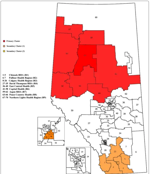
We illustrate the log-Weibull SSS on population based administrative data (age ≥ 35) for patients discharged from the emergency department (ED) who presented with atrial fibrillation and flutter (AFF) in the province of Alberta during April 1, 2010, to March 31, 2011. In 2003, the province of Alberta was divided into nine adminis-trative health areas also called Regional Health Authori-ties (RHAs) [19]. These RHA’s were further partitioned into 70 sub-Regional Health Authorities (sRHAs) (Fig. 1, numbered 1–70). The sRHAs have diverse population sizes ranging from 550 to 140,211 with a median popula-tion size of 46,075 in 2011 and are the smallest geograph-ical units available for analysis. For each sRHA’s centroid based on population, the latitude and longitude of the centroids are provided by Alberta Health [19]. Distances between the pairs of sRHA population-based centroids are ordered and used to create the nearest neighbours.

The key outcome of interest is the time from ED dis-charge for AFF to the 1st specialist visit during 365 days of the study period. The specialist in this study is con-sidered as a cardiology (CARD) or internal medicine (INMD). A specialist follow-up visit can occur between ED end time, to the end of the study. Each discharged ED presentation during April 1, 2010, to March 31, 2011, with a follow-up visit to the specialist during its ED end time, to March 31, 2011 is considered a complete time to event outcome. If the patient did not have specialist visit by the end of the study (March 31, 2011), the outcome is referred to as right (type-I) censored. Each Alberta resident making at least one discharged ED presenta-tion for AFF during the fiscal year is referred to as a case (patient).

(5)

median time to event for the whole dataset is 81 days and the corresponding 95% confidence interval (CI) is 76–86 days.

(6)

RHAs. This cluster is identified with 260 observed num-ber of cases. The LLR is 710.75 with the associated p

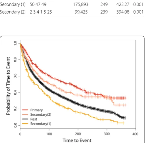
value (P) of 0.001. This SSS provides two different statisti-cally significant secondary clusters. The first one is a part of R6 and the second cluster is a combination of sRHAs from R1 and R3. Median times to event are 177, 51, and 104 days for inside the primary, secondary (1), and sec-ondary (2) detected clusters, respectively. The corre-sponding 95% CI’s are 128–223, 38–75, and 77–150 days. For the entire province, collectively excluding the pri-mary and both secondary clusters, the median event time is 78 days and the 95% CI is (71, 84) days. Figure 2 shows the Kaplan–Meier curves for the detected pri-mary and secondary clusters and the rest of the province. The SSS based on the Weibull distribution has also been applied to the same Alberta Health data, and is capable of detecting the same primary cluster as of the log-Weibull distribution i.e., from R7-R9 RHA’s, with no significant secondary cluster.

Simulation studies

Simulation studies are conducted to investigate the power of detecting a potential cluster and the effect of

right differential censoring on cluster detection. All of the datasets are analyzed with the log-Weibull and Weibull SSS’s. Time to event data are randomly generated for 500 individuals with five different probability models: the exponential, Weibull, Normal, gamma, and log-Weibull. The Alberta geography is used as the geography for analysis and the Alberta population is used to create the zones for the simulation studies. Like the spatial scan analysis of the real administrative data, an upper bound of 10% is imposed on the population size.

For all simulated datasets, a true cluster of 25 indi-viduals is created at a subregion of R201 sRHA, to have longer time to events than the rest of the province. This subregion was chosen because it was rural and away from the detected rural cluster in the real Alberta ED data. R201 was assigned the same percentage of individuals as of the real dataset (i.e., approximately 5% cases in each simulated data). This choice was feasible for simulation studies to run in a reasonable amount of time. Right dif-ferential censoring is added with the ratios of 20%:20%, 20%:40%, and 40%:20% for inside:outside the true cluster. For example, 20%:40% means that 20% censoring is used within the true cluster and 40% outside the true cluster.

One thousand simulated datasets are generated from the probability models defined above using the differen-tial censoring settings under the alternative hypotheses of the existence of longer than expected time to event clus-ters. The choice of 1000 simulations is the same as what was chosen for the development of the Weibull SSS [10] and was computationally timely. For symmetry, param-eters for each probability model are chosen in such a way that they provide a constant mean of 2 outside the true cluster and means of 10, 15, and 20 inside the true cluster for each censoring ratio. These values were chosen to be similar to the inside:outside times to event means ratio from real data used in the application.

For each simulated dataset, 999 random permutations are performed to get the p values from the permutation testing procedure. Let, Z∗,Z(m), and M represent the true cluster, the cluster identified in the mth simulations, and total number of simulations, respectively. Power is calculated as the proportion of datasets out of 1000 hav-ing p values < 0.05 [9, 10], not necessarily detecting the true cluster i.e.,

In order to observe the strength of identification of the true cluster by each SSS, three different proportions are calculated for mutually exclusive situations from 1000 randomly generated datasets under each probability

Power= 1

M

m=1

I_[_Z(m)_;P(Z(m)₎_<0.05_]. Table 1 Spatial scan results for the log-Weibull

distribution

Cluster sRHA Population Cases LLR P

Primary 64 65 68 63 60 67

66 61 124,094 260 710.75 0.001 Secondary (1) 50 47 49 175,893 249 423.27 0.001 Secondary (2) 2 3 4 1 5 25 99,425 239 394.08 0.001

(7)

model for all censoring situations. These indicators are essentially the same as those reported for the exponen-tial and Weibull based SSS’s [9, 10], and we have adapted slightly to reflect the aggregate nature of the data.

These are the proportion of datasets:

1. Perfectly identifying the true cluster PI= _M1 M

m=1

I_[_Z∗₌_Z(m)_]

;

2. Identifying a large cluster including the true cluster LC= _M1 M

m=1

I_[_Z∗_⊂_Z(m)_]

; and,

3. Not identifying the true cluster

NI= _M1 M

m=1

I_[_Z∗_Z(m)_]

.

In addition to the three cluster performance measures listed above, a global indicator for performance assess-ment has been used [22] based on the coefficient devel-oped by Tanimoto [23, 24]. The Tanimoto coefficient (TC) is computed for each simulated data set and meas-ures the similarity between a simulated and detected cluster by using the ratio of the intersecting cluster cohort to the union cluster cohort. In order to calculate TC, four types of spatial units (SUs) are calculated and defined as:

True Positive (TP) = SUs both within Z∗ and Z(m);

False Positive (FP) = SUs only within Z(m);

False Negative (FN) = SUs only within Z∗ ; and,

True Negative (TN) = SUs not within either cluster.

The TC computed for each simulated data set is

TC= _TP+FP+FNTP . The geographical region used in this

simulation study is divided into 70 SUs. When no signifi-cant cluster is detected i.e., p value is higher than 0.05, we get TP = 0, FP = 0, TN = 69, and FN = 1.

The average Tanimoto coefficient (TCa) and the cumu-lated Tanimoto coefficient (TCc) were used as the statis-tics of TC. These are defined as

TCa= _M1

M

m=1

TPm

(TPm+FPm+FNm) and

TCc=

M m=1

TPm

M m=1

(TPm+FPm+FNm)

. Global performance is

assessed using TCa and TCc by taking both location accu-racy and power into account at the same time. Guttmann et al. have assessed the superiority of TCc over TCa based on their functional properties and variability, and observed that TCc has more power of capturing low accuracy in cluster location [22].

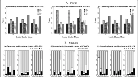
Using the log-Weibull SSS (Table 2, Figs. 3 and 4), the results show that the values of power vary from 0.326 to 0.721 for the 20%:20% censoring, from 0.148 to 0.941 for the 20%:40% censoring situation, and range from 0.350 to 0.737 for the 40%:20% censoring case. Overall, the maximum power is seen when the data are generated under the Weibull distribution and the minimum power is observed for the datasets distributed with the gamma and exponential probability models.

The proportions of datasets perfectly identifying the true cluster fluctuate for the log-Weibull SSS. They are between 0.000 and 0.310 for the 20%:20% case, range from 0.000 to 0.186 for the 20%:40% censoring ratio, and are between 0.000 and 0.264 for the 40%:20% censor-ing settcensor-ing, respectively. Under the large cluster iden-tification cohort for the log-Weibull distribution, there are high proportions of the true cluster detected. These proportions range from 0.000 to 1.000 for all three dif-ferential censoring situations. Overall, the maximum proportion of perfect identification is achieved for the datasets generated from the log-Weibull distribution. The datasets from the exponential distribution have the highest proportions of large cluster identification includ-ing the true cluster among all five probability models. A few decreases are found in the power and the strength of identification of the true cluster for each model, when comparing the 20%:20% to the 20%:40% and 40%:20% censoring cases.

For the log-Weibull SSS, the values of TCa range from 0.060 to 0.448 for all three censoring situations. The TCc values lie between 0.189 and 0.491 with very less variabil-ity among the five probabilvariabil-ity models used to generate the data.

For the Weibull SSS (Table 3, Figs. 5 and 6), the over-all results for the power and over-all the proportions’ perfor-mances of the datasets are less variable than the results of the log-Weibull SSS. The power values of detecting a potential cluster are between 0.256 and 0.971 for the 20%:20% censoring setting, range from 0.230 to 0.999 for the 20%:40% censoring ratio, and are between 0.355 and 0.981 for the 40%:20% case. The proportions of perfectly detecting a true cluster are high for all three censoring situations across all of the datasets as compared to the log-Weibull distribution, being least for the exponential model. The non-zero proportions of datasets generated under five probability distributions who do not identify the true cluster are between 0.000 and 0.997. The power values increase as the difference between the means of inside and outside the cluster increase and similar effects are seen for the strength of detection of the true cluster.

(8)

Table 2 Simulation study results for the log-Weibull spatial scan statistic

Five probability models each with three different means inside true cluster are used under three right censoring cases: a= 20%:20%, b= 20%:40%, c= 40%:20% outside cluster: mean = 2; variance = 4(Exponential), 0.188(Weibull), 2(log-Normal), 1(Gamma), and 5(log-Weibull). IC inside cluster, M mean, V variance, PI perfect Identification, LC large cluster identification, TCa average Tanimoto coefficient, TCc cumulated Tanimoto coefficient

Data distribution IC Power PI LC TCa TCc

M V a b c a b c a b c a b c a b c

Exponential 10 100.0 0.388 0.148 0.350 0.042 0.001 0.000 0.958 0.999 0.714 0.155 0.060 0.153 0.304 0.189 0.386 15 225.0 0.395 0.383 0.381 0.000 0.003 0.000 1.000 0.997 1.000 0.158 0.160 0.156 0.307 0.308 0.308 20 400.0 0.403 0.609 0.385 0.002 0.000 0.002 0.998 1.000 0.998 0.166 0.248 0.157 0.312 0.356 0.306 Weibull 10 4.0 0.554 0.913 0.522 0.310 0.128 0.127 0.014 0.041 0.127 0.252 0.435 0.248 0.444 0.489 0.452 15 10.0 0.554 0.934 0.513 0.069 0.124 0.158 0.049 0.045 0.030 0.270 0.445 0.247 0.461 0.490 0.455 20 7.0 0.559 0.941 0.573 0.122 0.148 0.020 0.039 0.001 0.089 0.274 0.448 0.283 0.462 0.491 0.468 Log-Normal 10 4.0 0.471 0.364 0.408 0.099 0.005 0.024 0.272 0.064 0.052 0.225 0.185 0.204 0.426 0.442 0.449 15 10.0 0.397 0.398 0.404 0.046 0.017 0.051 0.026 0.034 0.026 0.203 0.205 0.202 0.449 0.451 0.448 20 17.0 0.373 0.452 0.391 0.022 0.025 0.049 0.015 0.066 0.000 0.189 0.231 0.196 0.445 0.458 0.447 Gamma 10 5.0 0.400 0.425 0.432 0.005 0.025 0.050 0.027 0.134 0.021 0.207 0.216 0.217 0.446 0.453 0.448 15 7.5 0.349 0.486 0.378 0.019 0.051 0.138 0.071 0.243 0.000 0.176 0.244 0.186 0.429 0.459 0.431 20 10.0 0.326 0.525 0.380 0.025 0.076 0.118 0.118 0.326 0.035 0.163 0.253 0.186 0.416 0.454 0.430 Log-Weibull 10 5.5 0.641 0.357 0.682 0.199 0.123 0.238 0.029 0.490 0.714 0.299 0.160 0.286 0.460 0.397 0.429 15 6.0 0.721 0.344 0.705 0.103 0.186 0.209 0.062 0.760 0.744 0.347 0.152 0.298 0.474 0.389 0.436 20 6.5 0.670 0.323 0.737 0.138 0.186 0.264 0.518 0.762 0.688 0.302 0.141 0.307 0.446 0.384 0.434

A Power

B Strength

10 15 20

Exp Weib LN Gam LW (a) Censoring inside:outside cluster = 20%:20%

Inside Cluster Mean

Powe

r

0.

00

.2

0.

40

.6

0.

81

.0

10 15 20

Exp Weib LN Gam LWl (b) Censoring inside:outside cluster = 20%:40%

Inside Cluster Mean

Powe

r

0.

0

0.

20

.4

0.

6

0.

8

1.

0

10 15 20

Exp Weib LN Gam LW (c) Censoring inside:outside cluster = 40%:20%

Inside Cluster Mean

Powe

r

0.

00

.2

0.

4

0.

60

.8

1.

0

Exp Weib LN Gam LW Inside Cluster Mean=10

0.

0

0.

2

0.

4

0.

60

.8

1.

0

0.

00

.2

0.

40

.6

0.

81

.0

Exp Weib LN Gam LW

NI LC PI

Inside Cluster Mean=20

0.

00

.2

0.

40

.6

0.

81

.0

(a) Censoring inside:outside cluster = 20%:20%

0.

00

.2

0.

40

.6

0.

81

.0

0.

00

.2

0.

40

.6

0.

81

.0

Exp Weib LN Gam LW NI LC PI

0.

0

0.

2

0.

40

.6

0.

81

.0

(b) Censoring inside:outside cluster = 20%:40%

0.

0

0.

2

0.

40

.6

0.

8

1.

0

0.

00

.2

0.

40

.6

0.

8

1.

0

0.

00

.2

0.

40

.6

0.

81

.0

(c) Censoring inside:outside cluster = 40%:20%

Fig. 3 Power and strength of the log-Weibull spatial scan statistic for cluster detection under right differential censoring. Datasets are generated using five probability models with outside cluster mean = 2. PI perfect identification, LC large cluster (including true cluster), NI no identification,

(9)

results for the spatial cluster detection based on power, proportions of cluster detection and global detection test regardless of the probability model used for the data

generation, whereas the performance of the log-Weibull SSS is best when the datasets are generated from the log-Weibull distribution.

A Average Tanimoto Coefficient

B Cumulated Tanimoto Coefficient

10 15 20

Inside Cluster Mean Average Tanimoto Coefficient 0.0

0.

2

0.

40

.6

0.

81

.0

10 15 20

Exp Weib LN Gam LW (b) Censoring inside:outside cluster = 20%:40%

0.

20

.4

0.

60

.8

1.

0

10 15 20

0.

20

.4

0.

60

.8

1.

0

10 15 20

Inside Cluster Mean Cumulated Tanimoto Coefficient 0.0

0.

2

0.

40

.6

0.

81

.0

10 15 20

0.

20

.4

0.

60

.8

1.

0

10 15 20

0.

20

.4

0.

60

.8

1.

0

Fig. 4 Average and cumulated Tanimoto coefficients of the log-Weibull spatial scan statistic for cluster detection under right differential censoring. Datasets are generated using five probability models with outside cluster mean = 2

Table 3 Simulation study results for the Weibull spatial scan statistic

Five probability models each with three different means inside true cluster are used under three right censoring cases: a= 20%:20%, b= 20%:40%, c= 40%:20% outside cluster: mean = 2; variance = 4(Exponential), 0.188(Weibull), 2(log-Normal), 1(Gamma), and 5(log-Weibull). IC inside cluster, M mean, V variance, PI perfect identification, LC large cluster, identification TCa average Tanimoto coefficient, TCc cumulated Tanimoto coefficient

Data distribution IC Power PI LC TCa TCc

M V a b c a b c a b c a b c a b c

(10)

A Power

B Strength

10 15 20

Inside Cluster Mean

Powe r 0. 00 .2 0. 40 .6 0. 81 .0

10 15 20

Inside Cluster Mean

Powe r 0. 00 .2 0. 40 .6 0. 81 .0

10 15 20

Inside Cluster Mean

Powe r 0. 00 .2 0. 4 0. 6 0. 81 .0

0. 00 .2 0. 4 0. 6 0. 8 1. 0

0. 00 .2 0. 40 .6 0. 8 1. 0

0. 00 .2 0. 40 .6 0. 81 .0

(a) Censoring inside:outside cluster = 20%:20%

0. 00 .2 0. 40 .6 0. 81 .0

0. 0 0. 20 .4 0. 60 .8 1. 0

(b) Censoring inside:outside cluster = 20%:40%

0. 00 .2 0. 40 .6 0. 81 .0

0. 00 .2 0. 40 .6 0. 8 1. 0

0. 0 0. 20 .4 0. 60 .8 1. 0

(c) Censoring inside:outside cluster = 40%:20%

Fig. 5 Power and strength of the Weibull spatial scan statistic for cluster detection under right differential censoring. Datasets are generated using five probability models with outside cluster mean = 2. PI perfect identification, LC large cluster (including true cluster), NI no identification,

Exp exponential, Weib Weibull, LN log-normal, Gam Gamma, LW log-Weibull

A Average Tanimoto Coefficient

B Cumulated Tanimoto Coefficient

10 15 20

Inside Cluster Mean

Av erage Ta nimoto Coefficien t 0. 0 0. 2 0. 40 .6 0. 81 .0

10 15 20

Inside Cluster Mean

Av erage T animoto Coefficient 0. 00 .2 0. 4 0. 60 .8 1. 0

10 15 20

Inside Cluster Mean

Av erage T animoto Coefficient 0. 0 0. 20 .4 0. 60 .8 1. 0

10 15 20

Inside Cluster Mean

Cu mu late d Ta nimoto Coefficien t 0. 0 0. 2 0. 40 .6 0. 81 .0

10 15 20

Inside Cluster Mean

Cu mu late d Ta nimoto Coefficien t 0. 00 .2 0. 4 0. 60 .8 1. 0

10 15 20

Inside Cluster Mean

Cu mu late d Ta nimoto Coefficien t 0. 0 0. 20 .4 0. 60 .8 1. 0

(11)

Discussion

The spatial scan statistic (SSS) is a widely used statistical technique for the identification of the spatial clusters of different data types by using various probability distribu-tions. In the context of time to event data, the SSS has the ability to detect geographical clusters of cases with either longer and/or shorter than expected event times. These clusters can be adjusted for censoring, if the appropriate probability model is used.

We have proposed the SSS for the log-Weibull distri-bution as a new approach for detecting spatial clusters for time to event data. The log-Weibull distribution has wide applications in extreme value theory for modeling extreme and rare events. The new log-Weibull method and the Weibull SSS are applied to administrative data from Alberta Health consisting of time from ED dis-charge for an AFF presentation to 1st specialist visit within 365 days in Alberta during 2010–2011. Results from the SSS show that the primary cluster is detected at the Peace Country, Northern Lights, and Aspen regional Health Authorities. The most likely cluster is comprised of rural areas in northern Alberta which have sparse or low population and have further distances to major met-ropolitan centres. The results suggest that people living in these northern rural areas may not have regular or quick access to the follow-up care to a specialist after an ED presentation. Our results are in agreement with the rec-ognized issue of health care access for rural residents and strategies such as mobile services, telehealth, and rotat-ing specialists have been suggested and/or implemented [25]. While we recognize that the censoring might be quite early for the patients with an ED visit in late 2011 and the methods may be effected by short follow-up, the effects would be across all areas of the province and we feel that the results are likely linked to real clustering and are plausible given the recognized issue of health care access.

The simulation studies indicate that the power of detecting the potential cluster is higher for the 20%:20% censoring ratio as compared to the 20%:40% and 40%:20% settings. This comparison is also true in the context of identification of a true cluster. When either the Weibull or log-Weibull distributions is used for the SSS, the effect of the right differential censoring on power and detection of the true cluster is similar. For both of the probability models used under the SSS’s, as the difference between means of time to event data increase inside and outside the true cluster, the power and proportion of detection of the true cluster also increase. It can be observed from the overall results of both SSS’s that the Weibull SSS has good power for detecting a potential cluster for the data-sets distributed with any of the five probability models used in this study. However, overall the log-Weibull SSS’s

performance is satisfactory for the data distributed as the log-Weibull. For the identification of the true cluster, the Weibull SSS shows less variability on the simulated data-sets than the log-Weibull SSS. The log-Weibull SSS shows the most power to detect a true cluster for the datasets generated from the log-Weibull distribution. When vari-ous differential censoring situations are considered, the global performance indicators for the log-Weibull SSS do not vary widely. Conversely, when there was less cen-soring inside the cluster than outside the cluster, the log-Weibull SSS had highly variable performance that depended on the underlying data distribution.

The results based on the global indicator for perfor-mance assessment also support the above conclusions, identifying that the Weibull SSS detects the true clus-ter with more power and location accuracy both at the same time, whereas the log-Weibull SSS shows high sig-nificant cluster detection accuracy for the datasets gen-erated from log-Weibull probability distribution. It is also observed that the log-Weibull distribution has a good ability to detect a broader cluster including the true cluster instead of identifying exact true cluster. It is sug-gested that the log-Weibull SSS can be used to detect a spatial cluster for the time to event data distributed as log-Weibull. Based on the simulation study results for both SSSs, the log-Weibull SSS proved to be less effective than the Weibull SSS when the dataset is generated from the exponential distribution. When the underlying data distribution is not exponential, the log-Weibull SSS has slightly reduced performance than the Weibull SSS; how-ever, the log-Weibull SSS had similar performance across different underlying data distributions, especially when the censoring ratio is higher inside the true cluster than outside the true cluster.

There are many opportunities for future work. For example, the proposed methodology based on the SSS for the log-Weibull distribution does not adjust for impor-tant factors such as age and gender. In future, such covar-iates can be adjusted in the analysis of the identification of potential clusters for time to event data. Furthermore, the new developed method can only be performed on a purely spatial setting. The space–time scan statistic has been developed by other authors in both retrospective [15] and prospective [16] ways. In the future, the SSS based on the log-Weibull distribution can be extended to the space–time setting, and similar simulation stud-ies can be performed to investigate power of detection of space–time clusters.

Conclusions

(12)

compared and contrasted for time to event data gener-ated from simulations. The simulation studies suggest that the SSS based on the log-Weibull distribution per-forms well for log-Weibull data. The log-Weibull distribu-tion, being a specialized case of the generalized extreme value distribution, has a wide application in extreme value theory for modeling extreme and rare events.

Abbreviations

AFF: atrial fibrillation and flutter; CARD: cardiology; CI: confidence interval; ED: emergency department; INMD: internal medicine; LLR: log likelihood ratio; MLE’s: maximum likelihood estimators; P: p value; PDF: probability density function; RHAs: Regional Health Authorities; SSS: spatial scan statistics; sRHAs: sub-Regional Health Authorities; PI: perfect identification; LC: large cluster identification; NI: no identification; TP: true positive; FP: false positive; FN: false negative; TN: true negative; TCa: average Tanimoto coefficient; TCc: cumulated

Tanimoto coefficient.

Authors’ contributions

Both authors have contributed in the conception and design of the study, analysis, and interpretation of data. RR obtained the funding and directed the study. IU wrote the 1st draft and RR revised it critically for important intellec-tual content. Both authors read and approved the final manuscript.

Author details

University of Alberta, 11405 87 Avenue NW, Edmonton, AB T6G 1C9, Canada.

Univer-sity of Alberta, 11405 87 Avenue NW, Edmonton, AB T6G 1C9, Canada.

Acknowledgements

Authors thank Alberta Health for providing the data. Disclaimer: This study is based in part on data provided by Alberta Health. The interpretation and con-clusions contained herein are those of the researchers and do not necessarily represent the views of the Government of Alberta. Neither the Government nor Alberta Health express any opinion in relation to this study.

Competing interests

The authors declare that they have no competing interests

Availability of data and materials

Data is the property of Alberta Health and the authors are not allowed to pro-vide the data. Requests can be made for the same data from Alberta Health for researchers who meet the criteria for access to confidential data. Research-ers are welcome to inquire for further information at [email protected] or visit http://www.healt h.alber ta.ca/initi ative s/healt h-resea rch.html.

Consent for publication

Not applicable.

Ethics approval and consent to participate

The University of Alberta health research ethics board approved this study. Individual consent was not required.

Funding

This study is funded by a Discovery Grant held by Professor Rosychuk from the Natural Sciences and Engineering Council of Canada (NSERC; Ottawa, Canada). Sponsor had no role in the study design, analysis and interpretation of data, writing of the report, and in the decision to submit the article for publication.

Publisher’s Note

Springer Nature remains neutral with regard to jurisdictional claims in pub-lished maps and institutional affiliations.

Received: 16 November 2017 Accepted: 25 May 2018

References

1. Stevenson JR, Emrich CT, Mitchell JT, Cutter SL. Using building permits to monitor disaster recovery: a spatio-temporal case study of coastal Missis-sippi following Hurricane Katrina. Cartogr Geogr Inf Sci. 2010;37(1):57–68. 2. Coulston JW, Riitters KH. Geographic analysis of forest health indicators

using spatial scan statistics. Environ Manag. 2003;31:764–73.

3. Marcos RDLF, Marcos CDLF. From star complexes to the field: open cluster families. Astrophys J. 2008;672:342–51.

4. Usher BM, Allen KL. Identifying kinship clusters: SatScan for genetic spatial analysis. Am J Phys Anthropol. 2005;126(Suppl 40):210–1. 5. Margai F, Henry N. A community-based assessment of learning

dis-abilities using environmental and contextual risk factors. Soc Sci Med. 2003;56:1073–85.

6. Kulldorff M, Nagarwalla N. Spatial disease clusters-detection and infer-ence. Stat Med. 1995;14:799–810.

7. Costa MA, Assunção RM. A fair comparison between the spatial scan and the Besag–Newell disease clustering tests. Environ Ecol Stat. 2005;12:301–19.

8. Kulldorff M. A spatial scan statistic. Commun Stat-Theory Methods. 1997;26:1481–96.

9. Huang L, Kulldorff M, Gregorio D. A spatial scan statistic for survival data. Biometrics. 2007;63:109–18.

10. Bhatt V, Tiwari N. A spatial scan statistic for the survival data based on Weibull distribution. Stat Med. 2013;33:1867–76.

11. Jung I, Kulldorff M, Klassen A. A spatial scan statistic for ordinal data. Stat Med. 2007;26:1594–607.

12. Jung I, Kulldorff M, Richard OJ. A spatial scan statistic for multinomial data. Stat Med. 2010;29:1910–8.

13. Kulldorff M, Huang L, Konty K. A scan statistic for continuous data based on the normal probability model. Int J Health Geogr. 2009;8:58. 14. Rosychuk RJ, Chang H-M. A spatial scan statistic for compound Poisson

data. Stat Med. 2013;32:5106–18.

15. Kulldorff M, Athas W, Feuer E, Miller B, Key C. Evaluating cluster alarms: a space–time scan statistic and brain cancer in Los Alamos. Am J Public Health. 1998;88:1377–80.

16. Kulldorff M. Prospective time periodic geographical disease surveillance using a scan statistic. J R Stat Soc. 2001;A164:61–72.

17. Reliablity HotWire: The emagazine for the reliability professional. 2005.

http://www.weibu ll.com/hotwi re/issue 56/relba sics5 6.htm. Accessed 16 Sept 2015.

18. Knijnenburg TA, Wessels LFA, Reinders MJT, Shmulevich I. Fewer permuta-tions, more accurate p values. Bioinformatics. 2009;25:i161–8.

19. Ellehoj E, Schopflocher D. Calculating small areas analysis: Definition of sub-regional geographic units in Alberta. Edmonton: Alberta Health and Wellness; 2003.

20. R Core Team. R: A language and environment for statistical computing. R Foundation for Statistical Computing, Vienna, Austria, 2014. http://www. Rproj ect.org/.

21. TIBCO Software Inc. S-PLUS 8 Version 8.1.1. 2008.

22. Guttmann A, Li X, Feschet F, Gaudart J, Demongeot J, Boire J, Ouchchane L. Cluster detection tests in spatial epidemiology: a global indicator for performance assessment. PLoS ONE. 2015;10(6):e0130594.

23. Tanimoto TT. IBM internal report. IBM: Technical Report; 1957. 24. Rogers DJ, Tanimoto TT. A computer program for classifying plants.

Sci-ence. 1960;132:1115–8.