Creating a Consistent Oceanic Multi-decadal Intercalibrated TMI-GMI Constellation Data Record

(1)

University of Central Florida University of Central Florida

STARS

Electronic Theses and Dissertations, 2004-2019

2018

Creating a Consistent Oceanic Multi-decadal Intercalibrated

TMI-GMI Constellation Data Record

GMI Constellation Data Record

Ruiyao Chen

University of Central Florida

Part of the Electrical and Computer Engineering Commons

Find similar works at: https://stars.library.ucf.edu/etd

University of Central Florida Libraries http://library.ucf.edu

This Doctoral Dissertation (Open Access) is brought to you for free and open access by STARS. It has been accepted for inclusion in Electronic Theses and Dissertations, 2004-2019 by an authorized administrator of STARS. For more information, please contact [email protected].

STARS Citation STARS Citation

Chen, Ruiyao, "Creating a Consistent Oceanic Multi-decadal Intercalibrated TMI-GMI Constellation Data Record" (2018). Electronic Theses and Dissertations, 2004-2019. 5816.

(2)

CREATING A CONSISTENT OCEANIC MULTI-DECADAL

INTERCALIBRATED TMI-GMI CONSTELLATION DATA RECORD

by

RUIYAO CHEN

B.S. Electrical Engineering, Wuhan University of Science and Technology, 2012 M.S. Electrical Engineering, University of Central Florida, 2014

A dissertation submitted in partial fulfillment of the requirements for the degree of Doctor of Philosophy

in the Department of Electrical Engineering and Computer Science in the College of Engineering and Computer Science

at the University of Central Florida Orlando, Florida

Spring Term 2018

(3)

ii

(4)

iii

ABSTRACT

The Tropical Rainfall Measuring Mission (TRMM), launched in late November 1997 into a low earth orbit, produced the longest microwave radiometric data time series of 17-plus years from the TRMM Microwave Imager (TMI). The Global Precipitation Measuring (GPM) mission is the follow-on to TRMM, designed to provide data continuity and advance precipitation measurement capabilities. The GPM Microwave Imager (GMI) performs as a brightness temperature (Tb) calibration standard for the intersatellite radiometric calibration (XCAL) for the other constellation members; and before GPM was launched, TMI was the XCAL standard. This dissertation aims at creating a consistent oceanic multi-decadal Tb data record that ensures an undeviating long-term precipitation record covering TRMM-GPM eras. As TMI and GMI share only a 13-month common operational period, the U.S. Naval Research Laboratory’s WindSat radiometer, launched in 2003 and continuing today provides the calibration bridge between the two. TMI/WindSat XCAL for their >9 years’ period, and WindSat/GMI XCAL for one year are performed using a robust technique developed by the Central Florida Remote Sensing Lab, named CFRSL XCAL Algorithm, to estimate the Tb bias of one relative to the other. The 3-way XCAL of GMI/TMI/WindSat for their joint overlap period is performed using an extended CFRSL XCAL algorithm. Thus, a multi-decadal oceanic Tb dataset is created. Moreover, an important feature of this dataset is a quantitative estimate of the Tb uncertainty derived from a generic Uncertainty Quantification Model (UQM). In the UQM, various sources contributing to the Tb bias are identified systematically. Next, methods for quantifying uncertainties from these sources are developed and applied individually. Finally, the resulting independent uncertainties are combined into a single overall uncertainty to be associated with the Tb bias on a channel basis. This

(5)

iv

dissertation work is remarkably important because it provides the science community with a consistent oceanic multi-decadal Tb data record, and also allows the science community to better understand the uncertainty in precipitation products based upon the Tb uncertainties provided.

(6)

v

To Mom & Dad for your love, strength, effort, hard work that drive me to this far. You are the biggest inspiration in my entire life.

To my brother Peng, you are special and wonderful in my heart

To my husband Bing for making me laugh, wiping my tears, hugging me tight, and keeping me strong. You are my everything.

(7)

vi

ACKNOWLEDGMENTS

I would like to express my sincere gratefulness and appreciation to my advisor, Dr. W. Linwood Jones, for his guidance, dedication, patience, and support over the years. Your mentorship has propelled me into the professional I am in and has pushed me beyond my goals.

I would like to thank my committee members: Dr. Wasfy Mikhael, Dr. Lei Wei, Dr. Thomas Wilheit and Dr. Darren McKague for their ideas, discussions and comments that have been absolutely invaluable for this dissertation.

I would like to acknowledge Dr. Daoji Li for sharing his statistical expertise during this process. I would like to thank Dr. David Draper for his response to my technical questions regarding satellite instruments. I would like to thank the NASA GPM XCAL Working Group for creating the space for knowledge sharing and discussions.

I would like to thank all my colleagues and friends in CFRSL for their unflinching support and encouragement, and for bringing out the potential in me. I really appreciate all the good times we shared together in the workplace. You are all the best.

I would like to acknowledge the NASA Precipitation Processing System for providing satellite data for this dissertation work. The financial support to pursue my Ph.D. degree was sponsored by NASA grants.

(8)

vii

LIST OF FIGURES

Figure 1-1 Desired Observing Characteristics for Weather and Climate Applications (*Courtesy

of Graeme Stevens). ... 3

Figure 2-1 The TRMM observatory with the TMI instrument circled in red. ... 5

Figure 2-2 The GPM observatory with the GMI instrument circled in red. ... 6

Figure 2-3 The WindSat radiometer on board the Coriolis satellite. ... 8

Figure 3-1 Block diagram of the normalization process in CFRSL XCAL Algorithm. ... 10

Figure 3-2 Radiative Transfer Equivalent Block Diagram. ... 12

Figure 3-3 Block diagram of XCAL double difference technique. ... 13

Figure 3-4 Periods of collocated datasets. ... 17

Figure 3-5 DD from GMI & TMI inter-calibration stratified by latitude, blue line represents DD calculated using RSS RTM, and red line is XCAL RTM. ... 18

Figure 3-6 DD anomaly for GMI & SSMIS-F17 with yaw = 0°/180° and asc/des orbits. Blue color represents that using RSS RTM, and red color is XCAL RTM... 19

Figure 3-7 Triple difference between the DD values from GMI and TMI for XCAL and RSS RTM’s by channel... 20

Figure 4-1 Monthly average TMI-WindSat double difference bias time-series at 10 V-, 10 H, 37 V- and 37 H-pol channels, for XCAL year and 2011. ... 26

Figure 4-2 Monthly average TMI-WindSat double difference bias of ascending passes at all channels, for XCAL year and 2011. ... 26

Figure 4-3 Monthly average TMI-WindSat double difference of asc.(top) & dsc. (bottom) passes, through north hemisphere, at 10 V, for XCAL year and 2011. ... 27

(12)

xi

Figure 4-4 Example of near-simultaneous orbits (May 21, 2014) from GMI, TMI and WindSat on a global map (upper panel), with 3-way collocated 1°×1° boxes within ±2-hour shown in the expanded image (lower panel). ... 30 Figure 4-5 Distribution of 3-way collocations for GMI, TMI and WindSat over oceans, within ±2-hour time-window for the over-lap period of March 2014-March 2015. Upper left-hand panel presents the collocations, and the color scale represents the number. The upper right-hand panel represents TMI/WindSat DD biases, the lower panels are the WindSat/GMI and the TMI/GMI DD biases (left to right), and the color bar on the right side of each panel indicates the value of bias. ... 31 Figure 4-6 Monthly DD of 3-way inter-calibration among GMI, TMI and WindSat by radiometer channel. ... 33 Figure 4-7 Zonal stratification of radiometer channel DD’s for the overlap period. ... 34 Figure 4-8 Radiometer channel bias anomalies (DD – mean-DD) stratified by the average scene Tbobsfor the reference radiometer, which is WindSat for TMI &WindSat, and GMI for the other two radiometer comparisons. ... 35 Figure 4-9 Radiometer channel bias anomalies (DD – mean-DD) stratified by GDAS ocean surface wind speed for the overlap period. ... 36 Figure 5-1 Diagram of Uncertainty Quantification Model. ... 39 Figure 5-2 Sources that contribute to the calibration bias uncertainty. ... 42 Figure 5-3 Double difference mean and STD of the common 9 channels between TMI and GMI for the 8 cases using different temporal resolutions. The dots represent mean values, and bars crossing the dots represent the values. ... 46

(13)

xii

Figure 5-4 Block diagram of RTM. ... 49 Figure 5-5 Select 8 regions that cover the whole oceans. ... 51 Figure 5-6 An example of randomly sampled sea surface temperature histograms at region 1. .. 52 Figure 5-7 An example of double difference histograms for each channel at Region 1. ... 54 Figure 5-8 Uncertainty Estimates of 10,400 iterations grouped in region for each channel using Mono absorption model. ... 55 Figure 5-9 Uncertainty Estimates of 10,400iterations grouped in region for each channel using Rosenkranz absorption model. ... 55 Figure 5-10 Uncertainty Estimates of 10,400 iterations grouped in channel for each region using Mono absorption model. ... 56 Figure 5-11 Uncertainty Estimates of 10,400 iterations grouped in channel for each region using Rosenkranz absorption model. ... 57 Figure 5-12 Regional standard uncertainty along with the total standard uncertainty for each channel. ... 59 Figure 5-13 Difference (∆Tb) of the Planck brightness temperature from Rayleigh-Jeans Tb at Tb varying between 0 and 300 K. ... 62 Figure 5-14 Difference (∆Tb) of the Planck brightness temperature and Rayleigh-Jeans Tb at frequency varying between 0 and 300 GHz. ... 62 Figure 5-15 Difference (∆DD) of ∆Tbbetween TMI and GMI of their 9 common channels. .. 63 Figure 5-16 Standard uncertainty as a function of absolute difference between GMI and TMI frequencies. ... 64

(14)

xiii

Figure 5-17 Diagram of uncertainty estimation procedure for Mono and Rosenkranz model deviation. ... 65 Figure 5-18 Diagram of uncertainty estimation procedure for RSS and Elsaesser model deviation. ... 65 Figure 5-19 Diagram of uncertainty estimation procedure for GDAS and ERA-I model deviation. ... 66 Figure 6-1 Mean and standard deviation of calibration bias of TMI relative to WindSat for 6 years between 2005 and 2014. ... 70 Figure 6-2 Monthly calibration bias of TMI relative to WindSat for 6 years between 2005 and 2014... 72 Figure 6-3 Mean, standard deviation and spatial uncertainty of double difference bias between TMI and WindSat per channel for year 2011. ... 73 Figure 6-4 Mean, standard deviation and temporal uncertainty of double difference bias between TMI and WindSat per channel for year 2011. ... 73 Figure 6-5 Spatial uncertainties of double difference biases between TMI and WindSat per channel for 6 different years. ... 74 Figure 6-6 Temporal uncertainties of double difference biases between TMI and WindSat per channel for 6 different years. ... 74 Figure 6-7 Uncertainty Estimates of 18,400 iterations grouped in region for each channel for TMI and WindSat intercalibration of year 2011. ... 76 Figure 6-8 Uncertainty Estimates of 18,400 iterations propagated from GDAS are grouped in channel for each region for TMI and WindSat intercalibration of year 2011. ... 76

(15)

xiv

Figure 6-9 Uncertainty Estimates from GDAS of TMI and WindSat intercalibration for the 6 years.

... 77

Figure 6-10 Uncertainty Estimates of TMI and WindSat intercalibration in Rayleigh-Jeans Approximation from Planck’s Law for the 6 years. ... 77

Figure 6-11 Uncertainty Estimates in MONO and Rosenkranz atmosphere absorption models for TMI and WindSat intercalibration for the 6 years. ... 78

Figure 6-12 Uncertainty Estimates in Elsaesser and RSS surface emissivity models for TMI and WindSat intercalibration for the 6 years. ... 78

Figure 6-13 Uncertainty Estimates in discrepancy between ERA-I and GDAS models for TMI and WindSat intercalibration for the 6 years. ... 79

Figure 6-14 Spatial uncertainty of WindSat/GMI intercalibration. ... 80

Figure 6-15 Temporal uncertainty of WindSat/GMI intercalibration. ... 81

Figure 6-16 GDAS uncertainty of WindSat/GMI intercalibration grouped in region. ... 82

Figure 6-17 GDAS uncertainty of WindSat/GMI intercalibration grouped in channel... 82

Figure 6-18 Rayleigh-Jeans uncertainty of WindSat/GMI intercalibration. ... 83

Figure 8-1 Latitude dependence of calibration bias of TMI relative to WindSat. The patterns are stable along the years, and the water vapor channels (19V, 19H, and 22V) present smile shape and a peak—to-peak 0.5 drift along the whole latitude range. ... 95

Figure 8-2 Monthly DD anomaly in time series from 2005 to 2014, where a cyclic pattern is shown. ... 96

Figure 8-3 Observed mean single difference and simulated (modeled) mean single difference of TMI relative to WindSat for the 6 years. ... 96

(16)

xv

Figure 8-4 Observed and simulated Tb anomaly of TMI for the 6 years. ... 97

Figure 8-5 Observed and simulated Tb anomaly of WindSat for the 6 years. ... 97

Figure 8-6 TMI single differences for the 6 years. ... 98

Figure 8-7 WindSat single differences for the 6 years. ... 98

Figure 8-8 Averaged DD anomaly for each quarter (3 months) of TMI relative to GMI for the 6 years. ... 99

(17)

xvi

LIST OF TABLES

Table 2-1: GMI, TMI, and WindSat instrument parameters (source: [2], [5], [6]). ... 7

Table 3-1 DD values between TMI and GMI with different atmosphere absorption models. ... 15

Table 3-2 Imager channels in GMI constellation. ... 16

Table 3-3 Mean and std of double differences... 21

Table 4-1 DD mean and std between TMI and WindSat for V-pol. ... 24

Table 4-2 DD mean and std between TMI and WindSat for H-pol. ... 25

Table 4-3 Double differences mean/std, upper panel is ±1 hr and lower panel is ±2 hr temporal resolution... 32

Table 5-1 Temporal resolutions. ... 44

Table 5-2 Spatial resolutions. ... 45

Table 5-3 Standard uncertainty in sampling process. ... 47

Table 5-4 Uncertainty in GDAS geophysical parameters for 8 oceanic regions [25]. ... 53

Table 5-5 Double difference bias between TMI and GMI. ... 58

Table 5-6 Standard uncertainties propagated from geophysical parameters. ... 58

Table 5-7 Regional standard uncertainties propagated from geophysical parameters. ... 59

Table 5-8 Standard uncertainty propagated from Rayleigh-Jeans approximation... 64

Table 5-9 Standard uncertainty for Mono and Rosenkranz model deviation. ... 66

Table 5-10 Standard uncertainty for RSS and Elsaesser model deviation... 66

Table 5-11 Standard uncertainty for GDAS and ERA-I deviation. ... 67

Table 5-12 rss uncertainty without GMI calibration uncertainty... 68

(18)

xvii

Table 6-1 Averaged calibration biases of TMI/ WindSat intercalibration. ... 70

Table 6-2 Combined standard uncertainty of TMI/ WindSat intercalibration. ... 79

Table 6-3 Uncertainty from model deviation... 83

(19)

1

1 INTRODUCTION

1.1 Significance of Radiometric Intercalibration

With an international network of multiple satellites carrying microwave radiometers with similar designs, it is possible to provide a near-real time global observations of earth radiance and to further ensure unified estimates of precipitation. Because these microwave radiometers are built and launched by different space agencies with widely varying specifications and capabilities, it is necessary that the brightness temperatures (Tb), which are the inputs to the precipitation retrieval process, be physically consistent between sensors. This means that differences in the observed Tb between sensors should agree with the expected differences based on radiative transfer model simulations that account for variations in the observing frequencies, channel bandwidths, view angles, etc. Properly accounting for sensor differences is critical to producing consistent precipitation estimates between radiometers, and this is the only way to ensure that observed changes in precipitation are real and not the result of sensor calibration issues.

1.2 History of GPM XCAL Group

The GPM Intersatellite Calibration Working (XCAL) Group was established in 2007 as an ad hoc working group within the NASA Precipitation Measurement Missions (PMM) science team. The XCAL group has responsibility for the intercalibrated level 1C Tb files that are used as input for the radiometer retrieval algorithm. Prior to the launch of GPM this involved developing the level 1C format and producing initial calibration tables for the constellation sensors using TMI as the reference standard. After the launch of the GPM Core Observatory, the XCAL group initially

(20)

2

focused on the GMI on-orbit radiometric calibration to ensure it provided the best possible calibration reference for the other microwave radiometers in the GPM constellation. Once the GMI calibration was finalized for the version 4 (V04) reprocessing, the group worked to identify issues affecting the calibration and stability of the constellation radiometers, developed corrections for these issues, and then produced intercalibration tables to adjust for residual sensor calibration differences in a physically consistent manner. XCAL has also served as a general-purpose consultant to the rest of the science team on radiometer technical issues [1]. The XCAL group currently consisted of four teams, namely: University of Maryland (formerly Texas A&M University, Colorado State University, University of Michigan, and the Central Florida Remote Sensing Lab (CFRSL) at the University of Central Florida.

1.3 Dissertation Objectives

Despite the difficulty in forecasting climate change and its consequences, it is imperative to address the wide uncertainties and long-term stabilities in our understanding of climate change and its effects (shown in Figure 1-1). Therefore, systematic analysis and consistent methods of incorporating uncertainty into global change assessments will become increasingly necessary. Therefore, this dissertation aims at creating a consistent, multi-decadal, intercalibrated, oceanic brightness temperature data record for TRMM-GPM eras using the WindSat as a radiometric calibration bridge for the 11-year time gap, with the focuses (1) to use WindSat to provide additional intercalibration for both TMI and GMI and (2) to develop a generic uncertainty quantification model which provides the uncertainty estimates associated with calibration bias.

(21)

3

Figure 1-1 Desired Observing Characteristics for Weather and Climate Applications (*Courtesy of Graeme

Stevens).

1.4 Dissertation Overview

This dissertation is aimed at creating a consistent multi-decadal oceanic brightness temperature data record for the TRMM and GPM eras. It will start with the description of TMI, GMI and WindSat instruments in Chapter 2. Chapter 3 will present the procedures involved in the CFRSL XCAL algorithm in detail. In Chapter 4, the three-way radiometric intercalibration between TMI, GMI and WindSat is shown. A generic uncertainty quantification model (UQM) is described with results analyzed in Chapter 5. It is followed with the developed UQM being applied to TMI/WindSat XCAL and WindSat/GMI XCAL, and results are presented in Chapter 6. Finally, the conclusions and future work are presented in Chapter 7 and Chapter 8 respectively.

detecting

change

understanding

processes

understanding

change

stability

unc

er

ta

int

y

low

(22)

4

2 INSTRUMENTS

2.1 TMI

The Tropical Rainfall Measuring Mission (TRMM) satellite (shown in Figure 2-1), a collaboration between NASA and the Japan Aerospace Exploration Agency (JAXA) that was launched into an earth orbit of 350 km (later boosted to 405 km) altitude and 35° inclination in late November 1997. This original 3-year science mission using a precipitation radar (PR) and a multi-frequency microwave radiometer (TRMM Microwave Imager, TMI) to measure the rainfall statistics in the tropics [2].

TMI was a conical scanning radiometer designed to provide rainfall measurements over a swath of 878 km. This multi-frequency, externally calibrated, total power radiometer design was a derivative of the Special Sensor Microwave/Imager (SSM/I), which has successfully operated on the Defense Meteorological Support Program (United States Air Force weather satellites) since 1987. After the TRMM mission was extended, its scientific role was expanded to include a constellation of cooperative international weather satellite programs that carried microwave radiometers capable of measuring rainfall, which later evolved into the current Global Precipitation Measurement (GPM) program. TMI eventually provided a 17-plus-year time-series of calibrated brightness temperature (Tb) that have remarkable value for investigating the effects of the Earth’s climate change over the tropics [3].

(23)

5

Figure 2-1 The TRMM observatory with the TMI instrument circled in red.

For the TRMM constellation, the NASA project used a single satellite radiometer rain retrieval algorithm (GPROF), which assumed all the radiometers sensors were intercalibrated. Because TRMM’s low earth orbit provided frequent near-simultaneous crossings with the polar satellites (carrying other microwave radiometers), TMI was selected as the radiometric transfer standard to perform inter-satellite radiometric cross-calibration (XCAL) of the constellation, until it was decommissioned in 2015. As a result, TRMM collected 17 years of rainfall data and created an invaluable rainfall climatology, which serves the international global hydrological cycle research community [1].

(24)

6 2.2 GMI

The follow-on Global Precipitation Measurement (GPM) mission satellite was launched in February 2014, to provide data continuity and to improve precipitation measurement capabilities. Like TRMM, the GPM observatory shown in Figure 2-2 has two primary precipitation remote sensors, namely: the Dual Frequency Precipitation Radar (DPR) and the GPM Microwave Imager (GMI). Moreover, the GPM orbit extends the coverage to over ± 65° latitude, and both sensors have improved sensitivity to measure light precipitation and snow that occurs at higher latitudes. GPM now also comprises a constellation of cooperating weather and research satellites that have suitable microwave radiometers [4].

(25)

7

GMI is also a conical scanning microwave radiometer with 13 channels of which 9 overlap with TMI, and 7 overlap with WindSat given in Table 2-1. The GMI instrument has a 1.2 m diameter antenna, which at 407 km altitude achieves higher spatial resolution than TMI and all other radiometers in the GPM constellation. Furthermore, based upon a successful 6-month on-orbit calibration/validation period, GMI’s performance has met all requirements of radiometric sensitivity and calibration stability; and as a result, it has been designated as the new radiometric transfer standard for GPM. Based on previous experience with TMI and available on-board fuel, the GPM spacecraft is estimated to operate for 10-15 years [5].

Table 2-1: GMI, TMI, and WindSat instrument parameters (source: [2], [5], [6]).

* In each channel, the left column is for GMI, the middle is for TMI and the right is for WindSat. B stands for

bandwidth and IFOV is instantaneous field of view.

2.3 WindSat

WindSat shown in Figure 2-3 is the world’s first polarimetric microwave radiometer in space, which was developed by the Naval Research Laboratory (NRL) and launched in January 2003 on board the USAF Coriolis satellite into a 840-km sun-synchronous polar orbit [6]. The

(26)

8

sensor has a conically scanning reflector antenna that produces a forward-looking swath of approximately 1000 km. It consists of 22 channels of polarized Tb; as mentioned previously, 7 channels overlap with TMI and GMI as given in Table 2-1. The WindSat radiometric calibration campaign has been believed to be an outstanding success, and excellent results have been published to provide high confidence in the Tb’s from WindSat Sensor Data Records (SDR) [6, 7].

(27)

9

3 CFRSL XCAL ALGORITHM

A robust inter-satellite calibration algorithm has been developed by CFRSL and applied to multiple microwave radiometers. It compares two satellite radiometer observations, on a channel basis, for homogeneous earth scenes, that are collocated spatially and temporally [8]. In the simplest sense, if the corresponding channels of two radiometers, with identical design, were to make an observation over the earth at the exact same time and space, the difference in their Tb’s should reflect the radiometric calibration bias between the instruments. Unfortunately, for radiometers of different designs, the situation is more complicated due to different center frequencies, bandwidths and/or earth incidence angles; thus, normalization between the radiometers is required before cross-calibration. Using the CFRSL XCAL algorithm, this normalization utilizes microwave radiative transfer theory to translate the measurement of one or the other to a common basis before comparison. This algorithm involves three procedures in the normalization process to obtain simulated Tb’s to derive the calibration biases. A block diagram of these procedures is shown in Figure 3-1.

(28)

10

Figure 3-1 Block diagram of the normalization process in CFRSL XCAL Algorithm.

3.1 Gridding Process

In this step, the raw sensor Tb’s are averaged spatially into 1°boxes, which are generated on a per orbit basis, for each sensor and each radiometer channel. For XCAL over oceans, filters are used to select clear-sky homogeneous scenes, such as standard deviation of Tb’s per box should be no more than 2 K in V-polarization (V-pol), and 3 K in H- polarization (H-pol). Because high Tb standard deviations within a box are indicative of nonhomogeneous environmental conditions, including weather fronts with rain and/or small island contamination, these boxes are removed when standard deviations exceed 2 and 3 K for vertical and horizontal polarizations, respectively. Further editing is applied at all frequencies based on the upper limits of Tb’s expected from rain-free ocean; and a conservative land mask is also applied, to filter out possible Tb contamination from nearby land pixels.

3.2 Spatial and Temporal Collocation

To assure identical environmental conditions, the two radiometers’ gridded observations along with geophysical parameters are spatially collocated within a ±1-hour time window. The primary geophysical parameters used are from the NOAA Global Data Assimilation System (GDAS) which uses the National Center for Environmental Prediction (NCEP) Global Forecast System (GFS) model (NCEP 2000 ) to provide outputs at 0000, 0600, 1200, and 1800 Greenwich Mean Time (GMT), on a 1° x 1° latitude/longitude grid [9]. These data include the vertical profiles of atmospheric temperature, pressure, humidity, and cloud water density at 21 pressure layers, as

(29)

11

well as the surface measurements of sea surface temperature, and ocean wind speed at a 10-m height. For validation purpose, a second geophysical dataset known as the European Centre for Medium-Range Weather Forecasts (ECMWF) Reanalysis Interim (ERA-I) was used, which provides the same sets of geophysical parameters but with 29 layers in the atmosphere profiles [10].

3.3 Ocean Radiative Transfer Model

When the same earth scene is observed by two radiometers of different designs, there might be significant differences in their respective brightness temperature measurements, which does not necessarily constitute calibration errors (e.g., different frequencies and incidence angles would result in different Tb’s); but with the use of a Radiative Transfer Model (RTM), it is possible to determine the expected theoretical difference in their Tb’s [11].

A block diagram of the XCAL Ocean RTM is given in Figure 3-6. This model is used to calculate the apparent brightness temperature (Tb) at the aperture of the satellite radiometer antenna, which is the desired sensor measurement. Because of an imperfect antenna and transmission losses between the antenna and receiver, the antenna temperature TA is different from the desired Tb. Nevertheless, through the application of appropriate calibration and correction algorithms, the TA may be converted into a precise estimate of Tb. The Tb at polarization p is the result of the scalar sum of three components of brightness temperature given by

𝑻𝑻𝑻𝑻(𝒔𝒔𝒔𝒔𝒔𝒔𝒔𝒔𝒔𝒔𝒔𝒔𝒔𝒔𝒔𝒔𝒔𝒔) =𝜸𝜸𝒔𝒔�𝑻𝑻𝑺𝑺𝑺𝑺𝒑𝒑 +𝑻𝑻𝒔𝒔𝒔𝒔𝒔𝒔𝒔𝒔𝒑𝒑 �+𝑻𝑻𝒖𝒖𝒑𝒑 (1) where γa is the one-way atmospheric transmissivity, TSE is the ocean surface emission, Tscat is the downwelling atmospheric emission that undergoes specular reflection, and Tup is the upwelling atmospheric temperature. Thus the RTM is a collection of subroutines that compute these

(30)

12

components, and the current NASA XCAL RTM comprises the Remote Sensing System (RSS) ocean emissivity model [12] and the Mono atmospheric absorption model [13]. Further, the RTM requires knowledge of the pertinent environmental parameters from the atmosphere and ocean surface, which are provided by numerical weather model outputs (GDAS or ERA-I).

Moreover, the XCAL group continues to evaluate and update the RTM used for intersatellite radiometric calibration; however, by agreement, each member uses the same RTM and evaluation dataset to perform their independent analysis. In this manner, the differences between radiometric biases are mostly technique related and much less dependent on RTM. Moreover, the resulting Tb differences are removed when the various satellite radiometers are normalized to the constellation radiometric standard (TMI or GMI).

(31)

13 3.4 CFRSL XCAL Algorithm

Because the environmental parameter inputs derived from numerical weather models, as well as the physics of the radiative transfer theory, are not perfect, the simulated Tb’s may have absolute Tb offsets of several Kelvin, which is not acceptable for inter-satellite calibration. To mitigate these effects Gopalan [11], developed a technique, which calculated the difference between differences (double difference) of measured and modeled (theoretical RTM) brightness temperatures. This approach was subsequently improved by Biswas et al. [8] and became the CFRSL XCAL algorithm shown in Figure 3-3. Thus using the double differences, the imperfect physics in the RTM, errors in the associated environmental parameters from GDAS, and the effects of frequency and EIA differences between radiometers, are mostly common mode and usually cancel.

Figure 3-3 Block diagram of XCAL double difference technique.

In this algorithm, there are two radiometers being cross calibrated, namely: the target radiometer (sensor to be calibrated) and the radiometric standard (reference). Within a 1° Lat/Lng box, the observed Tb’s for a particular channel are averaged to improve the noise equivalent

(32)

delta-14

Tb, NEDT, and to produce the REFobs and TGTobs. Next, the oceanic RTM (Section 3.3) is run, using the collocated environmental parameters and given sensor parameters (frequency, incidence angle and polarization), to produce theoretical simulated Tb for REFsim and TGTsim. The expected Tb single difference is defined as (TGTsim - REFsim), and the observed single difference is (TGTobs -REFobs). The final step is to calculate the double difference (DD), which is the Tb bias as:

(

_obs _obs

) (

_sim _sim

)

bias DD TGT REF TGT REF

Tb = = − − − (2)

This technique essentially cancels out any absolute bias that may exist in the RTM, and it represents the radiometric bias of the target radiometer with respect to the reference radiometer. Before retrieving precipitation, this bias will be then applied to the target radiometer Tb to be consistent with the reference radiometer (calibration transfer standard) that is usually TMI or GMI.

3.5 Ocean Radiative Transfer Model Impact on CFRLS XCAL Algorithm

The use of an oceanic RTM is an integral part of our CFRSL XCAL algorithm. Because the RTM physics is imperfect and because the geophysical parameters are likewise only estimates of their true values based on numerical weather models, it is important to assess the sensitivity of the derived Tb biases to these limitations.

3.5.1 DD Sensitivity to Atmospheric Absorption Models

Previously, the Rosenkranz models were used by the GPM XCAL Group to calculate the atmospheric absorption coefficients for: water vapor (WV) [14], cloud liquid water (CLW) [15],

(33)

15

oxygen [16], and nitrogen[17]; later the monochromatic RTM (MONO, MonoRTM) [13] replaced the Rosenkranz water vapor sub-routine in the RTM.

The DD bias between TMI and GMI are calculated using both models, and the results are presented in Table 3-1. Significant differences between these calculations occur for the channels at 23 V and the 19 V & H channels. The cause of this is suspected to be the imperfect simulation of the water vapor profiles in the numerical weather models and inadequate knowledge of the radiative transfer modeling near the 22.235 GHz water vapor line.

After considerable study within the XCAL working group, the MonoRTM was chosen to be included in the current XCAL RTM, and it was concluded that the disagreement between the two atmospheric absorption models can contribute to the uncertainty associated with the DD bias.

Table 3-1 DD values between TMI and GMI with different atmosphere absorption models.

10V 10H 19V 19H 23V 37V 37H 89V 89H

MONO DD 0.70 0.56 0.16 0.71 0.03 -0.82 1.05 0.19 -0.80

Rosenkranz DD 0.72 0.58 0.45 1.23 1.07 -0.75 1.07 0.25 -0.60

3.5.2 DD Sensitivity to Ocean Surface Emissivity Models

The contents of this section have been published in the following article:

R. Chen, H. Ebrahimi, and W. L. Jones, “Sensitivity of XCAL double difference approach to ocean surface emissivity and its impact on inter-calibration in GPM constellation,” in 2016 IEEE International Geoscience and Remote Sensing Symposium (IGARSS), 2016, pp. 871–874 [18].

(34)

16

In this section, the inter-calibration between GMI and other constellation satellite microwave radiometers is presented for 9 microwave imager channels ranging from 10 to 89 GHz (see Table 3-2), using the CFRSL XCAL algorithm with two different ocean surface emissivity models. The first RTM, known as XCAL, uses the ocean surface emissivity model by Elsaesser [19]; and the second RTM, known as Remote Sensing Systems (RSS), replaces the surface emissivity model with that of Meissner and Wentz [12]. The major difference of these models is the dependence of the surface emissivity with ocean roughness (surface wind speed). Because the majority of the imager channels’ Tb comes from the ocean surface, it is important that we assess the impact of these two models on the derived DD biases.

Table 3-2 Imager channels in GMI constellation.

GMI TMI WindSat AMSR2 SSMIS

Channel #

Central Freq & Pol

Central Freq & Pol 1 10.65 V 10.65 V 10.70 V 10.70 V - 2 10.65 H 10.65 H 10.70 H 10.70 H - 3 18.70 V 19.35 V 19.35 V 18.70 V 19.35 V 4 18.70 H 19.35 H 19.35 H 18.70 H 19.35 H 5 23.80 V 21.30 V 23.80 V 23.80 V 22.235 V 6 36.64 V 37.00 V 37.00 V 36.50 V 37.00 V 7 36.64 H 37.00 H 37.00 H 36.50 H 37.00H 8 89.00 V 85.50 V - 89.00 V 91.655 V 9 89.00 H 85.50 H - 89.00 H 91.655 H

The periods of the datasets used are shown in Figure 3-4 for different pairs of radiometers, and the corresponding results are analyzed to assess the robustness of the CFRSL XCAL algorithm to the selection of the ocean surface emissivity model.

(35)

17

Figure 3-4 Periods of collocated datasets.

The experimental data set consisted of individual 1° boxes with associated DD biases computed using two independent RTMs. The usual analysis procedure is to sort the boxes in various manners and to display the DD biases versus different parameters e.g., time, space (latitude), or environmental parameters (sea surface temperature, wind speed, integrated atmospheric water vapor and cloud liquid water). The expectation is that the true radiometric bias is a constant, independent of the sorting method.

An example of the DD biases between GMI and TMI for the two RTM’s (red = XCAL and blue = RSS) is plotted versus the box latitude in Figure 3-5. Data symbols are the mean DD’s calculated over the corresponding box latitude bins for the ~ 1-year period. Note that 10 GHz and 37 GHz results are “flat”, which indicates that the CFRSL XCAL algorithm is working well and that the results are nearly the same for both RTM’s. Results for 89 GHz are similar except there is an offset of ~ 0.2 K for the H-pol, which indicates a sensitivity to the RTM used.

(36)

18

Figure 3-5 DD from GMI & TMI inter-calibration stratified by latitude, blue line represents DD calculated

using RSS RTM, and red line is XCAL RTM.

On the other hand, DD results for 19 GHz and 23 GHz show a latitude dependence, which is most likely that the RTM does not accurately represent the theoretical Tb for water vapor that changes symmetrically about the equator. However, the V-pol results show negligible differences for the two surface emissivity models; whereas, results for 19 GHz H-pol have a significant offset of ~ 0.3 K.

When the data are sorted by ascending and descending passes for satellite yaw = 0° (flying forward) and 180° (flying backward) the DD results (Figure 3-6) exhibit no sensitivity to the two surface emissivity models. Yet, from Figure 3-5, we recognize that the DD biases for some channels are not constant. This illustrates the importance of examining the DD biases over all possible combinations of parameters to assure an accurate cross-calibration with GMI.

(37)

19

Figure 3-6 DD anomaly for GMI & SSMIS-F17 with yaw = 0°/180° and asc/des orbits. Blue color represents

that using RSS RTM, and red color is XCAL RTM.

In addition, the reason for the sensitivity of the DD biases (for certain channels) to the RTM is examined in Figure 3-7. Here the difference of the DD biases (triple difference) for the two RTM’s are plotted versus the ocean surface wind speed. Since the ocean wind speed follows a Rayleigh distribution with mean ~ 6.5 m/s, the DD result is effectively the average over wind speed between 3 – 10 m/s. Over this range, the triple difference for most channels is close to zero, except for 19 GHz H-pol, 23 GHz and 89 GHz H-pol. For these channels, differences in the emissivity model responses to wind speed cause significant changes, which are RTM dependent.

(38)

20

Figure 3-7 Triple difference between the DD values from GMI and TMI for XCAL and RSS RTM’s by channel.

Finally, the overall box average DD biases (relative to GMI) are tabulated for 7 constellation satellites, 9 channels and the two RTM’s in Table 3-3. Of the 53 combinations, the triple differences are excellent for all but 13 marked in red color, and these are associated with 19 GHz H-pol and 89 GHz H-pol discussed above.

(39)

21

Table 3-3 Mean and std of double differences.

While these models yield different Tb’s of several Kelvin, the Tb bias results are nearly identical, which shows the robustness of this XCAL technique. The anomaly presenting in 19 GHz H-pol and 89 GHz H-pol was investigated and explained by significant differences in the emissivity models for these two channels. For most of the comparisons (satellites and channels), it is apparent that the DD biases from both the XCAL and RSS RTM’s are nearly identical (< 0.1 K); indicating that the CFRSL XCAL algorithm is not sensitive to the choice of RTM. However, for the 19 GHz H-pol and 89 GHz H-pol significant differences were noted. After independent investigations of the XCAL working group, the RSS model was selected as the surface emissivity model.

(40)

22

4 THREE-WAY INTER-SATELLITE RADIOMETRIC

CALIBRATION BETWEEN GMI, TMI AND WINDSAT

The TRMM satellite launched in late November 1997 into a low earth orbit, produced the longest satellite-derived precipitation time series of 17 years. During the second half of this mission, a collection of cooperative weather satellites, with microwave radiometers, were combined to produce a 6-hour tropical precipitation product, and the TRMM Microwave Imager (TMI) was used as the radiometric transfer standard to inter-calibrate the constellation members. To continue this valuable precipitation climate data record, the Global Precipitation Mission (GPM) observatory was launched in February 2014; and the GMI became the new transfer standard that normalized the microwave radiance measurements of the GPM constellation radiometers. Because the radiometric transfer standard for this constellation has changed to GMI, it is highly desirable to perform XCAL between GMI and TMI to link the TRMM and GPM precipitation measurements to form a multi-decadal climate dataset.

Intercomparisons between TMI and the Naval Research Laboratory’s WindSat polarimetric radiometer over oceans has been conducted, from which the radiometric calibration of TMI relative to WindSat exhibited exceptional long-term radiometric stability over a period > 8 years. Results will be presented in this chapter. Moreover, for purposes of assessing global climate change, it is crucial that a seamless transfer between the TRMM and the GPM microwave Tb time series be achieved. Therefore, this chapter will also present arguments that the 3-way (WindSat, TMI and GMI) intersatellite radiometric comparisons, performed during the 13-month period overlap, can be used to bridge the TRMM and GPM eras, and assure a stable radiometric

(41)

23

calibration between the diverse constellation’s member radiometers. The instrumental parameters of the common channels of these three radiometers are listed in Table 2-1.

4.1 Long-term Radiometric Intercalibration stability of TMI and WindSat

R. Chen, A. Santos-Garcia, S. Farrar, and W. L. Jones, “Assessment of the long-term radiometric calibration stability of the TRMM microwave imager and the WindSat Satellite Radiometers,” in 2014 13th Specialist Meeting on Microwave Radiometry and Remote Sensing of the Environment (MicroRad), 2014, pp. 187–191 [20].

Since the initial XCAL meeting 11 years ago, the short-term stability of TMI has been verified by several researches, using complementary approaches [21]. This section focuses on evaluating the long-term stability of inter-satellite radiometric calibration of TMI respect to WindSat. The CFRSL XCAL algorithm described in Chapter 3 is used here to derive the radiometric calibration biases between TMI and WindSat for two one-year periods. The TMI Tb product used in this analysis was the previous version 1B11 V7; therefore, the biases are slightly different from the extended analysis over even longer time spans with the most updated TMI Tb product, 1B11 V8 [3] (will be discussed in Chapter 6), and this does not conflict with the argument that the TMI is radiometrically stable in long-term with respect to WindSat.

The assumption is that the radiometers are stable, thus, the biases should be independent of time. This is verified by comparing monthly collocations over the two one-year periods (XCAL year and CY 2011). When the biases are correlated with any of the instruments, orbital or

(42)

24

environmental parameters, the radiometer calibration is considered flawed and must be corrected to eliminate the systematic trends, before the inter-satellite calibration is performed. The CFRSL has participated in the radiometric calibration campaign of WindSat since its launch, and excellent results have been published to provide high confidence in WindSat’s Brightness Temperature Sensor Data Records (SDR) [6, 7].

Two independent inter-comparisons over oceans for t h e XCAL year and 2011 are calculated and displayed in Table 4-1 (V-pol) and Table 4-2 (H-pol). The mean and standard deviation of the Tb biases of TMI with respect to WindSat are given, along with the mean oceanic Tb of TMI at which they were observed. Also shown are the changes of the yearly averaged biases between XCAL year and 2011.

It’s surprising and encouraging to see that the radiometric biases of these two one-year periods, separated by more than a five-year interval, are almost identical. Except 19 H- and V-pol, the changes between the two periods of all the channels are much smaller than 0.1 K, which is the goal of the CFRSL XCAL algorithm. Even in the worst case, 19 H-pol, the change 0.18 K is acceptable for GPM calibration purposes.

Table 4-1 DD mean and std between TMI and WindSat for V-pol.

Mean (K) Std. (K) Change in Mean (K) @Tb (K)

10 V 0.33 / 0.34 0.30 / 0.32 0.01 170 / 170

19 V -0.50 / -0.35 0.59 / 0.61 0.15 199 / 200

22 V -1.61 / -1.56 0.66 / 0.65 0.05 219 / 220

37 V -3.188 / -3.185 0.583 / 0.585 0.003 214 / 214 Numbers before and after “/” represent XCAL year and 2011, respectively

(43)

25

Table 4-2 DD mean and std between TMI and WindSat for H-pol.

Mean (K) Std. (K) Change in Mean (K) @Tb (K)

10 H -1.564 / -1.559 0.37 / 0.39 0.005 88 / 89

19 H -2.78 / -2.60 0.8189/0.8190 0.18 132 / 133

37 H -2.50 / -2.52 0.91 / 0.92 -0.02 152 / 153

Numbers before and after “/” represent XCAL year and 2011, respectively

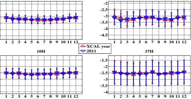
The DD biases for each channel were sorted in various ways to assure that no systematic dependency existed (e.g., by month (seasonal), time of day (day/night), with latitude, and ascending/descending segments of the orbit). Thus, finding no such effects, results presented in Figure 4-1compare the monthly average bias time-series between XCAL year and 2011, for both V- and H-pol channels at 10 and 37 GHz. Since 10 and 37 GHz are the least and most atmosphere-affected frequencies, respectively, the comparisons of the monthly DD between the two periods are representative of all channels. The results are remarked similar in that monthly DD between XCAL year (red) and 2011 (blue) in 10 V- and H-pol are nearly equal.

Figure 4-2 shows the monthly DD of ascending passes for both XCAL year (red) and 2011 (blue) by channels. Similar to Figure 4-1, the DD between these two periods match very well in all the channels except that 19 V- and H-pol channels that have relatively larger changes. However, the changes are still less than 0.2 K, which is quite acceptable. Also, the same patterns of the monthly DD are seen in descending passes.

(44)

26

Figure 4-1 Monthly average TMI-WindSat double difference bias time-series at 10 V-, 10 H, 37 V- and 37

H-pol channels, for XCAL year and 2011.

Figure 4-2 Monthly average TMI-WindSat double difference bias of ascending passes at all channels, for XCAL

year and 2011. 1 2 3 4 5 6 7 8 9 10 11 12 -1 -0.5 0 0.5 1 1.5 DD ( K ) 10V 1 2 3 4 5 6 7 8 9 10 11 12 -4.5 -4 -3.5 -3 -2.5 -2 37V 1 2 3 4 5 6 7 8 9 10 11 12 -3 -2.5 -2 -1.5 -1 -0.5 Month DD ( K ) 10H XCAL year 2011 1 2 3 4 5 6 7 8 9 10 11 12 -4 -3.5 -3 -2.5 -2 -1.5 Month 37H 1 2 3 4 5 6 7 8 9 10 11 12 -1 -0.5 0 0.5 1 1.5 DD ( K ) 10V XCAL Asc (PM) 2011 Asc (PM) 1 2 3 4 5 6 7 8 9 10 11 12 -1.5 -1 -0.5 0 0.5 1 19V 1 2 3 4 5 6 7 8 9 10 11 12 -3 -2.5 -2 -1.5 -1 -0.5 22V 1 2 3 4 5 6 7 8 9 10 11 12 -4.5 -4 -3.5 -3 -2.5 -2 37V 1 2 3 4 5 6 7 8 9 10 11 12 -3 -2.5 -2 -1.5 -1 -0.5 DD ( K ) Month 10H 1 2 3 4 5 6 7 8 9 10 11 12 -4 -3.5 -3 -2.5 -2 -1.5 Month 19H 1 2 3 4 5 6 7 8 9 10 11 12 -4 -3.5 -3 -2.5 -2 -1.5 Month 37H

(45)

27

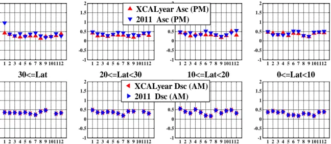
At both north and south hemispheres, the monthly DD’s of ascending and descending passes also show very good consistency between the XCAL year and 2011. In Figure 4-3, the top panel shows the DD of ascending passes through north hemisphere at 10 V-pol channel. The variation range of this case is around 0.2 K which is quite satisfactory. Moreover, the bottom panel shows that the monthly DD of descending passes at 10 V-pol channel are nearly equivalent between the two periods as well. The DD’s of ascending and descending passes in the south hemisphere present similar results, which further verifies the long-term consistency of the inter-satellite radiometric calibration between TMI and WindSat.

Figure 4-3 Monthly average TMI-WindSat double difference of asc.(top) & dsc. (bottom) passes, through north

hemisphere, at 10 V, for XCAL year and 2011.

In conclusion, this section focuses on evaluating the long-term stability of the inter-satellite radiometric calibration, between TMI and WindSat, derived from data collected during the XCAL year and 2011. The Tb biases between corresponding radiometers channels, are analyzed by: months, ascending/descending passes and latitude-based geolocation. These two one-year periods

1 2 3 4 5 6 7 8 9 101112 -1 -0.5 0 0.5 1 1.5 2 DD ( K ) 30<=Lat 1 2 3 4 5 6 7 8 9 101112 -1 -0.5 0 0.5 1 1.5 2 Month DD ( K ) 30<=Lat 1 2 3 4 5 6 7 8 9 101112 -1 -0.5 0 0.5 1 1.5 2 20<=Lat<30 1 2 3 4 5 6 7 8 9 101112 -1 -0.5 0 0.5 1 1.5 2 Month 20<=Lat<30 1 2 3 4 5 6 7 8 9 101112 -1 -0.5 0 0.5 1 1.5 2 10<=Lat<20 1 2 3 4 5 6 7 8 9 101112 -1 -0.5 0 0.5 1 1.5 2 Month 10<=Lat<20 1 2 3 4 5 6 7 8 9 101112 -1 -0.5 0 0.5 1 1.5 2 0<=Lat<10 XCALyear Asc (PM) 2011 Asc (PM) 1 2 3 4 5 6 7 8 9 101112 -1 -0.5 0 0.5 1 1.5 2 Month 0<=Lat<10 XCALyear Dsc (AM) 2011 Dsc (AM)

(46)

28

are separated by more than five years, which is very significant for evaluating the long-term consistency of TMI relative to WindSat.

The best case (10 V-pol) has an average change 0.01 K between these two periods, and this is much better than the XCAL goal of 0.1 K. The change of the worst case (19 H-pol), 0.18 K, is slightly larger than the goal but still quite acceptable. The comparison of monthly DD for TMI with respect to WindSat, between these two periods, reveals that the relative long-term stability of these two radiometers is excellent. Further, the biases are random errors that exhibit no systematic dependence on any orbital or instrument parameter.

In addition, because of the excellent stability of these two data sets, separated by a period greater than 5 years on orbit, these results also validate the long-term consistency of the CFRSL XCAL algorithm to provide a very stable transfer standard (e.g. TMI or GMI) for calibration of the precipitation measuring constellation of satellite radiometers.

4.2 Three-way Intercalibration between TMI, GMI and WindSat

R. Chen, H. Ebrahimi, and W. Linwood, “Three-way inter-satellite radiometric calibration between GMI, TMI and WindSat,” in 2016 IEEE International Geoscience and Remote Sensing Symposium (IGARSS), 2016, pp. 2036–2039 [22].

Because the radiometric transfer standard for the GPM constellation has changed to GMI, it is highly desirable to perform XCAL between GMI and TMI to link the TRMM and GPM precipitation measurements to form a multi-decadal climate dataset. Since TRMM and GPM operated together during a 13-month overlap period, it is possible to perform an inter-satellite

(47)

29

radiometric calibration; however, this activity raises the concern about the stability of this XCAL over the 17-years lifetime of TMI. Fortunately, the WindSat radiometer has existed since January 2003 and continues today; so it can provide additional XCAL with both TMI and GMI, which mitigates the long-term radiometric calibration stability issue. The purpose of this section is to extend the previous radiometric analysis between two radiometers to three radiometers, and presents a 3-way intersatellite radiometric calibration between GMI, TMI and WindSat over oceans during their 13-month of mission operations overlap (March 2014 – March 2015). This work has been published [22], and the analysis based on the latest versions of GMI V05A and TMI Tb 1B11 V8 product is exhibited in this section.

First, the gridding process described in Section 2.1.1 is applied to the Tb’s of each radiometer, where conservative filters (based upon mean values and standard deviations) are applied to exclude non-homogeneous ocean scenes (e.g., islands and weather fronts/precipitation) and other data quality issues.

Second, the gridded Tb’s of the three radiometers are collocated in ±1 or ±2-hour time window along with the geophysical parameters from GDAS. The typical coverage provided by a single orbit from each of the three sensors on May 21, 2014 is shown in Figure 4-4, and one area of triple collocations is expanded in this image. Over the 13 months of XCAL, there are approximately 33,300 boxes available for analysis.

(48)

30

Figure 4-4 Example of near-simultaneous orbits (May 21, 2014) from GMI, TMI and WindSat on a global map

(upper panel), with 3-way collocated 1°×1° boxes within ±2-hour shown in the expanded image (lower panel).

Next, theoretical (simulated) brightness temperatures, Tbsim, for each radiometer are calculated using the XCAL RTM with the collocated geophysical parameters from GDAS as inputs.

Finally, the DD technique described in Section 3.4 is used to calculate the calibration bias between each pair of radiometers, i.e., TMI to GMI, WindSat to GMI, and TMI to WindSat. Note that for each two-way comparison, the former is the target radiometer and the latter is the reference. After all boxes have been processed, the data are stratified into various categories to examine for systematic trends in the biases. For example, calibration biases are sorted monthly, as a function of latitude, and as a function of scene Tb.

(49)

31

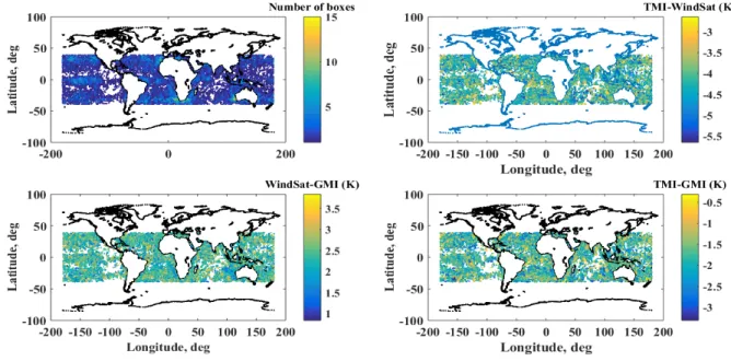
Figure 4-5 shows that the collocated boxes for all channels within a time-window of ±2 hours are approximately uniformly distributed between ±40° latitude (limited by the TRMM orbit). The upper left panel in Figure 4-5 displays the collocated boxes, with the color scale representing the number of boxes. The other 3 panels show the corresponding 3-way 37GHz V-pol DD’s plotted in color for TMI/WindSat, WindSat/GMI, and TMI/GMI.

Figure 4-5 Distribution of 3-way collocations for GMI, TMI and WindSat over oceans, within ±2-hour

time-window for the over-lap period of March 2014-March 2015. Upper left-hand panel presents the collocations,

and the color scale represents the number. The upper right-hand panel represents TMI/WindSat DD biases,

the lower panels are the WindSat/GMI and the TMI/GMI DD biases (left to right), and the color bar on the

right side of each panel indicates the value of bias.

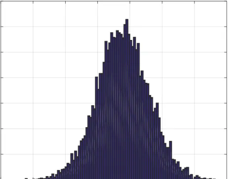
Our analysis shows that the histograms of the DD’s for all radiometers and for all channels are Gaussian, and the corresponding mean DD biases (μ) and standard deviations (std, σ) of the 3 -way XCAL are tabulated in Table 4-3 for two different temporal collocation windows. The upper

(50)

32

window panels, 86% of the mean values have a difference (∆ =│±2 hr ˗ ±1 hr│) < 0.1 K and 14% have a difference < 0.2 K. Moreover, 76% of the std differences are < 0.1 K, and the remainder

are ≤ 0.25 K. In both panels of Table 4-3, the H-pol results have higher variation than V-pol for all the three sets of DD’s; where the greatest stability occurs in the 10V channel and the most variability occurs in 19H and 37H channels. The observed stable performance of the dataset justifies using ±2 hr for the DD comparisons that follow.

Table 4-3 Double differences mean/std, upper panel is ±1 hr and lower panel is ±2 hr temporal resolution.

10V 10H 19V 19H 23V 37V 37H TMI-WS 1.04/0.33 1.15/0.31 -1.36/0.47 -1.46/0.63 -1.70/0.60 -2.29/0.42 -0.43/0.68 WS-GMI -0.38/0.20 -0.57/0.23 1.37/0.34 2.09/0.55 1.68/0.40 1.41/0.31 1.53/0.54 TMI-GMI 0.66/0.30 0.58/0.31 0.01/0.46 0.64/0.61 -0.01/0.55 -0.88/0.41 1.10/0.64 TMI-WS 1.04/0.35 1.16/0.35 -1.33/0.53 -1.44/0.76 -1.70/0.73 -2.29/0.51 -0.40/0.87 WS-GMI -0.35/0.22 -0.57/0.30 1.39/0.41 2.12/0.71 1.74/0.54 1.44/0.41 1.54/0.74 TMI-GMI 0.69/0.32 0.59/0.36 0.06/0.52 0.68/0.75 0.03/0.68 -0.85/0.52 1.14/0.87

Results presented in Figure 4-6 show that the monthly averaged values of DD radiometric bias are remarkably stable over the entire 13-month period. However, as seen from the various channels, there are significant biases between instruments. Regardless, these mean biases are not an issue because GMI is the standard for the Tb calibration, and these offsets will be applied to transform the various radiometer Tb’s to be equivalent to GMI.

(51)

33

Figure 4-6 Monthly DD of 3-way inter-calibration among GMI, TMI and WindSat by radiometer channel.

Another comparison is shown in Figure 4-7, where the DD’s are stratified by latitude, and again these results show negligible dependency on geographical location. However, note that the lowest variation occurs at 10 GHz and the highest at 19H and 37H channels, which is probably related to the DD sensitivity to the variable atmospheric conditions over the 13-month period.

(52)

34

Figure 4-7 Zonal stratification of radiometer channel DD’s for the overlap period.

Next, to examine the radiometer calibration linearity, the DD bias anomalies (means subtracted) are plotted against the corresponding reference radiometer Tb in Figure 4-8. As it was mentioned previously, it is desirable that the DD biases be constant regardless of the manner of comparison; and for most channels, the results are stable indicating that there are no systematic effects. However, for the 19H and 23V channels, the plots have a slight linear dependence, where the worst case slope (< 0.03 K/K) occurs for the 19H GMI/TMI comparison. After considerable investigation, we do not believe that this is caused by radiometer non-linearity.

(53)

35

Figure 4-8 Radiometer channel bias anomalies (DD – mean-DD) stratified by the average scene Tbobs for the

reference radiometer, which is WindSat for TMI &WindSat, and GMI for the other two radiometer

comparisons.

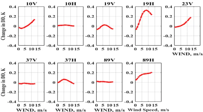
To validate this (Figure 4-8), the same DD bias anomalies are stratified by GDAS surface wind speed in Figure 4-9. For these analyses, the cross-calibration comparisons were conducted using two different ocean surface emissivity models (not shown). The results are nearly constant over the entire wind speed range for each channel. Moreover, for these channels, there is a significant atmospheric Tb component that is proportional to the integrated water vapor density. Thus, we suspect this scene dependent effect is a residual error associated with imperfect radiative transfer modeling of the water vapor resonance near 22.22 GHz, which is used in the CFRSL XCAL algorithm.

(54)

36

Figure 4-9 Radiometer channel bias anomalies (DD – mean-DD) stratified by GDAS ocean surface wind speed

for the overlap period.

During this study, DD biases and anomalies between TMI/WindSat, WindSat/GMI and TMI/GMI are characterized on a channel (frequency and polarization) basis for the 13-month overlap period, and the results are stable with small uncertainties (typically < ± 0.1 K). These 3-way collocations are uniformly distributed (spatial and temporal), and the resulting Tb DD’s, produced on individual collocated boxes, have Gaussian distributions with almost no perceived systematic effects. Thus, we believe that the histogram means are excellent estimates of the channel radiometric Tb bias, which is consistent with the GPM goal for intersatellite radiometric calibration. Moreover, it is important to note that the objective is to provide a good relative calibration between constellation radiometers, as opposed to an absolute Tb calibration. While the

(55)

37

latter is a desirable goal, we are fortunate to have GMI that appears to be extremely well calibrated and stable, which makes it an excellent calibration reference to produce the entire combined TRMM-GPM datasets and to provide the opportunity to create a consistent long-term data record [5].

Further, WindSat, which overlaps with both TMI (past) and GMI (future) will provide a much longer time series for intersatellite calibration, supporting the approach of using WindSat as the radiometric transfer standard to bridge the TRMM and GPM eras. Thus, the concern of calibration drift between GMI and TMI can be effectively mitigated by performing frequent intersatellite comparisons using WindSat to remove any long-term changes, should they exist.

Furthermore, we acknowledge that the cloud liquid water (CLW) is not well represented in GDAS numerical weather model used, and this can play a role in the RTM simulated Tb’s for the high-frequency channels. However, in a large part, this effect is mitigated by using the double difference to remove the common-mode sources of radiometric biases in the two channels considered. Moreover, future work will use microwave retrievals of CLW to evaluate its impact on DD bias and to develop more effective filters, if needed.

(56)

38

5 UNCERTAINTY QUANTIFICATION MODEL

While the CFRSL XCAL algorithm yields that the Tb bias after the composite XCAL offsets can be applied to the TMI 17-plus-year legacy Tb product, however, this is not an absolute bias. The RTM and input geophysical parameters are not perfect, hence the uncertainties due to these sources remain. In addition, the microwave sensors are with tens of kilometer resolution, the sampling process thus is subject to variability in both time and space, and further contribute to the Tb bias uncertainty. Therefore, it is necessary to quantify the uncertainty estimates considering all the uncertainty sources aforementioned and more, and to include them with the Tb bias for deriving science products into perspective.

A generic uncertainty quantification model (UQM) is developed herein, and the procedural steps involved are summarized as follows:

1) Identify sources of uncertainty.

2) Quantify uncertainty components: determine the standard uncertainty associated with each of the input quantities, including any uncertainty associated with the correction for systematic error.

3) Calculate the combined standard uncertainty from individual uncertainty.

4) Calculate the expanded uncertainty of the Tb bias by applying an appropriate coverage factor if needed.

The diagram of this model is shown in detail in Figure 5-1, and explicit explanations are provided subsequently.

(57)

39

Figure 5-1 Diagram of Uncertainty Quantification Model.

5.1 Uncertainty and Error

Before proceeding to the uncertainty estimates classification and quantification, it needs to be noted that the uncertainty in Tb is different from the Tb error. By definition, the term error is the difference between the true bias and the estimated bias. The most likely or “true” value may thus be considered as the estimated value including a statement of uncertainty which characterizes the dispersion of possible measured values. Uncertainty is caused by the interplay of errors which create dispersion around the estimated bias; the smaller the dispersion, the smaller the uncertainty

(58)

40

[23]. The uncertainty to-be-derived in this dissertation is used with a ± symbol following the Tb bias reported to the NASA PPS, indicating the uncertainty associated with the estimated Tb bias and not the error. The uncertainty of the Tb bias reflects the lack of exact knowledge of the bias due to various possible sources of uncertainty which will be discussed in Section 5.2. The following terminologies defined by [23] are used in this dissertation work:

1) The standard uncertainty is the uncertainty of the results of a measurement expressed as a standard deviation.

2) Any method for evaluation uncertainty using statistical analysis of a series of observations is call Type A evaluation of uncertainty. Any method for evaluation uncertainty by means other than the statistical analysis for a series of observations is call Type B evaluation of uncertainty.

Type A uncertainty estimates is often used in assessing random effects, and the treatment is usually a calculation of the standard deviation (STD)

𝒔𝒔(𝒗𝒗) =�∑𝒏𝒏𝒔𝒔=𝟏𝟏(𝒗𝒗𝒔𝒔−𝒗𝒗��𝒏𝒏)𝟐𝟐

𝒏𝒏−𝟏𝟏 (3)

Type B uncertainty estimation is used in systematic effects, and the treatment is to calculate the standard deviation of n mean bias of repeated experiments divided by square root of n as shown in the following equation

𝒔𝒔(𝒗𝒗𝒏𝒏) =𝒔𝒔_√𝒏𝒏(𝒗𝒗) (4)

3) Combined standard uncertainty of estimated Tb bias caused by various uncertainty sources equals to the positive square root of a sum of terms. Combined standard uncertainty may