Doctoral Dissertations University of Connecticut Graduate School
12-17-2015
Enhancing Upper-level Performance from Below:
Performance Measurement and Optimization in
LTE Networks
Ruofan Jin
University of Connecticut - Storrs, [email protected]
Follow this and additional works at:https://opencommons.uconn.edu/dissertations
Recommended Citation
Jin, Ruofan, "Enhancing Upper-level Performance from Below: Performance Measurement and Optimization in LTE Networks" (2015).Doctoral Dissertations. 981.
Below: Performance Measurement and
Optimization in LTE Networks
Ruofan Jin, Ph.D.
University of Connecticut, 2015
ABSTRACT
The current 4G LTE cellular networks provide significantly higher data rate and lower network latency than earlier generation systems. The advances provided by LTE, however, may not be fully utilized by upper-level protocols and applications. In this dissertation, we first investigate the predictability of link bandwidth in cellular networks. We then design and implement a new transport protocol that utilizes the link bandwidth prediction framework. Last, we design and implement a control-theoretic approach for adaptive video streaming for cellular networks.
For cellular link bandwidth prediction, we conduct an extensive measurement study in major US commercial LTE networks and identify various lower-level pieces of information that are correlated with cellular link bandwidth. Furthermore, we develop a machine learning based prediction framework named LinkForecast, which uses the identified lower-level information to predict cellular link bandwidth in real time. Our evaluation shows that the prediction is highly accurate: even at the time granularity of one second, the average relative error is 4.7% under static scenarios and 9.3% under highly mobile (highway driving) scenarios.
The accurate link bandwidth prediction can in turn be utilized by upper-level protocols and applications to improve their performance. We design a new transport protocol LTP that directly utilizes the real-time cellular link bandwidth prediction. Evaluations using real-world traces show that our protocol outperforms traditional TCP protocols, achieving both high throughput and low delay at the same time. Our study highlights the benefits of using radio layer information when designing higher layer protocols for cellular networks.
Last, we design and implement a PID control based scheme for adaptive video streaming in cellular networks. We start by examining existing state-of-the-art video streaming adaptation strategies from a control-theoretic point of view, and identi-fying their limitations. Motivated by the wide adoption and success of PID control in feedback control systems, we develop a PID based adaptation algorithm that op-timizes user’s perceived QoE in an online manner. Evaluations using large sets of real-world cellular traces show that our solution outperforms existing schemes under various network conditions and different user’s QoE preferences. While our approach does not require a very accurate link bandwidth prediction, its performance is further improved when using the accurate link bandwidth predictions from LinkForecast.
Below: Performance Measurement and
Optimization in LTE Networks
Ruofan Jin
M.S. Beihang University, 2010 B.S. Beihang University, 2007
A Dissertation
Submitted in Partial Fulfillment of the Requirements for the Degree of
Doctor of Philosophy at the
University of Connecticut
Ruofan Jin
Doctor of Philosophy Dissertation
Enhancing Upper-level Performance from
Below: Performance Measurement and
Optimization in LTE Networks
Presented by Ruofan Jin, B.E., M.E.
Major Advisor Bing Wang Associate Advisor Jinbo Bi Associate Advisor Donald R. Sheehy Associate Advisor Song Han Associate Advisor
Mohammad Maifi Hasan Khan
University of Connecticut 2015
My deepest gratitude goes to my major advisor, Professor Bing Wang, for her excellent guidance, continuous support, and generous encouragement throughout my doctorial study. I feel extremely lucky being one of her Ph.D. students, and having her as a constant source of wisdom, courage and skills. Her sharp insight and concise description of complicated research problems, down-to-earth attitude toward research, and her dedication have set an example of academic perfection, from which I will continue to benefit in my future career. I would also like to thank Professor Jinbo Bi, and Professor Don Sheehy, and Professor Song Han, and Professor Maifi Khan for their advice and broad knowledge. It was my great pleasure working with such intelligent and responsible professors. I would also like to thank Professor Kyoungwon Suh from Illinois State University, for his guidance on my LTE related researches.
I would like to extend my gratitude to my colleagues, Yanyuan Qin, Chaoqun Yue, Yuexin Mao, Abdurrahman Arikan, and Levon Nazaryan, for their discussions and comments in my research. My thanks also go to Wei Zeng, Xian Chen, Yuan Song, Sixia Chen, and all my friends, for their endless support whenever I needed. Last but not least, I give my deepest gratitude and love to my parents, who have been a constant source of happiness and motivation for me. Their love and support have been my inspiration to accomplish the doctoral program.
My final thanks go to my beloved wife, Ying, for her support and my beloved daughter, Elaine, whose love is worth it all.
Ch. 1. Introduction 1
1.1 LTE Basics . . . 2
1.1.1 LTE Architecture . . . 2
1.1.2 Characteristics of LTE networks . . . 3
1.1.3 Resource Scheduling . . . 5
1.2 Link Bandwidth Prediction . . . 6
1.3 New Protocol and Application Design . . . 7
1.4 Contribution of This Dissertation . . . 9
1.5 Dissertation Roadmap . . . 11
Ch. 2. LinkForecast: Predicting Cellular Link Bandwidth Using Lower-layer Information 12 2.1 Data Collection Methodology . . . 13
2.2 Data Set . . . 14
2.3 Analysis of Radio Information . . . 15
2.3.1 Signal Strength . . . 16
2.3.2 Channel Quality Indicator (CQI) . . . 19 iv
2.3.3 Resource Allocation . . . 20
2.3.4 Block Error Rate (BLER) . . . 22
2.3.5 Handover Events . . . 24
2.3.6 Time Granularity . . . 25
2.3.7 Other Phones and Networks . . . 25
2.4 Link Bandwidth Prediction . . . 28
2.4.1 Prediction Framework . . . 28 2.4.2 Prediction Performance . . . 30 2.4.3 Summary . . . 36 2.5 Discussion . . . 36 2.5.1 Carrier Aggregation . . . 37 2.5.2 Deployment Issues . . . 38 2.6 Related Work . . . 39
Ch. 3. LTP: A New Design of Transport Protocol using Link Band-width Prediction 41 3.1 LTP Design . . . 42 3.2 Protocol Evaluation . . . 44 3.2.1 Experiment Setup . . . 44 3.2.2 LTP: RTT Estimation . . . 46 3.2.3 LTP: Adjustment Factor . . . 47 3.2.4 Performance Comparison . . . 47
Ch. 4. PID Control for Adaptive Video Streaming over Cellular
4.1 Introduction . . . 53
4.2 Background . . . 55
4.2.1 Content Delivery Techniques . . . 56
4.2.2 The shift to HTTP-based Delivery . . . 57
4.2.3 Adaptive Video Streaming Strategies . . . 58
4.3 A Control Theoretic Framework for ABR . . . 60
4.3.1 DASH Standard . . . 60
4.3.2 Quality of Experience Model . . . 61
4.3.3 Video Player Dynamics . . . 63
4.3.4 Revisiting Existing Approaches . . . 64
4.3.5 PID Control for Adaptive Bitrate Streaming . . . 69
4.3.6 Improved PID Control . . . 73
4.4 Performance Evaluation . . . 75
4.4.1 Experiment Setup . . . 75
4.4.2 Performance Evaluation . . . 77
4.4.3 Sensitivity to User’s QoE Preference . . . 80
4.4.4 Sensitivity to Prediction Accuracy . . . 82
4.5 Summary . . . 84
Ch. 5. Conclusion and Future Work 85
1.0.1 Cisco Forecasts 24.3 Exabytes per Month of Mobile Data Traffic by 2019. 1 1.1.1 Illustration of LTE architecture. . . 3 1.1.2 Channel capacity and utilization of two widely used TCP variants in
LTE networks. . . 4 2.3.1 (a) Scatter plot of signal strength and link bandwidth for
highway-driving scenario. . . 17 2.3.2 Correlation coefficient between signal strength (RSRP and RSRQ) and
link bandwidth for various scenarios. . . 17 2.3.3 Correlation coefficient between signal strength (RSRP or RSRQ) and
link bandwidth for static campus scenario. . . 18 2.3.4 (a) Scatter plot of Link bandwidth and CQI in highway driving
sce-nario. (b) Correlation coefficient between CQI and link bandwidth for various scenarios. . . 20 2.3.5 Scatter plot of link bandwidth and CQI. The linear curves represent
the results from linear regression. . . 21
2.3.6 Correlation coefficient between TBS and link bandwidth for various scenarios. . . 22 2.3.7 (a) Link bandwidth and BLER versus time. (b) Scatter plot between
link bandwidth and BLER (highway driving scenario). . . 23 2.3.8 Link bandwidth and handover events. . . 24 2.3.9 Scatter plot of link bandwidth and TBS when the time granularity is 4
seconds. The linear curves represent the results from linear regression. 26 2.3.10Scatter plot of link bandwidth and MCS and nRB of the two phones
under static (campus, night time) scenario. . . 27 2.3.11Scatter plot of link bandwidth and TBS of the two phones under static
(campus, night time) scenario. . . 27 2.4.1 Bandwidth prediction accuracy when using all the factors. . . 32 2.4.2 Static scenario: (a) relative link bandwidth prediction error, (b) an
example that illustrates the benefits of using RSRQ together with TBS for prediction. . . 33 2.4.3 Highway driving scenario: (a) relative link bandwidth prediction error,
(b) an example that illustrates the benefits of using RSRQ together with TBS for prediction. . . 34 3.1.1 An illustration of our congestion control protocol that is based on link
bandwidth prediction. . . 43 3.2.1 Experiment setup. . . 45 3.2.2 Throughput for different RTT estimation methods in LTP; the shaded
3.2.3 The impact of the adjustment factor α on throughput in LTP; the
shaded area represents the bandwidth that is specified by the trace. . 46
3.2.4 Achieved throughput of LTP (α = 1.0), TCP Cubic and TCP Vegas. 52 3.2.5 Observed one-way delay of LTP (α = 1.0), TCP Cubic and TCP Vegas. 52 4.3.1 Media presentation description (MPD) in DASH. . . 60
4.3.2 BBA rate selection scheme. . . 66
4.3.3 PID Video Streaming control System Diagram. . . 71
4.4.1 Performance comparison for HSPA trace . . . 78
4.4.2 Zoomed-in results for HSPA trace set. . . 79
4.4.3 Performance comparison for LTE trace . . . 80
4.4.4 Zoomed-in results for LTE Trace Set. . . 81
4.4.5 QoE comparison for Avoid Instability setting. . . 81
4.4.6 QoE comparison for Avoid Rebuffering setting. . . 82
2.2.1 Data collected from AT&T network. . . 15
2.2.2 Data collected from Verizon network. . . 15
3.2.1 Results for static scenario. . . 50
3.2.2 Results for walking scenario. . . 50
3.2.3 Results for local driving scenario. . . 51
3.2.4 Results for highway driving scenario. . . 51
Introduction
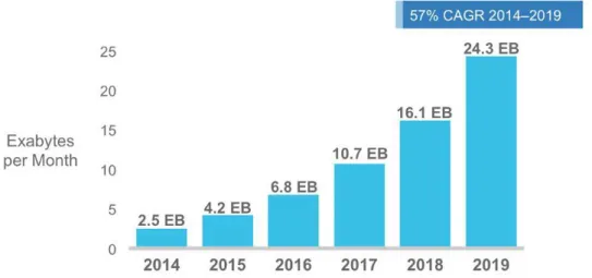
Cellular infrastructures have been evolving at a fast speed. From a recent report on global network traffic [28], it is projected that the overall mobile data traffic is expected to grow to 24.3 exabytes per month by 2019, with a compound annual growth rate (CAGR) of 57%.
Figure 1.0.1: Cisco Forecasts 24.3 Exabytes per Month of Mobile Data Traffic by 2019.
The current 4G LTE (Long Term Evolution) cellular networks provide significantly higher data rate and lower network latency than earlier generation systems. The ad-vances provided by LTE, however, may not be fully utilized by upper-level protocols and applications due to the rapidly varying cellular link conditions. For instance, a recent large-scale study of LTE networks [25] shows that, for 71.3% of the large flows, the bandwidth utilization rate is below 50%. Supporting delay-sensitive applications such as VoIP, video streaming and interactive applications in LTE networks remains to be a difficult task. With the wide deployment of LTE networks, it becomes in-creasingly important to understand cellular link characteristics, identify performance issues, and improve the performance of upper-level protocols and applications in LTE networks.
1.1
LTE Basics
1.1.1
LTE Architecture
The 3GPP Long Term Evolution (LTE) represents a major advance in cellular tech-nology. The high-level network architecture of LTE is comprised of three main compo-nents, User Equipments (UEs), the Evolved UMTS Terrestrial Radio Access Network (E-UTRAN), and the Evolved Packet Core (EPC), as shown in Fig. 1.1.1. While the core network, EPC, consists of many logical nodes, the E-UTRAN is made up of essentially just one node, the evolved NodeB (eNodeB), which connects to the UEs. Unlike some of the previous second- and third-generation technologies, LTE integrates the radio controller function into the base station. This design allows tight interac-tion between the different protocol layers of the radio access network (RAN), thus
reducing latency and improving efficiency. The eNodeB in an LTE system is respon-sible, among other functions, for managing scheduling for both uplink and downlink channels. eNodeB eNodeB X2 eNodeB X2 X2 UE E-UTRAN EPC MME S-GW P-GW
Figure 1.1.1: Illustration of LTE architecture.
1.1.2
Characteristics of LTE networks
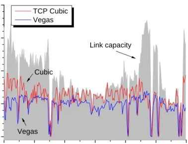
One distinguishing characteristics of cellular networks is their rapidly changing chan-nel conditions, which may cause the link bandwidths to vary in orders of magnitude within seconds. This creates two problems: low link utilization, and long delays. If too much data is sent due to an improper reaction to a reduced link capacity, a queue will be built up quickly. For instance, as shown in Fig. 1.1.2, the two widely adopted
TCP variants, Cubic (the default in Linux) and Vegas, do not perform well in LTE networks. We can observe from the figure that the link capacity (the grey area) is not effectively utilized (see Section 2.1 for details on link capacity estimation). In this example, the average utilization achieved by the two TCP variants are 74% and 45%, respectively. 0 2 0 4 0 6 0 8 0 1 0 0 1 2 0 0 1 0 2 0 3 0 4 0 T C P C u b i c V e g a s V e g a s C u b i c T h ro u g h p u t (M b p s ) T i m e ( s ) L i n k c a p a c i t y
Figure 1.1.2: Channel capacity and utilization of two widely used TCP variants in LTE
networks.
Another feature of LTE networks is that the base station, i.e., eNodeB, in the LTE networks maintains independent buffers for different clients. In downlink direction, the eNodeB maintains buffers per UE containing dedicated data traffic. Similarly, in the uplink each UE has data queues corresponding to uplink logical channels [47]. In this condition, users are rarely subject to standing queues accumulated by other users. Therefore, the latency that a UE observes primarily depends on its own packet
transmissions, independent of the actions of other users.
1.1.3
Resource Scheduling
The goal of the resource scheduling algorithm in eNodeB is to allocate the Resource Blocks (RBs) and transmission powers for each UE in order to optimize a function of a set of performance metrics. Although the LTE specification does not specify a certain scheduling algorithm, the eNodeB usually allocates resource to a UE based on many factors such as its resource scheduling algorithm, the channel condition, and the UE’s capability. A UE estimates channel quality based on various information collected from the radio channels, and reports both the channel quality and its radio capabilities (e.g., power headroom) to the associated eNodeB. Then the eNodeB allocates proper resource (e.g., the resource blocks, modulation schemes, transmission power) to the UE, based on its available resource and channel conditions. The actual algorithm used by an eNodeB for radio resource allocation is implementation dependent and not available to the public. However, in general, the resource allocation is based upon various optimization objectives such as maximizing the fairness and aggregate throughput of all UEs served by the eNodeB while observing the priorities of the UEs [8, 53]. Although it is not feasible to reverse engineer the exact resource allocation algorithm, as we will demonstrate in Sections 2.3 and 2.4, the observation of a set of radio information in a UE can shed light on the short-term behavior of resource allocation and help to predict the link bandwidth.
1.2
Link Bandwidth Prediction
One potential way of improving performance in cellular network is to predict the future link conditions. It is demonstrated that an accurate link bandwidth prediction can benefits upper-layer protocols and applications significantly [39, 57, 54, 15]. Along this line, existing studies [54, 53] have tried to infer the link bandwidth by modeling uncertain dynamics of the network path using network level information (e.g., historic throughput, delay, loss rate, etc.). However, we observed that the highly dynamic network environment often makes these prediction approaches less accurate.
While the rapidly varying link conditions in LTE networks pose challenges to upper-level protocols and applications, unique characteristics of cellular networks also present opportunities. Specifically, for a cellular link, a rich set of high-fidelity lower-layer (PHY/MAC) information is being collected by the user device and the base station, and is exchanged between these two entities in real time (used routinely for scheduling purposes). The lower-layer information provides important insights on the cellular link bandwidth, and can be used for link bandwidth prediction, which can in turn be utilized by upper-level protocols and applications to improve their performance.
The predictability of cellular link capacity, along with the fact that last-hop cel-lular links (i.e., access links of clients) remain to be the bottleneck [29, 16], indicates that bandwidth of an end-to-end path can be largely estimated in real time. This opens the door for completely new transport protocol and application designs.
In this dissertation, we conduct an extensive measurement study in a commercial LTE network and identify five types of lower-level information that is correlated with cellular link bandwidth. Furthermore, we develop a machine learning based
prediction framework, LinkForecast, which uses the identified lower-level information to predict link bandwidth in real time. Our evaluation shows that the prediction is highly accurate: even at the time granularity of one second, the average relative error is 4.7% under static scenarios and 9.3% under highly mobile (highway driving) scenarios; the relative errors are reduced to 1.9% and 2.2% respectively when the time granularity is four seconds.
1.3
New Protocol and Application Design
The accurate link bandwidth prediction can in turn be utilized by upper-level pro-tocols and applications to improve their performance. We explore new designs for transport protocols in LTE networks that directly utilize the real time link band-width prediction. Evaluation using real-world traces demonstrates that our protocol outperforms traditional TCP protocols, achieving both high throughput and low de-lay at the same time. Compared with a recent transport protocol that is designed for cellular networks, our protocol achieves similar or better performance while our pro-tocol is much simpler and does not require long training period. Our study highlights the benefits of using radio layer information when designing higher layer protocols for cellular networks.
Meanwhile, real-time entertainment (comprised of streaming video and audio) continues to be the largest traffic category on virtually every network. For instance, during the evening peak hours (8pm - 1am EDT), well over 50% of US Internet traffic is video streamed from Netflix and YouTube [4]. Among the video streaming traffic, an increasing fraction is driven by video consumption on mobile phones and tablet
devices on mobile networks, thanks to a significantly higher link bandwidth enabled by the 4G LTE networks.
Many recent studies have highlighted that the user-perceived Quality of Experi-ence (QoE) plays a critical role for Internet video streaming application [18, 32]. The key metrics involves average video quality, duration of rebuffering, number of video quality switches, etc. However, due to the rapidly varying link condition in cellular network, it remains to be a big challenge to provide users with a seamless multime-dia experience with high QoE. Specifically, achieving good QoE in adaptive video streaming requires maximizing the average video bitrate, minimizing the amount of rebuffering and bitrate variation. These three optimization goals are at odds with each other, and are extremely difficult to balance in cellular networks with highly dynamic bandwidth.
Many recent studies have provided solutions for tackling this problem (e.g. [26, 50, 30, 17, 27, 55]). Some studies try to find better ways to estimate the future throughput [30], some try to augment the throughput prediction with buffer informa-tion [17, 50] and some other [27] even argue against capacity estimainforma-tion and propose to use buffer occupancy solely. (A more detailed overview of related work can be found in Section 4.2.3).
While previously studies have shown key limitations of state-of-art solutions and proposed a wide range of heuristic solutions, most of the solutions are heuristic and there is still a lack of understanding about their inherent mechanisms and how to properly tune their system parameters. In order to further understand the adaptive video streaming in cellular network, we begin by formulating the existing approaches in a control-theoretic framework. Then we analyze their system characteristics and identify their limitations. After that, we design a PID based feedback control
frame-work and investigate the system behavior by conducting comprehensive evaluations under numerous controller settings and various real-world cellular traces. By exam-ining the evaluations results, we provide a guideline for tuning the adaptive video streaming system. Following the guideline our system shows that the system be-havior is consistent with the design and it outperforms state-of-art video streaming solutions. We hope our work can shed some light on the video adaptation design for the cellular networks.
In this dissertation, we design and implement a PID control based approach for adaptive video streaming in cellular networks. We start with analyzing existing state-of-the-art video streaming approaches from a control-theoretic point of view, and identifying their limitations. Motivated by the wide adoption and success of PID control in feedback systems, we develop a PID based strategy that optimizes QoE in an online manner using both buffer occupancy and estimated link bandwidth at the client. Evaluation using a large set of real-world cellular traces demonstrates that our solution outperforms existing schemes in a wide range of settings. Our approach does not require accurate link bandwidth prediction. On the other hand, its performance can be further improved with accurate link bandwidth prediction using LinkForecast.
1.4
Contribution of This Dissertation
The contributions of this dissertation are as follows.
• We investigate various information from the radio interface of a mobile device, and identify several key parameters that have strong correlation with cellular link capacity. Our study significantly expands the scope of existing studies [46,
15, 49] that only focus on one or two types of information.
• Based on the key parameters that identified, we develop a machine learning based prediction framework, LinkForecast, that uses the identified radio infor-mation to predict link bandwidth in real-time. Evaluations demonstrate that our prediction is highly accurate: even at the time granularity of one second, the average relative errors are 4.7% and 6.9% under static and walking scenarios, and are 4.3% and 9.3% under local and highway driving scenarios, respectively. The relative errors are even lower for larger time granularity.
• We design a new congestion control protocol for LTE networks. To the best of our knowledge, this is the first transport protocol that directly utilizes real-time link bandwidth prediction. Extensive evaluation using large-scale traces from a commercial LTE network demonstrates that our protocol achieves both high throughput and low delay. It significantly outperforms traditional TCP protocols in both link utilization and latency.
• We examine existing state-of-the-art video streaming adaptation schemes from a control-theoretic point of view, and identify their limitations. Motivated by the wide adoption and success of PID control in feedback systems, we develop a PID based adaptation algorithm that optimizes QoE in an online manner using both buffer occupancy and link bandwidth information at the client. Evaluations using a large set of real-world cellular traces demonstrate that our solution outperforms existing schemes under various network conditions and different user’s QoE preferences. While our approach does not require a very accurate link bandwidth prediction, its performance is further improved when using the accurate link bandwidth predictions from LinkForecast.
1.5
Dissertation Roadmap
The remainder of this dissertation is organized as follows.
In Chapter 2, we describe our work on predicting cellular link bandwidth using lower-layer information. In Section 2.1 and Section 2.2, we describe the data collection methodology and the data set used throughout this dissertation, respectively. In Section 2.3, we investigates the correlation between various radio layer information and cellular link bandwidth. In Section 2.4 we presents the design and performance of our link bandwidth prediction framework LinkForecast. And in Section 2.5, we discuss a couple of practical issues.
In Chapter 3, we present our work on designing a new transport protocol LTP that utilizes link bandwidth prediction from LinkForecast. In Section 3.1, we describe the design of LTP. And in Section 3.2, we evaluate the performance of LTP under various scenarios.
In Chapter 4, we design a PID-based control algorithm for adaptive video stream-ing over cellular networks. In Section 4.1 we introduce the background of adaptive video streaming and PID control. In Section 4.2, we describe the related work on video streaming. In Section 4.3 we formulate the problem, examine existing solutions from a control-theoretic point of view, and propose our PID-based video streaming adaptation algorithm. In Section 4.4, we evaluate the performance the proposed solution under a wide range of settings.
LinkForecast: Predicting Cellular
Link Bandwidth Using Lower-layer
Information
As mentioned in Chapter 1, the rapidly varying link conditions in LTE networks pose challenges to upper-level protocols and applications. On the other hand, unique characteristics of cellular networks also present opportunities. The lower-layer infor-mation provides important insights on the cellular link bandwidth, and can be used for link bandwidth prediction, which can in turn be utilized by upper-level protocols and applications to improve their performance.
In this chapter, we first explore the correlation between various lower layer in-formation and cellular link bandwidth. For this purpose, we conduct an extensive measurement on two major US commercial LTE networks to identify a set of infor-mation from both network layer and radio layer that is correlated with cellular link bandwidth. After that, we explore the predictability of cellular link bandwidth by
developing a machine learning based prediction framework named LinkForecast. We demonstrate that LinkForecast provides accurate cellular link bandwidth in real-time.
2.1
Data Collection Methodology
We collect data from two largest commercial LTE networks in the US. Specifically, we collect two types of information, cellular link bandwidth and lower layer information, simultaneously. These two types of information will be used for the following two purposes : (i) they will be used to study the correlation between link bandwidth and various radio information to identify key parameters that can be used for link bandwidth prediction in Section 2.3; and (ii) the radio information will be used to predict link bandwidth and be compared with the collected link bandwidth (treated as the ground truth) to evaluate the accuracy of the prediction framework in Section 2.4. We next describe how we obtain these two types of information. Link bandwidth represents the bandwidth that is available to a UE over the cellular link. It is not directly perceivable, and has to be obtained through active measurement. We use a purposely written program to send a certain amount of data that can saturate the link while not causing very long queuing delays. While the link is saturated, we use a packet sniffer to record the network traffic.
Lower layer information is available at a UE. However, currently commodity UEs do not expose the information to the operating system at a fine granularity (see more discussion in Section 2.5). We use QxDM (Qualcomm eXtensible Diagnostic Moni-tor), a tool developed by Qualcomm [44], to record various radio information in real time for phones with Qualcomm chipsets. Specifically, to record QxDM traces, we
connect a phone using a USB cable to a laptop that runs QxDM. QxDM commu-nicates with the phone through a diagnostic port and records the traces, where the various radio information is logged periodically, with the intervals varying from tens of milliseconds to hundreds of milliseconds.
Furthermore, in order to make sure that the extra data collection overhead does not affect the normal operation of the phone. We measured the CPU usage on a phone when collecting radio information with QxDM, and find that QxDM does not cause any noticeable increase in CPU usage. In other words, collecting radio information in real-time does not affect the performance of the phone.
2.2
Data Set
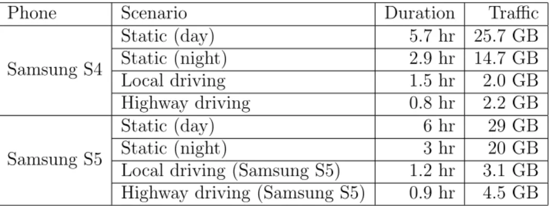
We have performed extensive measurements during a period of 15 months (from July 2014 to October 2015) in two major US commercial LTE networks, AT&T and Verizon. The data are collected using seven different phones, Samsung S3, S4, S5, Note 3 and HTC M8 in AT&T network, and Samsung S4 and S5 in Verizon networks, at locations in three states CT, NY and NJ in the US.
We collected around 50 hours of data, and 200 GB of traffic traces under a wide range of scenarios, including different times of a day, different locations (residential, campus, office, etc.), and different movement speed (stationary, walking, local driving, and highway driving). Tables 2.2.1 and 2.2.2 list the majority of the data collected in AT&T and Verizon networks, respectively. For clarity, only the data collected by Samsung Note 3 in AT&T network is marked with time. Because the traces were collected at different times and places, the measurements cannot be used to compare
Table 2.2.1: Data collected from AT&T network.
Phone Scenario Duration Traffic
Samsung Note 3 Static (day) 3.3 hr 9.8 GB Static (night) 2.5 hr 7.8 GB Walking (day) 1.5 hr 4.3 GB Walking (night) 0.7 hr 2.2 GB Local driving 1.2 hr 4.7 GB Highway driving 1.4 hr 9.8 GB HTC M8 Static (day) 6.6 hr 16.5 GB Static (night) 2.7 hr 15.5 GB Local driving 0.6 hr 2.1 GB Samsung S3, S4, S5 various scenarios 4.5 hr 21.2 GB
Table 2.2.2: Data collected from Verizon network.
Phone Scenario Duration Traffic Samsung S4 Static (day) 5.7 hr 25.7 GB Static (night) 2.9 hr 14.7 GB Local driving 1.5 hr 2.0 GB Highway driving 0.8 hr 2.2 GB Samsung S5 Static (day) 6 hr 29 GB Static (night) 3 hr 20 GB Local driving (Samsung S5) 1.2 hr 3.1 GB Highway driving (Samsung S5) 0.9 hr 4.5 GB
different commercial services head-to-head.
2.3
Analysis of Radio Information
We analyze all the available LTE related physical and MAC layer information provided by QxDM. In the following, we describe a set of parameters that are identified to be correlated with cellular link bandwidth. For each parameter, we first describe the intuition why the correlation might be significant, and then present quantitative measurement results.
We use multiple time granularity (i.e., time unit ∆ is 1, 2, 4, or 10 seconds) when analyzing the correlation between radio information and link bandwidth. We only present the results based on the time granularity of one second; the results for other time granularity are similar. For clarity, we first present the results based on the data collected from Samsung Note 3 in AT&T network (see Table 2.2.1). Then we briefly describe the results in other settings.
2.3.1
Signal Strength
Three types of signal strength information are available from the radio interface: RSSI (Received Signal Strength Indicator), RSRP (Reference Signal Received Power), and RSRQ (Reference Signal Received Quality). RSSI represents the total power a UE observes across the whole band, including the main signal and co-channel non-serving cell signal, adjacent channel interference and the noise within the specified band. RSRP is the linear average (in watts) of the downlink reference signals across the channel bandwidth. It measures the absolute power of the reference signal. RSRQ is defined as (N ·RSRP)/RSSI, where N is the number of resource blocks over the measurement bandwidth. In other words, RSRQ indicates what the portion of pure reference signal power is over the whole E-UTRAN power received by the UE.
Since RSSI does not measure specifically the link between a UE and eNodeB, we focus on the other two types of signal strength information, namely, RSRP and RSPQ. We observe that RSRP is correlated with link bandwidth in all cases. Fig. 2.3.1(a) is a scatter plot of RSRP and link bandwidth under the highway driving scenario, where each point represents the average bandwidth over one second and the corre-sponding average RSRP over that second. We observe that when RSRP is very low,
(a) RSRP (b) RSRQ
Figure 2.3.1: (a) Scatter plot of signal strength and link bandwidth for highway-driving
scenario. 0 10 20 30 −0.5 0 0.5 1 Time lag (s) Correlation coefficient Highway driving Local driving Walk (daytime) Static (daytime) (a) RSRP 0 10 20 30 −0.2 0 0.2 0.4 0.6 0.8 Time lag (s) Correlation coefficient Highway driving Local driving Walk (daytime) Static (daytime) (b) RSRQ
Figure 2.3.2: Correlation coefficient between signal strength (RSRP and RSRQ) and
0 10 20 30 0.2 0.25 0.3 0.35 Time lag (s) Correlation coefficient RSRP RSRQ (a) daytime 0 10 20 30 0 0.1 0.2 0.3 0.4 Time lag (s) Correlation coefficient RSRP RSRQ (b) night time
Figure 2.3.3: Correlation coefficient between signal strength (RSRP or RSRQ) and link
bandwidth for static campus scenario.
link bandwidth tends to be low as well (see lower left corner); similarly, when RSRP is very high, link bandwidth tends to be high as well (see upper right corner). Sim-ilar correlation is observed between RSRQ and link bandwidth (see scatter plot in Fig. 2.3.1(b)).
Fig. 2.3.2 plots cross correlation between signal strength (RSRP or RSRQ) and link bandwidth under various scenarios. Specifically, for each scenario, we obtain two time series,{bi}and{ri}, wherebi andri are respectively the average link bandwidth
and signal strength (RSRP or RSRQ) during the ith second. We explore the cross correlation with lag l, i.e., between bi+l and ri, where l = 0,1, . . . ,30 seconds. We
observe that the correlation is significant even at the lag of tens of seconds except for the walking scenario (where the correlation is only significant at the lag of a few sec-onds). In general, we observe that the correlation between RSRP and link bandwidth is comparable to that between RSRQ and link bandwidth. This observation differs from the observation in [15], which shows that RSRQ is more correlated with link bandwidth than RSRP. The difference might be because the results in [15] are from
a more congested 3G network. We also observe that the correlation between signal strength (RSRP or RSRQ) and link bandwidth is larger for high mobility scenarios (local and highway driving) compared to low mobility scenarios (static and walking). Fig. 2.3.3 plots the correlation coefficients between signal strength and link band-width in a static setting in a university campus. Figures 2.3.3(a) and (b) differ in that one is collected during daytime, while the other is collected in night time, both of a total duration of 2800 seconds. Interestingly, we observe that the correlation between RSRQ and link bandwidth is close to zero. This is the only scenario where RSRQ is not correlated with link bandwidth. Inspecting the trace, we think this might be because during night time, RSRQ is fairly stable while link bandwidth fluctuates over time.
2.3.2
Channel Quality Indicator (CQI)
As the name implies, CQI is an indicator carrying the information on the quality of the communication channel. It is a 4-bit integer (i.e., the value is between 0 and 15), and is determined by a UE [9]. LTE specification does not specify how a UE calculates CQI. In general, a UE takes into account multiple factors (e.g., the number of antennas, signal-to-interference-noise-ratio (SINR), the capability of its radio) when calculating CQI. The calculated CQI is reported to the eNodeB, which performs downlink scheduling accordingly.
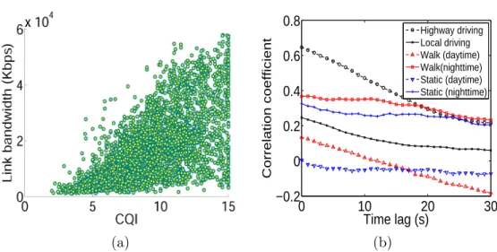
We observe that CQI is correlated with link bandwidth in most cases. As an example, the correlation can be visually observed in the scatter plots in Fig. 2.3.4(a), which is for highway driving scenario. In general, the correlation between CQI and link bandwidth is the highest under highway driving scenario, and is lower under
(a) 0 10 20 30 −0.2 0 0.2 0.4 0.6 0.8 Time lag (s) Correlation coefficient Highway driving Local driving Walk (daytime) Walk(nighttime) Static (daytime) Static (nighttime) (b)
Figure 2.3.4: (a) Scatter plot of Link bandwidth and CQI in highway driving scenario.
(b) Correlation coefficient between CQI and link bandwidth for various scenarios.
other scenarios.
Fig. 2.3.4(b) plots the correlation coefficient of CQI and link bandwidth under various scenarios. We find that in one scenario (static on campus during daytime), the correlation between CQI and link bandwidth is very low. For the other cases, the correlation is significant even when the lag is up to a few or tens of seconds.
2.3.3
Resource Allocation
In LTE networks, time-frequency resources are allocated in units of resource blocks (RBs). A resource block consists of 12 consecutive sub-carriers, or 180 kHz, for the duration of one slot (0.5 ms). The scheduling decision of an eNodeB for a UE includes a specific Modulation and Coding Scheme (MCS) and the number of resource blocks (nRB). The first parameter, MCS index is in the range of 0 to 31. It summarizes the modulation type and the coding rate that are used in the allocated RBs. Typically, a higher MCS index offers a higher spectral efficiency (which translates to a higher
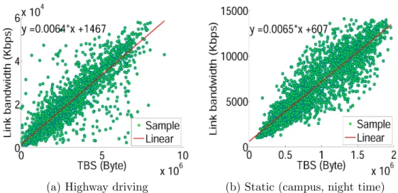
(a) Highway driving (b) Static (campus, night time)
Figure 2.3.5: Scatter plot of link bandwidth and CQI. The linear curves represent the
results from linear regression.
potential data rate), but requires a channel with better quality to support it. The second parameter, nRB, determines how many resource blocks are allocated to a UE. With the MCS index and nRB, the Transport Block Size (TBS) can be uniquely determined by looking up the mapping tables defined in 3GPP 36.213 [9]. In general, a higher value of MCS and a larger nRB yield a larger TBS, and thus lead to higher link bandwidth.
We observe that TBS is strongly correlated with link bandwidth in all the cases. In addition, the relationship between bi and T BSi is very similar in all the cases, where bi and T BSi denote respectively the average link bandwidth and the aggregate TBS
in theith second. Fig. 2.3.5 shows the scatter plot between bi and T BSi in two very
different scenarios, one corresponding to highway driving and the other corresponding to static scenario (on a university campus during night time). Both plots show a strong linear relationship betweenbi and T BSi. The linear regression models for the
two cases have similar coefficients. Of all the cases, we have bi =αT BSi+β, where α is between 0.0059 and 0.0070, and β is between 600 and 1500 (which is very small
0
10
20
30
0.2
0.4
0.6
0.8
1
Time lag (s)
Correlation coefficient
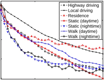
Highway driving Local driving Residence Static (daytime) Static (nighttime) Walk (daytime) Walk (nighttime)Figure 2.3.6: Correlation coefficient between TBS and link bandwidth for various
scenarios.
given that bi can be up to tens thousands of Kbps).
Fig. 2.3.6 plots the correlation coefficient between TBS and link bandwidth for various scenarios. We observe very high correlation (above 0.8) when the lag is a few seconds. Even when the lag is tens of seconds, the correlation is still significant.
2.3.4
Block Error Rate (BLER)
Hybrid-ARQ (HARQ) is used in LTE networks to achieve higher efficiency in trans-mission and error correction. It uses 8 stop-and-wait processes to transmit data. Once a packet is sent from a particular process, the process will be in active state and will not process other packets until it receives an ACK or NACK. If a NACK is received, then a retransmission will be initiated. If too many retransmissions happen, the eNodeB has to adjust the modulation and coding scheme. Specifically, HARQ Block Error Rate (BLER) is defined as the number of erroneous blocks divided by
0 5 0 1 0 0 1 5 0 2 0 0 2 5 0 3 0 0 0 1 0 2 0 3 0 4 0 L i n k b a n d w i d t h B L E R T i m e ( s ) Li nk b an dw id th ( M bp s) 0 5 1 0 1 5 2 0 B L E R ( % ) (a) 0 10 20 30 0 2 4 6x 10 4 BLER (%) Link Bandwidth (Kbps) (b)
Figure 2.3.7: (a) Link bandwidth and BLER versus time. (b) Scatter plot between link
bandwidth and BLER (highway driving scenario).
the total number of blocks that are sent. The target BLER is typically 10% [9]. If the actual BLER is larger than 10% (e.g., due to weak signal strength or interference), the link must be switched to a lower speed, and vice versa.
Fig. 2.3.7(a) plots link bandwidth and BLER over time for a five-minute long trace. We see the BLER is fluctuating around 10%; when the BLER is high, the link bandwidth is low. Fig. 2.3.7(b) is a scatter plot between link bandwidth and BLER under the highway driving scenario. We observe that most of the BLER values are between 0.05 and 0.1. When BLER is above 0.1, the link bandwidth tends to be low. On the other hand, when BLER is below 0.1, the link bandwidth is in a wide range. As a result, the cross correlation between BLER and link bandwidth is not significant (figure omitted).
0 2 0 4 0 6 0 8 0 1 0 0 0 1 0 2 0 3 0 4 0 L in k b a n d w id th ( M b p s ) T i m e ( s ) H a n d o v e r
Figure 2.3.8: Link bandwidth and handover events.
2.3.5
Handover Events
A handover is performed when a UE moves from the coverage of one cell to the coverage of another cell in the connected state. Unlike the case in UMTS, there are only hard handovers in LTE networks, i.e., a UE cannot communicate with multiple eNodeBs simultaneously. Therefore, there will be a short interruption in service when a handover happens. The impact of the LTE handover procedures on the user experience depends very much on the type of the application that is being used. For instance, a short interruption in a large file downloading may not be even noticeable, while an interruption in a delay-sensitive application (e.g., VoIP, video streaming, interactive online gaming) can be very disruptive. We use the changes in serving cell ID to detect the handover events.
Fig. 2.3.8 plots a sample trace of link bandwidth where handover events are marked as red dots. It shows that an instant decrease in bandwidth when handover happens. We represent handover events as a binary time series{hi}, wherehi = 1 if there exists a handover event in the ith second andhi = 0 otherwise. Again let{bi}represent the
{hi}and {bi}does not reveal significant correlation in any of the scenarios (the most
significant correlation is under highway driving where the correlation under lag 1 is around -0.1). This might be because of the infrequency of handover events.
2.3.6
Time Granularity
The results presented above using time granularity of 1 second. The results under other granularity (2, 4, and 10 seconds) are consistent with those under one second granularity. We still observe that RSRP, RSRQ, CQI, TBS, BLER and handover events are correlated with link bandwidth in various scenarios, and TBS has the highest and most consistent correlation across all the scenarios.
Fig. 2.3.9 shows the scatter plot between link bandwidth and TBS in highway driving and static (on a university campus during night time) scenarios. We again observe a strong linear relationship between these two quantities. The linear regres-sion models for the two scenarios (and also other scenarios) have similar coefficients. Compared with the results using one second as granularity (see Fig. 2.3.5), the points are closer to the linear line because the amount of randomness is lower when using a larger granularity. In addition, the slope of the line is around one fourth of the value under one second granularity since the TBS is the aggregate over 4 seconds (approximately four times as the aggregate over one second).
2.3.7
Other Phones and Networks
The analysis above is based on the traces collected from Samsung Note 3 (denoted as Phone 1) in AT&T network. In order to understand whether the correlation still holds for different phones, we pick a much older and less powerful Samsung S3 (denoted as
(a) Highway driving (b) Static (campus, night time)
Figure 2.3.9: Scatter plot of link bandwidth and TBS when the time granularity is 4
seconds. The linear curves represent the results from linear regression.
Phone 2) on purpose, and collect traces in both static and walking scenarios. While Phone 2 achieves a similar average throughput as Phone 1 (5.3 Mbps versus 5.7 Mbps in static scenario and 7.7 Mbps versus 7.9 Mbps in walking scenario). We observe that Phone 2 in general uses many more resource blocks and slower modulation and coding schemes. Figures 2.3.10(a) and (b) show the scatter plots for MCS and nRB, respectively, for the two phones. From the figure, we can observe that Phone 2 uses much lower MCS than Phone 1. In other words, the sending speed for each resource block is much slower than Phone 1. However, in order to compensate for the lower MCS, we also observe that Phone 2 is allocated as many as 50 resource blocks, while Phone 1 gets at most 25. In some sense, eNodeB allocates more resource to Phone 2 to compensate for the inferior radio capability.
Fig. 2.3.11 shows the scatter plot of link bandwidth and TBS for the two phones. As explained earlier, TBS reflects the combined effect of both MCS and nRB. We observe that the two phones actually exhibit a very similar correlation between link bandwidth and TBS. For Phone 2, the correlations between other factors and link
(a) MCS (b) nRB
Figure 2.3.10: Scatter plot of link bandwidth and MCS and nRB of the two phones
under static (campus, night time) scenario.
Figure 2.3.11: Scatter plot of link bandwidth and TBS of the two phones under static
bandwidth are similar as those for Phone 1 (figures omitted).
We also evaluate the correlation results for other phones and Verizon network. Overall, the results exhibit very similar trends. For instance, when using Samsung S5 on Verizon network, at lag 1, the correlation coefficients of RSRP and link bandwidth range from 0.42 to 0.60 for various scenarios, for RSRQ and CQI, the correlation coefficients range from 0.31 to 0.52, and 0.32 to 0.61, respectively.
2.4
Link Bandwidth Prediction
After an extensive correlation analysis of radio layer information, we explore the predictability of cellular link bandwidth. Specifically, we develop a machine learning based framework calledLinkForecast that predicts link bandwidth in real-time using radio information. In the following, we first describe the prediction framework, and then evaluate the performance of LinkForecast.
2.4.1
Prediction Framework
LinkForecast adopts a random forest [13] based prediction model. The reason for choosing the random forest model is that it is a state-of-the-art prediction model that requires low memory and computation overhead. In addition, it ranks the importance of the variables, and hence can be used to identify dominantly important factors. Compared to using a single regression tree, random forest uses the average of multiple trees (we use 20 trees), and hence is less sensitive to outliers in the training set and does not suffer from overfitting. We note that it is possible to use other prediction techniques, which is left as future work.
LinkForecast adopts a discrete time system t = 1,2, . . . where each time unit is ∆, and the prediction is at the granularity of ∆. When a set of n radio information is used for link bandwidth prediction, the input vector x to LinkForecast is of the form {x1
t, x2t, . . . , xnt}, where xit is the ith information during the interval between
t−1 tot, i= 1, . . . , n. To obtain xi
t, we may need to average or aggregate multiple
samples of this information from the radio interface. Specifically, if the sampling interval isδ, then approximately ∆/δsamples will be used to obtainxi
t. For the radio
information we identified in Section 2.3, the sampling interval varies from 20ms to 320ms. Therefore, when using ∆ = 1 sec, the number of samples used varies from 3 to 50. The output of the LinkForecast is the predicted link bandwidth ˆbt for time t. LinkForecast may also use more historical information to predict ˆbt. For instance, it
may use {x1
t−k, x2t−k, . . . , xnt−k}, . . . ,{x1t, x2t, . . . , xnt} to predict ˆbt, where k ≥ 1. Our
results below only use{x1
t, x2t, . . . , xnt}.
The prediction is in an online manner, using a prediction model that is obtained beforehand. Specifically, the prediction model is learned from a training set that is obtained offline. Since regression cannot predict beyond the range in the training set, the range of the training set needs to be sufficiently large. We discuss how we select training set later. In general, assuming variation in the data set (which is the case for cellular networks), the training set can be chosen as a sufficiently long trace. Note that since the training is done offline, the size of the training set does not affect the performance of online prediction. In fact, random forest incurs very low memory and computation overhead. Even when using thousands of seconds long training trace and six types of radio information (i.e., n = 6), the computation time on a commodity laptop is negligible.
2.4.2
Prediction Performance
We evaluate the performance of LinkForecast in each category listed in Table 2.2.1. Specifically, for each category, we use the first 90% of the data as training set, and the remaining 10% of the data as testing set. After that, we consider four broad categories: static, walking, local driving and highway driving, concatenate all the traces in each category, and for each category, use the first 90% of the data as training set, and the remaining 10% of the data as testing set. Since there are multiple ways of concatenating the data, we also evaluate the results under different ways of concatenation. For each testing set, we feed the radio parameter traces from QxDM to LinkForecast, and then compare the predicted bandwidth with the ground truth link bandwidth to obtain prediction accuracy. Unless otherwise specified, the results in the following consider the four broad categories using data from Samsung Note 3 on AT&T network (the prediction accuracies for other phones and networks are similar).
In the following, we first present the evaluation results when using all six types of radio information identified in Section 2.3, namely, TBS, RSRP, RSRQ, CQI, BLER and handover events, for prediction. We then evaluate the performance when using only the dominant factors identified by the random forest approach. At the end, we evaluate the sensitivity of prediction accuracy to training data. The time granularity ∆ is set to 1, 2, 4, and 10 seconds, motivated by the needs of transport protocols and delay-sensitive applications [54, 57, 39].
Using All Factors
LinkForecast provides accurate prediction in all the scenarios. Specifically, when ∆ = 1 second, the average relative error for static, walking, local driving, and highway driving scenarios are 4.7%, 6.9%, 4.3%, 9.3%, respectively. For larger ∆, the relative errors are even smaller (because the variation under larger ∆ is smaller). For instance, when ∆ = 4 second, the average relative error for these four scenarios are reduced to 1.9%, 2.8%, 1.4%, and 2.2%, respectively.
Figures 2.4.1 (a) and (b) plot the predicted bandwidth versus the ground-truth bandwidth under static and highway driving scenarios, respectively. In the static scenario, the average downlink bandwidth is 6.5 Mbps, while in the highway driving scenario, the average link bandwidth is 16.5 Mbps. For each scenario, the range of the ground-truth bandwidth is equally divided into 20 bins. For each bin, we obtain the mean and standard deviation of the predicted bandwidth (with corresponding ground-truth bandwidth falling in the bin). The shaded areas in the figures represent the contour surrounding the mean minus the standard deviation and the mean plus the standard deviation. In addition, the error bars mark the 95th and 5th percentiles. We observe that the predicted bandwidth matches well with the actual bandwidth.
For all the scenarios, the random forest approach consistently ranks TBS as the most important factor. This is perhaps not surprising given the very high correlation between TBS and link bandwidth across all the scenarios. In addition, RSRQ and RSRP are ranked high in importance, closely followed by CQI. The other two factors, BLER and handover events, are ranked lower maybe because of our data set. For other data set (e.g., with very frequent handover under high mobility [34]), handover events may become a more important factor.
(a) Static scenario. (b) Highway driving scenario.
Figure 2.4.1: Bandwidth prediction accuracy when using all the factors.
Using Dominant Factors
We next compare the performance when only using the dominant factors with the performance when using all the factors. In the interests of space, we only present the results under the static and highway driving scenarios; the results under the other two scenarios have similar trend. For each scenario, we first present the results when only using the highest-ranked factor, TBS, and then add one or more other factors and explore how they improve the prediction accuracy.
Fig. 2.4.2(a) plots the cumulative distribution function (CDF) of the relative pre-diction errors for the static scenario. When using TBS alone, 90% of the relative errors are within 10%. The performance is slightly worse than that when using all the factors (where 90% of the relative errors are within 6%). However, we see from the figure that using TBS alone can lead to overestimation, which can be detrimental to higher level protocols [29]. When using both TBS and RSRQ, the overestimation is significantly reduced, as shown in one example in Fig. 2.4.2(b) (the circles mark the places where adding RSRQ reduces overestimation). Using TBS together with other
- 2 0 - 1 0 0 1 0 2 0 3 0 4 0 0 . 0 0 . 2 0 . 4 0 . 6 0 . 8 1 . 0 C D F R e l a t i v e e r r o r ( % ) A l l T B S _ o n l y (a) 0 5 0 1 0 0 1 5 0 2 0 0 2 5 0 3 0 0 3 5 0 1 . 5 3 . 0 4 . 5 6 . 0 7 . 5 T h ro u g h p u t (M b p s ) T i m e ( s ) T B S + R S R Q T B S o n l y (b)
Figure 2.4.2: Static scenario: (a) relative link bandwidth prediction error, (b) an
example that illustrates the benefits of using RSRQ together with TBS for prediction.
factors can also help to reduce overestimation; the effect is less significant compared to that using RSRQ.
The results under the highway driving scenario have similar trend (see Fig. 2.4.3). When using TBS alone, 80% of the relative errors are within 18%. When using all the factors, 80% of the relative errors are within 11%. Again, using RSRQ together with TBS leads to less overestimation.
Sensitivity to Training Data
To further verify the universality of our prediction model, we evaluate the sensitivity to training data in the following five settings (without otherwise specified, we used the data from Samsung Note 3 on AT&T network). The first setting iscross-scenario
prediction, where we use the data collected in one scenario as training data, and then use the prediction model thus learned to predict link bandwidth in another scenario. The second setting is cross-phone prediction, where we use the data collected on one
- 4 0 0 4 0 8 0 1 2 0 0 . 0 0 . 2 0 . 4 0 . 6 0 . 8 1 . 0 C D F R e l a t i v e e r r o r ( % ) A l l T B S o n l y (a) 0 5 0 1 0 0 1 5 0 2 0 0 2 5 0 3 0 0 3 5 0 3 6 9 1 2 1 5 1 8 B a n d w id th ( M b p s ) T i m e ( s ) T B S + R S R Q T B S O n l y (b)
Figure 2.4.3: Highway driving scenario: (a) relative link bandwidth prediction error, (b)
an example that illustrates the benefits of using RSRQ together with TBS for prediction.
phone to learn a prediction model, and then use it to predict link bandwidth for another phone. The third setting is the cross-period, i.e., the training and testing sets are from two time periods several months apart. And the fourth is cross-carrier
prediction, i.e., the training and testing sets are from two different carriers. And lastly the fifth setting iscross-location prediction, where the training and testing sets are from two different states.
Cross-Scenario Prediction. For each scenario, we use the data collected from all the other scenarios as the training data. We thus create four pairs of training and testing sets given the four scenarios (static, walking, local driving, and highway driving) that we consider. When using highway driving scenario as the testing set, and the data collected in the other three scenarios as training data. We observe that the prediction is very accurate — 90% of the relative errors are within 8.8%. The results under the other three pairs of training and testing sets are similar.
to different phones, we conducted “cross-phone” prediction test. Specifically, we use the data collected from one phone as training data, and the data collected on another phone as testing data. When using data collected on HTC M8 as training set and using the data collected from a Samsung phone as testing set, 80% of the relative errors are within 9.7%. Mean is 7.1%. The results for other combinations are similar and are thus omitted.
Sensitivity to Time. To confirm the data is not time-sensitive, we conduct a “cross-time” test. Since our data is collected over a period of 17 months, we choose two far apart datasets — one from July 2014 and the other from Nov. 2015. When we use the first dataset as training data, 80% of the relative errors are within 9.8%, with a mean error of 7.3%. When we use the second dataset as the training data, 80% of the relative errors are within 10.4% with a mean error of 8.1%. Again we observe accurate prediction results, indicating that our results are not sensitive to time.
Sensitivity to Carrier. Another question remains is whether our model can be applied to different network carriers. To answer the question, we perform a “cross-carrier” test. Specifically, we compile two datasets: one is from all the data collected from the phones on Verizon network, and the other is from all the data collected from the phones on AT&T network as the testing set. When we use the Verizon data as training set, 80% of the relative errors are within 10.8%, with a mean error of 8.5%. When we use the AT&T data as training set, 80% of the relative errors are within 11.2%, with a mean error 9.1%. In both case, our model achieves a good prediction accuracy.
Sensitivity to Location. In the end, we verify if our model is insensitive to different locations. As we described, our data is collected from three different states in the
US. In our test, we separate the data collected from CT and NJ and treat them as two datasets. When we use the NJ data as training set, 80% of the relative errors are within 12.5%, with a mean prediction error of 10.1%. When using the CT data as training set, 80% of the relative errors are within 10.5%, with a mean is 8.1%. The prediction result indicates that our prediction model is not tied to any specific locations.
2.4.3
Summary
In this section, we designed and implemented a machine learning based framework named LinkForecast that predicts link bandwidth in real-time using both network layer information and radio information. Our evaluation shows that it achieves a very good prediction accuracy in various scenarios. And we demonstrate that our prediction scheme is not sensitive to training data, and can be applied to different phones, different time, different carriers and different locations.
2.5
Discussion
In this section, we discuss a couple of practical issues, one related to using our ap-proach when a UE is served simultaneously by multiple base stations (a practice that has started to be adopted by commercial carriers [3, 7]), and the other related to the implication of our study in practice.
2.5.1
Carrier Aggregation
In most of our measurements, a UE is served by a single base station at a given point of time. In some cases, we observe carrier aggregation (CA) [52], where a UE is served by both two base stations (i.e., primary and secondary base stations) simultaneously. CA is defined in LTE Advanced (3GPP Release 10) in order to increase the bandwidth, and thereby increase the bitrate [52, 5]. It has been launched in major LTE networks as of December 2014 and the coverage of CA in the major LTE networks continues to be expanded [3, 7]. We observe CA in a residential area, which is occasionally served with CA.
In the presence of CA, we obtain radio parameters as the average of both the primary and secondary base stations. We observe that the correlation between TBS and link bandwidth is very high (similar as that under the case without CA). In the traces where CA is present in some portion of the trace, we obtain a time series on the number of base stations that are being used in each second (i.e., the value is either 1 or 2, depending on whether CA is present or not), and find that this time series has strong correlation with the time series of link bandwidth.
Our prediction approach can be applied to the case with CA by adding information related to the secondary base station and the number of base stations. We have verified that using TBS alone still provides accurate link bandwidth prediction in the presence of CA. Due to limited amount of trace, we leave further investigation to future work.
2.5.2
Deployment Issues
We use QxDM to gather fine-granularity (at the interval of tens of or hundreds of milliseconds) radio information with the goal of exploring the performance space. Specifically, the goal is to identify what information is critical for accurate link band-width prediction and at what granularity the information is useful. A natural question is, since such information is not yet accessible on commodity phones (indeed we have to resort to QxDM), how to use our approach in practice.
We make the following two comments. First, a recent trend is that lower-layer information becomes increasingly accessible. Specifically, current mobile processors and chipsets (e.g., Qualcomm Snapdragon processors) provide ways to read various parameters from the radio interface of a mobile device in real time; mobile operating systems are exposing more radio related APIs (e.g., Android has included APIs that provide multiple signal strength related information); and manufacturers are provid-ing lower level information to users (e.g., the service menu on Samsung smartphones). We hope that our results can serve to accelerate the trend in making radio informa-tion accessible at mobile devices. Secondly, our results indicate that even a small set of information at coarse granularity is useful for obtaining accurate link bandwidth prediction. Even if not all radio information is made available at fine granularity in the near future, we hope our results can incentivize the practitioners to make a small set of critical radio information accessible at coarse granularity.
Last, it is worth mentioning that the prediction performance of LinkForecast can-not be directly used as an indicator for transport or application layer performance. For instance, if a low bandwidth link is mis-predicted as having high bandwidth, it is very likely to cause a transport protocol or an application to send more data than
the link can handle, and thus creates a large queue, which may take seconds to be drained. We will investigate using LinkForecast in designing transport protocols in Chapter 3.
2.6
Related Work
Bandwidth estimation has been studied extensively in wired networks (e.g., [20, 19]) and wireless LANs (e.g., [33, 35]). The study in [31] demonstrates that existing band-width estimation techniques for wired networks and wireless LANs are not effective in cellular networks. Xu et al. [54] develop a system interface called PROTEUS that forecasts future network performance (throughput, loss, and one-way delay) based on current measurements, and integrate PROTEUS with real-time communication appli-cations. Winstein et al. [53] use packet inter-arrival time to infer link bandwidth and further determines the number of packets that can be transmitted. The techniques in [54, 53] rely on network metrics.
The studies in [46, 15, 49, 40, 39] use low-layer radio information to predict link bandwidth. Schulman et al. find that signal strength (RSSI) is correlated with link bitrate and power consumption, and propose an energy-aware scheduling algorithm for different workloads [46]. Chakraborty et al. develop a SVM (Support Vector Machine) based technique that categorize bandwidth into two classes (high and low bandwidth), and propose a technique for UEs to coordinate cellular background transfer in an efficient manner [15]. Sorous et al. find that signal strength and throughput are correlated to some extent [49], and demonstrate that measurement of throughput at a server can be used to reveal user location. Margolies [40] et al. generate throughput
prediction for a mobile device based on the observation that the signal quality of a device is remarkably reproducible for multiple drives on the same path. While our work also uses radio information, it differs from the above studies in that it investigates an extensive set of radio-layer information, and constructs a prediction model that predicts in realtime link bandwidth in LTE networks.
The work that is closest to ours is [39]. Our study is independent and in parallel to [39], and differs from [39] in several important aspects. The study in [39] uses CQI and DRX (discontinuous transmission) ratio to predict link bandwidth in HSPA+ networks. The prediction is by looking up a mapping table at a base station. Since the mapping table is vendor implementation dependent, the authors propose to use crowdsourcing to obtain the mapping table at each base station. Our goal is to identify a comprehensive set of radio information that can be used to provides highly accurate link bandwidth prediction, and then use it as an upper bound to identify a small set of information that can achieve most of the gains in LTE networks. We use machine learning techniques for prediction and demonstrate that our approach is not sensitive to training data. In addition, using an extensive data set, we quantify the correlation between various radio information and link bandwidth under different scenarios.
Several studies investigated the relationship between radio status and performance at an end device. Liu et al. studied the interplay between wireless channels and applications in CDMA networks [37]. To capture the radio information, Vallina-Rodriguez et al. implemented a tool named RilAnalyzer [51], which can record the radio connection status and application behaviors. While our study also considers radio information and higher-layer performance, it differs in scope from them.
LTP: A New Design of Transport
Protocol using Link Bandwidth
Prediction
Chapter 2 demonstrated that lower layer information can be used to accurately predict cellular link band-width in real time. This actually opens a door for completely new transport protocol designs. Indeed, there is a fundamental mismatch between knowing the approximate end-to-end bandwidth and the design principle of TCP that probes for bandwidth (and then reacts when congestion happens). Therefore, a new paradigm is needed for upper layer protocol and application designs.
In this chapter, we investigate the benefits of using LinkForecast to upper-layer protocols. Specifically, we design congestion control protocol for LTE networks that directly utilizes real-time link bandwidth prediction from LinkForecast. We refer to the protocol as LTP (LinkForecast based Transport Protocol). Our intention is to demonstrate the benefits of knowing link bandwidth to the design of transport
protocols. We compare the performance of LTP with existing transport protocols using the cellular traces collected from commercial LTE networks.
3.1
LTP Design
LTP directly utilizes the prediction results from LinkForecast to avoid probing for bandwidth as in standard TCP protocols. On the other hand, our protocol can be built incrementally on top of a standard TCP protocol by adjusting the congestion window through the client’s advertised receive window (see details below). Fig. 3.1.1 illustrates our protocol. In this protocol, radio layer information is collected from the radio interface, which will be used by the bandwidth predictor to predict band-width in real time. The predicted bandband-width will be fed to the congestion controller, which will in turn adjust the congestion window of TCP. Specifically, consider a TCP flow between a server and a client. At each point of time, the congestion window of the TCP flow is the minimum of the client’s advertised receive window and the server’s congestion window. Therefore, by adjusting the advertised receive window, the congestion window can be indirectly controlled by the client.
Consider a UE that is connected to a LTE network. When sending data from the UE (i.e., the data flows uplink), the UE uses LinkForecast to predict the bandwidth in the uplink direction. Let Bu
t denote the predicted uplink bandwidth at time t.
Then LTP sets the congestion window at time t to
α·B
u
t ·RTTt
MTU·Nt
, (3.1.1)