The Impact of a Feed-In Tariff on
Wind Power Development in Germany
Claudia Hitaj, Michael Schymura,
and Andreas Löschel
The Impact of a Feed-In Tariff on
Wind Power Development in Germany
Claudia Hitaj, Michael Schymura,
and Andreas Löschel
Download this ZEW Discussion Paper from our ftp server:
http://ftp.zew.de/pub/zew-docs/dp/dp14035.pdf
Die Dis cus si on Pape rs die nen einer mög lichst schnel len Ver brei tung von neue ren For schungs arbei ten des ZEW. Die Bei trä ge lie gen in allei ni ger Ver ant wor tung
der Auto ren und stel len nicht not wen di ger wei se die Mei nung des ZEW dar.
Dis cus si on Papers are inten ded to make results of ZEW research prompt ly avai la ble to other eco no mists in order to encou ra ge dis cus si on and sug gesti ons for revi si ons. The aut hors are sole ly
Claudia Hitaj
*,
Michael Schymura
†, and
Andreas Löschel
‡— May 23, 2014 —
Abstract—
We estimate the impact of a feed-in tariff for renewable power on wind power investment in Germany at the county level from 1996-2010 controlling for windiness and access to the electricity transmission grid. After the Renewable Energy Law (EEG) was passed in 2000, the feed-in tariff became linked to wind power potential, such that more windy locations received a lower incentive per unit of output. We find that a 1e-cent/kWh increase in the feed-in tariff rate would increase additions to capacity at the national level by 764 MW per year from 1996-2010 or 1,528 MW per year from 2005-1996-2010. We analyze counterfactual scenarios, in which a uniform incentive is offered instead of the wind-dependent EEG incentive. Significantly more wind power plants are installed along the northern coastal counties in the uniform incentive scenario. We find that while the uniform incentive results in greater total wind power output per installed capacity, the EEG is ultimately more efficient by achieving 1% greater wind power output per euro and 3.7% greater reductions in power sector emissions per euro. In addition, we find a significant response from investors to an EEG provision that shifted the cost of transmission system upgrades from wind power developers to grid operators in 2000. The lack of a signal on scarcity of transmission capacity has likely resulted in a distribution of wind power plants that makes suboptimal use of existing infrastructure, necessitating investment in new transmission corridors.
Keywords:Wind power, feed-in tariff, electricity transmission
JEL-Classification:Q0, Q42, Q50
The analysis and conclusions expressed here are those of the authors and may not be attributed to the Economic Research Service or the US Department of Agriculture. All re-maining errors are fully attributable to the authors.
*Economic Research Service, United States Department of Agriculture, E-mail: [email protected]
†Centre for European Economic Research (ZEW), E-mail: [email protected].
‡Centre for European Economic Research (ZEW) and University of Heidelberg, E-mail: [email protected]
1 I
NTRODUCTIONR
ENEWABLE POWERin Germany enjoyed broad public support when a feed-in tariff for re-newables was instituted in 1991. Industry response to the feed-in tariff was strong with installed wind power capacity growing nearly three-hundred-fold from 0.1 GW in 1991 to 29.1 in 2011. Supporting renewables and promoting energy efficiency are part of a broader energy policy, theEnergiewendeor transformation of the energy system, which includes phasing out nuclear power by 2022.With the Energiewende Germany has become a global player in the green technology sec-tor. The motivations behind the Energiewende are not only economic. According to BMU [2013] there is a popular consensus that Germany has an ethical and cultural obligation to show the world that economic competitiveness can be reconciled with sustainable develop-ment in a leading industrial nation. Despite this basic public support for the Energiewende, criticism is mounting as renewable penetration in the grid increases. Companies threaten to relocate operations outside of Germany, citing rising energy costs. Citizens complain about wind turbines and transmission lines located close to their homes. Electricity experts see an increasing risk of blackouts as investment in transmission infrastructure lags behind in-vestment in renewable power. The European Union has investigated whether the feed-in tariffs for renewable power and industry exemptions for paying them constitute illegal subsi-dies. Economists and policymakers question whether the cost of supporting renewables has outpaced the benefit of reduced emissions and whether subsidizing renewable power makes sense after the inception of the European Union emissions trading scheme (ETS) in 2005.
The Energiewende had humble beginnings. Shortly after reunification of West and East Germany, the Law on Feeding Electricity into the Grid or Stromeinspeisungsgesetz (StrEG) came into effect in 1991 to promote the production of renewable power through a feed-in tariff (FIT) guaranteed over the first twenty years of the lifetime of the plant. The idea behind the law was to support renewables to reduce emissions in the power sector (1) and to prevent large electricity transmission companies from underpaying for electricity from small power producers (2) [Berchem, 2006]. The success of the StrEG took industry and government by surprise. Installed wind power capacity grew from 106 MW in 1991 to 4435 MW in 1999. In 2000, the German government passed the Renewable Energy Law or Erneuerbare Energien Gesetz (EEG). It maintained the structure of supporting renewables with a 20-year FIT, but clarified the allocation of interconnection costs and linked the level of the FIT to the windiness of plant locations, such that less windy locations receive a higher FIT. This location-specific FIT is an unusual component of the EEG that we investigate in our paper.
Despite continued public discussion of the Energiewende in general and renewable power in particular, basic facts about the impact of these subsidies on wind power development in Germany remain unexplored. Büsgen and Dürrschmidt [2009] review a 2007 progress report on the EEG by the Federal Ministry for the Environment, Nature Conservation and Nuclear Safety. They draw conclusions from estimates of the amount of electricity remunerated under the FIT policy and the amount of emissions reductions, but they do not estimate the addition-ality of the EEG - that is they assume no development of renewable power in the absence of the EEG. Frondel et al. [2010] estimate the net present cost of EEG support for renewables and provide a critique of the law, but they too do not account for additionality, nor do they allow for a location-specific FIT in the case of wind power. Diekmann et al. [2008] provide
a comprehensive analysis and critique of the EEG, focusing on the impacts on the economy as a whole, specific industries, and the power sector. However, they too do not specifically quantify the impact of the EEG on investment in wind power.
Several studies have focused on the co-existence of the EEG and ETS, since any emission reductions achieved through the EEG in Germany would lead to a reduction in the ETS permit price and a corresponding increase in emissions. Traber and Kemfert [2009] estimate the impact of the EEG on electricity prices and emissions in the context of the ETS. They decompose the effects of the FIT into a substitution effect, triggered by the replacement of conventional by renewable sources, and a permit price effect induced via the ETS. They find that the EEG caused German consumer prices to increase by 3%, producer prices to decrease by 8%, and emissions to decrease by 11%. However, European emissions are reduced only by 0.5%, since other European countries increase emissions due to the FIT-induced drop in the permit price. Frondel et al. [2010] come to a similar conclusion. Ideally, the ETS cap would need to be adjusted according to the level of FIT support for renewables in member countries. It has also become increasingly clear that the subsidies for renewable power have led to a much higher than expected investment in renewables with a correspondingly higher than anticipated cost. Büsgen and Dürrschmidt [2009] estimated that the cost of the EEG to the consumer would peak at 1.5 cent/kWh around 2020, while in reality it has reached 6.24 cent/kWh in 2014.
This paper is the first study to quantify the effect of feed-in tariffs on additions to installed wind power capacity across German counties from 1995-2010, building on a similar analysis by Hitaj [2013] for the United States. The econometric analysis takes advantage of the fact the feed-in tariffs in Germany have varied both over time and across counties, allowing us to distill how great a portion of the expansion in wind power is due to the EEG as opposed to other factors. Previous studies have ignored this issue of additionality. Control variables include windiness, electricity transmission grid density, county GDP, population density, land value, voting rates for the Green Party (to capture environmental consciousness), and tech-nological advances in wind turbines.
We find that the StrEG and EEG FIT had a significantly positive effect on wind power development. A 1e-cent/kWh increase in the initial FIT rate would cause capacity additions at the national level to increase by 764 MW per year over the study period of 1996-2010 and 1,528 MW per year in 2005-2010. While the importance of the level of the FIT increased over time, the importance of ease of access to the electricity grid declined. We find that grid den-sity has a positive effect on wind power plant installations only in 1996-1999. In 2000, the EEG shifted the burden of transmission system upgrade costs from wind power developers to grid operators, after which point grid density no longer has a significant effect on wind plant installations. We also find evidence that the regulatory change in 2004 requiring locations to meet a minimum windiness standard to remain eligible for the FIT had a significant ef-fect, with ”just” eligible locations experiencing greater wind power investment than ineligible counties.
Finally, our study allows us to further investigate a unique feature of the Renewable En-ergy Law. Beginning in 2000, the level of the feed-in tariff varied across locations depending on average wind speeds, such that less windy locations received higher subsidies per unit of output. The revenue a wind power plant owner receives is equal to the product of output and the FIT rate. As output increases with windiness, the FIT decreases as well by design. This
means that revenue initially increases linearly with output and then gradually flattens out, such that locations with medium and high levels of windiness receive the same amount of revenue. This set-up induces a more uniform distribution of wind plants across the country than under a non-varying FIT.
At first glance, providing higher incentives at less windy places seems sub-optimal. The same amount of installed wind power capacity would produce a lower amount of power in the uniform case than in the clustered case. However, less money is spent on subsidizing investment in very windy areas, which might experience the same level of development with a lower incentive. Whether the overall lower cost combined with the decrease in output results in a larger or smaller output per euro is unclear a priori. In addition, power system-level emissions rates vary across the country, and different distributions of wind power plants result in different levels of emission reductions per euro.
Based on the estimates from the regression analysis, we analyze counter-factual scenar-ios, in which a uniform national incentive is offered as opposed to the EEG incentive that depends inversely on windiness. We demonstrate how the total capacity, power output, and spatial distribution of wind plants differ across these scenarios, and also estimate their cost-effectiveness. We find that the EEG performs slightly better than a uniform national incen-tive in terms of cost-effecincen-tiveness, achieving a 1% greater power output from wind plants per euro spent and a 3.7% greater emission reduction per euro spent than the equivalent uniform incentive. The EEG would likely perform even better if transmission congestion were taken into account, as congestion is more of an issue in areas with a high concentration of wind power plants. Thus, we find that the cost savings from linking the FIT level to windiness are substantial enough to make up for the associated reduction in output, though the overall improvement in efficiency is only minor.
2 B
RINGINGW
INDP
OWERO
NLINEDespite its small land mass, Germany was the world leader in installed wind power ca-pacity until 2007, when it was overtaken by the United States and later China. In relative terms Germany outperforms both countries, producing 7.4% of its electricity supply from wind power plants in 2012 compared with 3.4% and 2% for the United States and China, respectively [BMWi, 2013, EIA, 2013, BNEF, 2013].1
The German government has offered generous feed-in tariffs for renewables for the past two decades, resulting in a rapid expansion of wind power in Germany and making Germany particularly suitable for a study to quantify the effects of feed-in tariffs on investment in wind power.
The profitability of a new wind plant depends on a location’s wind speed profile, avail-ability of government incentives, and access to the transmission grid. The benefit of a wind plant in terms of its contribution to abatement depends on the emissions rates of the conven-tional power plants its output substitutes for. This section first presents the evolution of the feed-in tariff for wind power and then provides an overview of the structure of the German
1The share of electricity generated from wind power is greater in four other countries: 30% in Denmark, 18% in Spain and Portugal, and 16% in Ireland EIA [2013].
power sector, focusing on interconnection procedures for wind power plants and power sector emissions.
2.1 Policy Incentives for Wind Power from 1991 to 2010
The federal incentive program for wind power began in 1991 with the Stromeinspeisungs-gesetz (StrEG) or Law on Feeding Electricity into the Grid. The law required utilities to purchase electricity from wind power plants at a fixed price (feed-in tariff) equal to 90% of the average retail price of electricity from two years prior and also guaranteed access to the electricity grid through interconnection. Wind power plants received the feed-in tariff (FIT) for a period of 20 years. Installed wind power capacity increased significantly from 55 MW in 1990 to 4435 MW in 1999, supplying 1% of electricity in 1999.
The StrEG was replaced in 2000 by the Erneuerbare Energien Gesetz (EEG) or the Re-newable Energy Sources Act. Similar to the StrEG, wind power plants receive a FIT over 20 years, but the EEG stipulates a separate higher tariff for the first 5 years. The initial period with the higher tariff is extended for those wind power plants with an expected output less than 150% of reference output2 by 2 months for each 0.75% of the reference output, by which the expected output falls short of 150% of the reference output. Thus, a wind power plant with an expected output of 142.5% would receive the higher initial FIT for an addi-tional 2*(150-142.5)/0.75 = 20 months. This stipulation means that the EEG incentive varies across locations according to wind power potential, with less windy locations receiving more federal support per unit of output than more windy locations. Table 1 summarizes the federal incentives for wind power and installed capacity from 1991 to 2011.
The EEG revision in 2004 lowered the FIT for wind power, specified an annual FIT de-gression rate of 2%, and excluded wind power plants with an expected output less than 60% of reference output from receiving the FIT. The latter clause ensures that wind power develop-ment does not occur in locations with very low wind resources. The 2009 revision raised FIT rates, lowered the degression rate to 1%, and introduced a 0.5e-cent/kWh system-services-bonus during the initial period for wind power plants that fulfill certain technical require-ments for grid integration of intermittent resources, such as flicker control, harmonics, and low-voltage ride through.
The costs of the FIT scheme during the first decade under the StrEG were borne by utilities, which could pass them on the customers through rate increases. Beginning with the EEG in 2000, costs were distributed directly to end-use consumers through a nationally uniform EEG surcharge on electricity bills. Energy-intensive companies facing international competition can apply to be exempted from the surcharge.
2.2 Structure of the Electricity Sector: Deregulation and Market Power
Deregulation of the electricity sector began in 1998 with the Energy Industry Act or Energiewirtschaftsgesetz (EnWG), which stipulated that independent power producers have open access to the transmission grid. The vertically integrated power companies controlling generation, transmission and distribution resources were required to keep separate records of these three activities. No regulatory agency was created to oversee the liberalization. Un-2Reference output varies according to the type of turbine and is defined as the output over five years given an average wind speed of 5.5 m/s at 30m above ground.
Table 1: Wind Power Feed-In Tariffs and Installed Capacity
Law Year Initial Incentive Base Incentive Installed Capacity
(e-cent/kWh) (e-cent/kWh) (MW) StrEG (1990) 1991 8.49 106 1992 8.45 174 1993 8.47 326 1994 8.66 618 1995 8.84 1,121 1996 8.80 1,549 1997 8.77 2,089 1998 8.58 2,877 1999 8.45 4,435 EEG (2000) 2000 9.10 6.19 6,097 EEG (2004)a 2004 8.70 5.50 16,623 2005 8.53 5.39 18,390 2006 8.36 5.28 20,579 2007 8.19 5.17 22,194 2008 8.03 5.07 23,826 EEG (2009)a 2009 9.20b 5.02 25,703 2010 9.11b 4.97 27,191 2011 9.02b 4.92 29,071
a Wind plants with an expected output less than 60% of reference output are not eligible
to receive the feed-in tariffs.
b Wind plants that fulfill certain technical requirements for grid integration (flicker
con-trol, harmonics, low-voltage ride through) receive an additional 0.5e-cent/kWh System-Services-Bonus in the initial period.
der this setup, transparency and enforcement remained an issue, particularly since only an on-the-books separation was required. Independent power producers negotiated agreements with power companies that owned the transmission infrastructure in order to transport their electricity on the grid. However, without a regulator, large power companies could still prior-itize transmission of electricity from their own generation assets over that from independent power producers.
The process of separating generation from transmission activities began in 1998 and was not completed by 2010, the end of the study period of this paper. In 2005, the law was changed to create a regulatory agency (Federal Network Agency or Bundesnetzagentur), and large power companies were required to separate their transmission and distribution ac-tivities from their generation acac-tivities within the company (divestment was not required). Germany’s power market is very concentrated, as four power companies, RWE, EnBW, E.ON and Vattenfall, produced 82% of electricity in 2010 [EC, 2012]. Beginning only in 2010 did three of the four power companies sell or partly sell their subsidiaries controlling the trans-mission system.3 These large companies held market power, at least in principle, since they 3In response to inquiries from the European Commission for Competition, the four largest power companies, RWE, EnBW, E.ON and Vattenfall, moved their transmission system
op-would have been able to favor transmitting electricity from their own generators over elec-tricity from independent power producers. Indeed, Weigt and von Hirschhausen [2008] find realized wholesale electricity prices to be greater than competitive benchmark prices, indi-cating the presence of market power. Figure 7 in the Appendix depicts the control areas of the four transmission system operators.
2.3 Interconnection and Dispatch
The system of feed-in tariffs instituted in 1991 opened up the market to independent power producers of renewable energy, since the price of electricity was set by the government and paid for by the consumer. However, the StrEG makes no provisions for which party bears the costs of interconnection. The EEG in 2000 clarifies that renewable power plants must bear the cost of connecting to the nearest economically and technically feasible interconnec-tion point in the grid, but the transmission operator must pay for any necessary grid upgrades to accommodate the new plant. Despite this provision, interconnection costs can be the sub-ject of negotiation, since in some cases it is difficult to distinguish where interconnection costs end and grid upgrade costs begin [Leprich et al., 2008].
The EEG stipulates that transmission operators must give renewable power plants imme-diate priority for interconnection. However, the law does not elaborate on what “immeimme-diate” constitutes, nor does it provide for sanctions in the case of non-compliance [Leprich et al., 2008]. Despite the fact that the costs of the feed-in tariff can be passed on to consumers, transmission operators incur additional indirect costs, such as transactions costs and system upgrade costs (that are not directly passed on to the consumer), when renewable power plants interconnect to their grid [Leprich et al., 2008]. This can lead to tensions between TSOs and renewable power plant operators.
Ideally, a large shift in energy policy as it is codified in the EEG and envisioned in the Energiewende requires coordination between power plant developers and grid operators at the national level, so that investment in generation and transmission infrastructure can be jointly optimized. In reality, no such coordination existed until the Power Grid Expansion Act (Energieleitungsausbaugesetz) was passed in 2009 and the Network Development Plan (Netzentwicklungsplan) began in 2011.
The system of shallow interconnection fees, in which the grid operator pays for system upgrade costs, combined with priority dispatch for renewable power and a fixed feed-in tariff that does not take into account transmission constraints or system demand means that re-newable power plant developers receive essentially no location signals that would allow for optimal use of the existing transmission infrastructure. Without a location signal, chances are high that renewable power plants locate in suboptimal locations, while transmission op-erators are required by law to provide swift interconnection and incur the cost of system upgrades. Only recently is the Federal Network Agency directly involved in coordinating transmission expansion at the national level. Joint optimization may have reduced total costs significantly - Phillips and Middleton [2012] estimates costs could have been reduced by up to 50% in Texas.
erations into newly created subsidiaries. In 2010, E.ON and Vattenfall sold their respective subsidiaries, Tennet TSO and 50Hertz Transmission, and in 2011 RWE sold a majority share in its subsidiary Amprion. TransnetBW remains a full subsidiary of EnBW.
Expansion of the grid is necessary to transport electricity produced in the windy North to the energy intense industries and population centers located in the South and West of Ger-many. Building new transmission lines is a lengthy and contentious process, particularly in a country that is as densely populated as Germany. Companies in the German wind indus-try consider insufficient grid expansion to be the major threat to the expansion of renewable energies in Germany [Stegen and Seel, 2013].
2.4 Intermittency and Power Sector Emissions
Since wind power is intermittent and cannot be perfectly predicted, transmission opera-tors must keep back-up capacity online to make up for unexpected shortfalls in output. The costs associated with this back-up capacity are generally low4but increase with higher levels of wind power penetration. Fast-ramping natural gas plants are better suitable than slow-ramping coal plants for counter-balancing fluctuations in wind plant output at the sub-hourly and hourly level. If wind powe ris more likely to replace natural gas than coal, this is bad news in terms of emissions reductions, since coal plants emit roughly twice as much carbon dioxide than natural gas plants do.
Natural gas is more expensive than coal, which is another reason why wind power is more likely to substitute for power from natural gas rather than coal plants. As more renewable power plants come online, the price of electricity decreases, since plants with high marginal costs, such as natural gas, drop further down in the merit order and are dispatched less frequently.5
The expense of natural gas and its fast ramp rate mean that natural gas power plants produce less power with increased penetration of wind power in the grid. Traber and Kemfert [2011] find that at current wind power supply levels the incentives to invest in flexible natural gas power plants capable of counter-balancing the intermittent supply of wind power are insufficient. This slows down the transition to a low-carbon power sector, since the new generation of conventional plants in Germany is predominantly coal.
The benefit of renewable power plants depends heavily on location. First, some areas of the grid may experience frequent transmission constraints, in which renewable power is cur-tailed in favor of conventional power located closer to demand centers. Second, the abatement achieved by a renewable power plant varies across locations and depends on the configura-tion of the grid [Hitaj, 2014]. A subsidy for renewable power does not take this varying rate of abatement into account.
3 D
ATA3.1 Wind Power Installations
This paper investigates the effect of policy incentives on wind power development in Ger-many from 1995 to 2010 across all 402 counties (Kreise). The dependent variable is additions
41-4e/MWh or 5-10% of the wholesale value of wind energy at wind energy penetrations of up to 20% of gross demand [EWEA, 2009]
5This increases the cost of the feed-in tariff program, which pays plants the difference between the electricity price and the feed-in tariff.
to installed capacity (if any) in county i in year t. Data on wind power installations were obtained from EEG/KWK-G [2013]. Of the 6,030 county-time observations, 2,173 or 36 % had positive additions to wind power capacity. Only 19 counties (5 %) had already installed wind power plants in 1995.
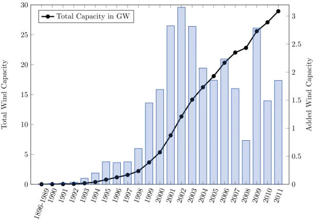
Figure 1 depicts the development of installed wind power over time. There has been a steady increase in installed capacity with marked jumps after the institution of the EEG in 2000 and changes to the policy in 2004 and 2009. The slowing economy had a negative impact on investment in 2008. 1896-1989 1990 1991 1992 1993 1994 1995 1996 1997 1998 1999 2000 2001 2002 2003 2004 2005 2006 2007 2008 2009 2010 2011 0 5 10 15 20 25 30 T otal Wind Capacit y Total Capacity in GW 0 0.5 1 1.5 2 2.5 3 Added Wind Capacit y
Figure 1: Total and Added Capacity
Figure 2 depicts cumulative installed windpower capacity from 1995-1999, 2000-2004, and 2005-2010 by county windpower potential. Clearly, the best (most windy) sites are devel-oped first with investment shifting towards less-windy counties in 2000-2010, when greater incentives per unit of output were offered under the EEG than under the StrEG.
0 500 1000 1500 2000 2500 3000 3500 4000 4500 5000 5500 6000 6500 50 100 150 200 250 300 350 400 450 Windpower potential (kWh/m2) Cum ulativ e installed capacit y (in MW) Counties (1999) 2000 - 2004 2005 - 2010 Ineligible line
Figure 2: Cumulative additions to installed capacity by period and windpower
potential
3.2 Wind Power Potential
Data on wind power potential at 200m cell resolution were obtained from the German Weather Service [DWD, 2013]. The distribution of wind speeds at a particular location is most commonly approximated with the Weibull distribution. The DWD has calculated the Weibull parameters for each cell based on wind data collected at 218 stations from 1981 to 2000, taking into account elevation and local topography. Based on these Weibull parameters, the DWD has estimated the expected power output over five years in kWh per m2 of rotor
swept area, assuming a hub height of 80 m, a start speed of 3 m/s, and a stop speed of 25 m/s. The county-level spatial average of this five-year expected electricity output in kWh/m2is the
measure used in this paper to account for varying wind power potential across counties. This measure offers a much finer gradation than the more commonly used wind power class or average wind speed. In addition, as the relationship between wind speed and power output is non-linear, expected wind power output can more readily be incorporated into the linear regression equation than either wind power class or average wind speed.
Figures 3a and 3b show how wind power potential and installed capacity are concen-trated in Northern Germany. However, population and economic activity are centered in the southern and western parts of Germany (Figures 3c and 3d). This mismatch between de-mand for electricity and the location of wind resources will intensify in the future, as the government is set to phase out nuclear power by 2022, most of which is concentrated in the South.6The phaseout of nuclear power in 2022 affecting mainly the South combined with the large-scale deployment of wind power in the North presents challenges to the existing grid infrastructure.
6Nine nuclear power plants operating at full capacity (≈12.7 GW) and another six non-operating plants with a capacity of 8.4 GW are located in the southern states of Bavaria and and Baden-Württemberg.
Potential output [0,1000] (1000,2000] (2000,3000] (3000,4000] (4000,5000] (5000,6000] (6000,7000]
(a) Expected wind power output (kWh/m2)
Installed Capacity [0,11629] (11629,50000] (50000,100000] (100000,150000] (150000,200000] (200000,300000] (300000,854720.1]
(b) Cumulative installed capacity (2010)
GDP per Capita [13395,21140] (21140,25611] (25611,30973] (30973,91332] (c) GDP per capita (2010) Population Density [38.624506,113.14802] (113.14802,199.85239] (199.85239,658.04138] (658.04138,4355.4218] (d) Population density (2010)
Figure 3: Expected wind power output, total installed capacity, GDP per
capita and population density (2010)
3.3 Electricity Grid
Data on the German electricity grid were provided by the German Association of Energy and Water Industries [BDEW, 2013].7 The data contain information on transmission lines from all 934 distribution system operators. The grid density variable is calculated as the total length of transmission lines in the county divided by the county area. This variable is a measure of transmission line coverage.
3.4 Policy Incentive Variables
The incentive structure of the StrEG is straightforward with its standard FIT in e-cent/kWh available in all locations. Under the EEG however, the wind power potential of a location determines to which extent (if any) the initial five-year period with the higher tar-iff is expanded. Thus, the EEG incentive varies across locations according to wind power potential, and the initial and base incentives are received at different points in time during the 20 year period. Wind power potential and EEG incentive are thus linked.
A first, simple regression specification includes both the level of the initial incentive and wind power potential as regression variables. This specification does not account for the fact that the importance of the initial incentive varies across counties according to wind power potential.8 However, it is possible to track the relative importance of the incentive and wind power potential over time, which would not be possible with a single combined variable.
As a second method, this paper uses the net present value of the expected 20 year elec-tricity output per m2of rotor swept area of a standard wind turbine as a measure to capture
the changing federal incentive over time and across counties. The DWD estimates that the reference output of the same standard wind turbine used to calculate the expected five-year electricity output in each county amounts to 4,319 kWh/m2. Based on this reference output,
the extension of the initial period with the higher tariff can be calculated for each county. The initial period is extended for wind power plants with an expected output less than 150% of reference output by 2 months for each 0.75% of the reference output, by which the expected output falls short of 150% of the reference output. The 5-year initial period can be extended for a maximum of 15 years, since the FIT is offered for 20 years. This means locations with an expected output less than 3,563 kWh/m2 receive the maximum incentive, i.e. the initial incentive for the full 20 years.9 Locations with an expected output less than 60% of reference output, which is 2,591 kWh/m2, are ineligible after 2004.
The net present value of the 20 year electricity output valued at the corresponding initial and base FIT rates are calculated for each county assuming a 7% discount rate. This incentive revenue variable in euro perm2 rotor area captures variation in the EEG incentive across
7We thank the BDEW and Florentine Kiesel for providing the data.
8The importance varies over time as well, since the ratio of the initial to the base incentive varies: 1 from 1995-1999, 1.47 from 2000-2004, 1.58 from 2005-2008, and 1.93 from 2009-2010). As this is a fixed ratio over the separate time periods considered, we exclude the base incentive from the regression. Including it in the full period regression did not significantly alter the results.
9There are 90 two-month periods in 15 years. Thus, the maximum incentive is achieved at 4,319 kWh/m2* (150% - (0.75%/period *90 periods)) = 3,563 kWh/m2
counties and over time. From 2009 onwards, it is assumed that all new wind plants meet the requirements to earn the system-services bonus of 0.5e-cent/kWh.
As a robustness check, results with non-discounted incentive revenue are presented as well. It is important to note that discounting diminishes differences in the 20-year EEG income across counties. All counties receive the initial incentive for at least 5 years. The effect of wind power potential on EEG income is felt only in later years. Non-discounted incentive revenue thus captures the heterogeneity of the EEG incentive across counties to the greatest degree.
Figure 4 shows how the EEG incentive varies according to windpower potential. The av-erage incentive depicted in the graph is simply a weighted avav-erage of the initial and base FIT rates. For example, if a location qualifies for 7.3 years of the higher initial incentive followed by 12.7 years of the lower base incentive, the average incentive is simply(7.3/20)·initial in-centive+ (12.7/20)·base incentive. Locations with potential windpower output between 2,591 kWh/m2and 3,563 kWh/m2 receive the maximum incentive, which is the initial FIT for the
entire 20 year period. The incentive decreases linearly until 6,478 kWh/m2, which is 150%
of the reference output. Locations with greater potential output receive only the minimum incentive, which is 5 years of the initial incentive followed by 15 years of the base incentive. Correspondingly, incentive revenue increases linearly until 3,563 kWh/m2, after which point
it gradually flattens out until reaching 6,478 kWh/m2, the minimum incentive level. Based
on the average windpower potential in our sample of 402 counties, the initial period lasts from 5.27 to 20 years, with only 45 out of 402 counties not qualifying for an initial period extension to the full 20 years.
It is important to note that in terms of revenue, which is the FIT multiplied by power output, the EEG does not provide agreater total incentive for less windy locations. Rather, revenue flattens out, such that very windy locations receive the same revenue as somewhat less windy locations. In other words, the relationship between revenue and windpower po-tential never turns negative. The result of linking the FIT to windpower popo-tential is that revenue from very windy locations is reduced to a level that is equal to (not less than) that from somewhat less windy locations.
An indicator variable, ineligible, captures the fact that locations with an expected output less than 60% of the reference output are ineligible to receive the EEG incentive beginning in August 2004.10 As the expected output variable is a spatial average of output across the county, a less strict version of the rule is applied here to better capture ineligibility. Average wind levels within a county could signal ineligibility, while parts of the county remain eligible. For this reason, the indicator variable ineligible is equal to one if the county-average expected output is less than or equal to 50% of reference output, rather than 60%.11
In sum, this paper presents the results of measuring the EEG FIT through the initial incentive, as well as discounted and non-discounted incentive revenue, while controlling for eligibility with an indicator variable.
10Due to the annual nature of the data, we start the EEG 2004 reforms in 2005.
11As a robustness check, we include the results using 60% as the cutoff value in Table 10 in the Appendix.
1000 1500 2000 2500 3000 3500 4000 4500 5000 5500 6000 6500 6 6.5 7 7.5 8 8.5 9 9.5 10 Windpower potential (kWh/m2) Av erage F eed-in-T ariff ( e -cen ts/kWH) 1999 2000-2004 2005 2009 (a) Feed-In-Tariff 1000 1500 2000 2500 3000 3500 4000 4500 5000 5500 6000 6500 500 1000 1500 2000 Windpower potential (kWh/m2) Incen tiv e rev en ue ( e /m 2) 1999 2000-2004 2005 2009 (b) Incentive Revenue
Figure 4: Feed-In-Tariff and Incentive Revenue Vary According to Windpower
Potential
∗∗Locations with output less than 2,591 kWh/m2are ineligible to receive an incentive after 2004. Locations with
output between 2,591 and 3,563 kWh/m2 receive the minimum incentive level. The incentive increases linearly
thereafter until the maximum level is reached at 6,478 kWh/m2.
3.5 Socioeconomic Variables and Technological Development
Data on county area, GDP, population density, land value, and the share of green party votes in state and federal elections were obtained from the regional database (Regionaldaten-bank) of the Federal and State Statistical Offices [FSSO, 2013].
Wind power plants are less likely to be located in areas with a high population density or land value. GDP controls for county-level economic activity. As electricity demand is positively correlated with economic activity, a positive coefficient is expected. Finally, we control for technological development in wind turbine capacity and wind plant design using a flexible trinomial time trend.
3.6 Summary Statistics
Summary statistics are presented in Table 2. The data are divided into two groups - ob-servations with positive additions to capacity and those with no additions to capacity. Most means and standard deviations are significantly different between the two groups. As ex-pected, county-time observations with wind power development have on average higher wind power potential and policy incentives, as well as lower population density, land value, GDP, and grid density than those observations without wind power development.
Table 2: Summary Statistics
Top row: no additions Varies Mean Std. Dev. Min Max Bottom row: positive additions Over
Capacity additions (kW) CT 0*** 0*** 0 0
11,627.61 17,482.15 0.4 149,614 Lag capacity additions (kW) CT 803.82*** 3,405.02*** 0 64,200
10,158.78 17,750.19 0 140,879 Lag capacity additions squared (103kW2) CT 12,237.32*** 108,717.5*** 0 4,121,640
418,125.1 1,438,297 0 1.98e+07 Windpower potential (kWh/m2) CT 2,583.04*** 574.71*** 1243 5422
3,094.72 750.36 1624 6426 Incentive revenue (e/m2, 7% discount) CT 480.90*** 106.85*** 211.48 985.68
575.49 127.84 302.40 1,203.60 Incentive revenue (e/m2, 0% discount) CT 907.56*** 200.66*** 399.25 1,860.83
1,083.21 235.05 570.88 2,272.23 Incentive revenue (e/m2, 3% discount) CT 674.73*** 148.56*** 296.99 1384.22
805.21 174.50 424.66 1,690.26 Initial incentive (e-cent/kWh) CT 8.81*** .46*** 8.03 9.70
8.88 .43 8.03 9.70
Base incentive (e-cent/kWh) CT 6.62** 1.54** 4.97 8.84
6.51 1.40 4.97 8.84
Ineligible for incentive (0/1) CT .10*** .29*** 0 1
.02 .12 0 1 Area (km2) C 641.48*** 516.14*** 35.7 4,751.33 1,335.16 818.97 35.7 5,811.52 Grid density (km/km2) CT† 27.24*** 128.72*** 0 1,835.23 6.03 43.99 0 1,790.16 GDP (billione) CT 5.72*** 8.50*** .74 98.75 4.79 6.58 .8 92.17 Population per km2 CT 671.94*** 756.04*** 39.04 4,355.42 249.86 346.73 38.62 3,865.81 Land value (e/m2) CT 123.01*** 112.59*** 0 1,296.84 55.60 55.22 1.74 813.44 Green Party votes (%, state) CT‡ 7.28*** 3.94*** 0.94 28.27
5.38 2.95 1.00 23.52
Green Party votes (%, federal) CT‡ 7.61*** 3.46*** 2.27 28.68
7.93 2.64 2.15 28.68
Variables vary across counties (C) and/or over time (T).
†The grid variables vary from 2008 onwards. The values for 1995 until 2007 are fixed. Counties with no installed
transmission lines are typically densely populated and contain only lower voltage distribution lines.
‡Since elections take place every 4-5 years, the values between the elections are interpolated.
Differences in means and standard deviations may be significant at the 1%(***), 5 %(**), or 10%(*) level. Differ-ence in means is tested with a t-test allowing for unequal variances. DifferDiffer-ence in standard deviation is tested with Bartlett’s test.
4 E
MPIRICALS
TRATEGYThe sample includes all 402 counties from 1996 to 2010 (with lag capacity additions neces-sitating the exclusion of 1995) for a total of 6,030 observations. Positive additions to installed wind power capacity occurred in only 36% of county-time observations, which means the de-pendent variable is equal to zero for 64% of the observations. The Tobit model first developed
by Tobin [1958] is designed to handle this type of corner solution or censoring of the depen-dent variable, whereyit is zero with positive probability and close to continuous foryit >0.
The random-effects panel Tobit estimators are obtained by maximum likelihood.
Let latent wind power capacity additionsyit∗ depend on the vectorXit, consisting of the
independent variables discussed in the data section, such that
y∗it=Xitβ+it
and
it=νi+ξit
for all countiesi= 1, . . . , N and all time periodst= 1, . . . , T. As corner solutions are possible, the observed variable is
yit= ( y∗ it ifyit∗ >0 0 ify∗ it≤0.
The error termit is composed of a time-invariant county-specific random effectνi and an
idiosyncratic errorξitthat varies over time and across counties. Assume that∀i6=j, t6=q
E[νiνj] = 0, νi≡N(0, σ2η)
E[ξitξiq] = 0, ξi≡N(0, σ2ξ)
and thatνi is orthogonal toXit. This latter assumption requires that any unobserved
time-invariant county-specific variables, that affect wind power and are thus contained inνi, are
uncorrelated with the independent variables. Elevation and land use or ground cover may make some counties particularly unsuitable for hosting wind turbines, but it is unlikely that these characteristics should be systematically correlated with the independent variables.
The zero covariance assumption means that errors are not correlated across counties or over time. This assumption is violated if, for example, firms with existing installed capacity prefer investing in neighboring counties or in the same county in some later period to take advantage of economies of scale to reduce costs. However, the potential cost savings are small compared to total costs, which are comprised largely of the wind turbine cost.
The regression equation is also estimated via random-effects ordinary least squares as a robustness check.
4.1 Counterfactual Scenarios
A unique feature of the EEG is that incentives depend on wind power potential, with less windy locations receiving a higher incentive per unit of output than more windy locations. This paper analyzes several counterfactual scenarios, in which a uniform incentive is applied to all locations to compare wind power development across the different regions. Each sce-nario is associated with a different geographical roll-out of wind power across the regions, and thus a different level of wind power output, total cost of the subsidy, and emissions. Based on the regression estimates for the full sample period (1996-2010), annual additions to installed capacity are predicted under the EEG as well as different levels of uniform incentives for the 2000-2010 period.
Equation 1 gives the predicted capacity additionsyˆitin county iin yeart, whereβˆand
ˆ
σξ are the estimated coefficients from the regression analysis andφ andΦare the Normal
probability density function and cumulative distribution function.
ˆ
yit=E[yit|xit, yit>0] =Xitβˆ+ ˆσξ
φ(Xitβ/ˆ ˆσξ)
Φ(Xitβ/ˆ σˆξ)
(1) A counterfactual scenario with a uniform incentive (as opposed to a wind-dependent in-centive) is analyzed by replacing the EEG incentives with the uniform incentive before pre-dicting additions to capacity. A difficulty arises from the fact that lag capacity is one of the explanatory variables in the vectorXit. Keeping realized capacity additions under the EEG
as the lag capacity variable would bias the predictions towards maintaining the geographical distribution of wind power development under the EEG. For this reason, capacity additions in 2000 are predicted using 1999 data. In each subsequent yeart≥2000, the predicted addition
ˆ
yitis then used as lag capacity for predictingyˆi,t+1in the following year.
Each subsidy scenarios is associated with different capacity additionsyˆit over thei =
1, . . . , N counties andt= 1, . . . , T years. The wind power outputO(s)over 20 years of all the plants installed over theN counties andT years is calculated as follows:
O(s) = T X t=1 N X i=1 20·yˆit(s)·k·wi (2)
wherekis the capacity factor equal to 0.3,12andw
iis the wind power potential in county
i. The wind power potential is calculated as the one-year output in kWh per square meter rotor area (the wind power potential variable divided by 5) times the square meter per kW of a typical 2 MW turbine at 80 m hub height (5,026.5 m2/ 2 MW = 2,513.25 m2/MW), such that wiis in units of kWh/MW. OutputOis in kWh per 20-year plant life.
The total cost C is given by equation 3, where sit is the average incentive received in
countyiin yeartin euros per kWh, such thatCis in euros per year.
C(s) = T X t=1 N X i=1 ˆ yit(s)·k·wi·sit (3)
Equation 4 gives the total emission reductionsE(s)from wind power output replacing output from conventional power plants. The emissions rateei is time-invariant and varies
over states (Bundesland) and is given in kg of CO2-equivalent per kWh (Table 8). The ideal
measure would be an emissions rate at the county level that also varies over time, but these data are not available. Total emission reductionsE are given in ton of CO2-equivalent per
year. E(s) = T X t=1 N X i=1 ˆ yit(s)·k·wi·ei (4)
The subsidy scenariosscan be ranked according to their efficiency, as measured by the kWh output pere, O(s)/C(s), and by emission reductions in ton of CO2-equivalent per e, E(s)/C(s).
12A wind power plant does not run at full capacity at all times. A capacity factor equal to 0.3 means that the wind plant is assumed to produce 30% of its potential output.
5 R
ESULTS ANDD
ISCUSSIONTables 3, 4, and 5 present the regression results using different methods to capture the incentive program: initial incentive with windpower potential (Table 3) and the combined measure of discounted (Table 4) and non-discounted (Table 4) incentive revenue.
Including the level of the initial incentive and windpower potential as separate regressors does not account for the fact that the relative importance of the initial incentive changes with windpower potential (and over time). This is accomplished by computing a combined mea-sure, incentive revenue, which is equal to the net present value of the expected electricity output over 20 years valued at the corresponding initial and base FIT rates assuming a 7% discount rate. It is thus a non-linear function of windpower potential, our measure of windi-ness, which is therefore excluded from the regression. In each case, the regression results are estimated for the full 1996-2010 time period, the StrEG period of 1996-1999, the EEG period from 2000-2010, as well as a breakdown of 2000-2004 and 2005-2010 to account for the 2004 change to the EEG when some areas became ineligible for the incentive.
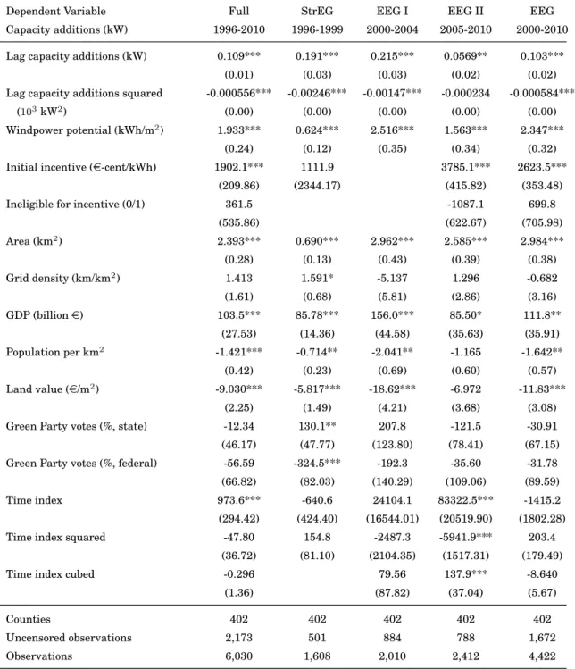
The regression results are robust across specifications. StrEG and EEG incentives, wind-power potential, lag capacity additions, county area, and GDP have a significantly positive effect on wind power development, while squared lag capacity additions, population density, and land value have a negative effect. A 1e-cent/kWh increase in the FIT would lead to an in-crease in capacity additions of around 1.9 MW per county per year over the entire 1996-2010 period. The effect would be even greater in 2005-2010 with capacity additions increasing by 3.8 MW per county in the 2005-2010 period. At the national level, this amounts to 764 MW per year for 1996-2010 and 1,528 MW per year for 2005-2010, calculated by multiplying with regression estimates by the 402 counties.
In all three Tables, access to the grid as measured by grid density emerges as an impor-tant determinant of wind power investment only during the StrEG from 1996-1999. The lack of significance in later years reflects the fact that new renewable power plants were guar-anteed access to the grid with grid operators paying for any necessary upgrade costs. The allocation of interconnection costs between plant developers and grid operators changed in 2000 with the EEG. While the StrEG did not specify how costs are allocated, the EEG shifted the majority of the costs (system upgrade costs) to grid operators. As expected, beginning in 2000 grid interconnection costs no longer figure into wind power developer’s location de-cisions. This system of shallow interconnection fees with essentially no location signal to developers has likely led to a distribution of wind power plants across Germany that makes suboptimal use of the existing grid infrastructure, requiring more grid upgrades than other-wise necessary. In the United States, renewable power plants are for the most part respon-sible for system upgrade costs, which acts as a location signal to developers. A similar study of wind power development in the United States finds that transmission line coverage has a significant positive effect on additions to wind power capacity [Hitaj, 2013].
Table 3 shows how the relative importance of windpower potential, the incentive level, and grid density changes over time. Grid density becomes less important beginning in 2000 while windpower potential and the level of the initial FIT become more important. This indicates that in later years, the EEG incentive becomes the main driver of wind power de-velopment. Table 4 confirms this result. The coefficient on discounted incentive revenue on capacity additions increases from 3.36 in 1996-1999 to 16.11 in 2000-2010, while the effect
of other variables, such as grid density or lag capacity additions declines. This result is ex-pected, since the “best” wind power locations are developed first. As time goes on, the remain-ing sites become less and less desirable, such that the relative importance of any incentive increases. However, this result also reflects the changing nature of the FIT in Germany from the uniform incentive during the StrEG to the wind-dependent design during the EEG. Un-der the EEG, wind power development is supported more heavily in less suitable (less windy) locations, such that the incentive gains, by design, greater relative importance during the EEG as compared with the StrEG.
As a robustness check, Table 5 shows the regression results using non-discounted incen-tive revenue to capture the EEG. Again, the coefficient on non-discounted incenincen-tive revenue on capacity additions increases from 1.78 in 1996-1999 to 8.57 in 2000-2010. The model is also estimated using ordinary least squares (Table 9 in the Appendix), yielding similar results.
It is difficult to measure the effect of ineligibility on wind capacity additions, since data are at the county level. Average wind levels within a county could signal ineligibility, while parts of the county remain eligible. The indicator variable, ineligible, measured with a less stringent 50% reference output cutoff, is not significant. However, the change in regulations in 2004 making less windy sites ineligible is not meaningless; ineligibility measured at 60% of reference output appears to capture “just” eligible counties, which has a significant posi-tive effect on capacity additions (Table 10). Ineligibility measured at 50% is conversely not significantly negative, since these counties may be undesirable in any case.13
Thus, the regulatory change that took place in 2004 marking less windy sites as ineli-gible for the incentive had a significant effect on capacity additions with wind power devel-opers taking advantage of available incentives up until the ineligibility cutoff. While such a measure is likely to reduce investment in windpower in locations with suboptimally low windpower potential, the design as a sharp cut-off point is not efficient as the net benefits of windpower plants do not drop from a large positive value to zero at some particular level of windpower potential. The decline is likely to be smooth, which an efficient incentive design would reflect.
From 1996-1999, the county-level share of Green Party votes in the state election has a positive impact on wind power development, suggesting that wind developers take local atti-tudes into account when siting turbines. Conversely, support for the Green party at the fed-eral level has a negative effect, probably because many non-environmentalists voted Green as a rejection of the ruling conservative party. This relationship flipped by 2005-2010. At this later stage, the EEG formed an important part of the national debate, and citizens recog-nized that subsidies were set by the federal government. Support for the Green party at the federal level thus has a positive effect on wind power development. The negative effect of the share of Green Party votes in state elections indicates that citizens may support wind power in general but resist development in their immediate surroundings (NIMBYism). As Green Party voters, these citizens presumably place a high premium on their local environment and may oppose the visual and auditory impacts of wind turbines on the local community.
13Of the 72 ineligible counties measured at a 50% cut-off, 30 counties experienced wind-power development by 2004. However, cumulative capacity in those counties in 2004 reached 162 MW, which is only 0.6% of the total installed capacity of 26,600 MW.
Table 3: Wind Power Capacity Tobit Marginal Effects - Initial Incentive
Dependent Variable Full StrEG EEG I EEG II EEG
Capacity additions (kW) 1996-2010 1996-1999 2000-2004 2005-2010 2000-2010
Lag capacity additions (kW) 0.109*** 0.191*** 0.215*** 0.0569** 0.103***
(0.01) (0.03) (0.03) (0.02) (0.02)
Lag capacity additions squared -0.000556*** -0.00246*** -0.00147*** -0.000234 -0.000584***
(103kW2) (0.00) (0.00) (0.00) (0.00) (0.00)
Windpower potential (kWh/m2) 1.933*** 0.624*** 2.516*** 1.563*** 2.347***
(0.24) (0.12) (0.35) (0.34) (0.32)
Initial incentive (e-cent/kWh) 1902.1*** 1111.9 3785.1*** 2623.5***
(209.86) (2344.17) (415.82) (353.48)
Ineligible for incentive (0/1) 361.5 -1087.1 699.8
(535.86) (622.67) (705.98) Area (km2) 2.393*** 0.690*** 2.962*** 2.585*** 2.984*** (0.28) (0.13) (0.43) (0.39) (0.38) Grid density (km/km2) 1.413 1.591* -5.137 1.296 -0.682 (1.61) (0.68) (5.81) (2.86) (3.16) GDP (billione) 103.5*** 85.78*** 156.0*** 85.50* 111.8** (27.53) (14.36) (44.58) (35.63) (35.91) Population per km2 -1.421*** -0.714** -2.041** -1.165 -1.642** (0.42) (0.23) (0.69) (0.60) (0.57) Land value (e/m2) -9.030*** -5.817*** -18.62*** -6.972 -11.83*** (2.25) (1.49) (4.21) (3.68) (3.08)
Green Party votes (%, state) -12.34 130.1** 207.8 -121.5 -30.91
(46.17) (47.77) (123.80) (78.41) (67.15)
Green Party votes (%, federal) -56.59 -324.5*** -192.3 -35.60 -31.78
(66.82) (82.03) (140.29) (109.06) (89.59)
Time index 973.6*** -640.6 24104.1 83322.5*** -1415.2
(294.42) (424.40) (16544.01) (20519.90) (1802.28)
Time index squared -47.80 154.8 -2487.3 -5941.9*** 203.4
(36.72) (81.10) (2104.35) (1517.31) (179.49)
Time index cubed -0.296 79.56 137.9*** -8.640
(1.36) (87.82) (37.04) (5.67)
Counties 402 402 402 402 402
Uncensored observations 2,173 501 884 788 1,672
Observations 6,030 1,608 2,010 2,412 4,422
Table 4: Wind Power Capacity Tobit Marginal Effects - Incentive Revenue
Dependent Variable Full StrEG EEG I EEG II EEG
Capacity additions (kW) 1996-2010 1996-1999 2000-2004 2005-2010 2000-2010
Lag capacity additions (kW) 0.111*** 0.192*** 0.214*** 0.0311 0.0937***
(0.01) (0.03) (0.03) (0.02) (0.02)
Lag capacity additions squared -0.000533*** -0.00247*** -0.00144*** -0.0000501 -0.000509**
(103kW2) (0.00) (0.00) (0.00) (0.00) (0.00)
Incentive revenue 12.71*** 3.361*** 14.09*** 14.25*** 16.11***
(e/m2, 7% discount) (1.35) (0.65) (2.04) (2.38) (1.92)
Ineligible for incentive (0/1) 248.4 -435.4 773.5
(527.16) (788.14) (722.96) Area (km2) 2.435*** 0.689*** 2.960*** 2.919*** 3.095*** (0.29) (0.13) (0.43) (0.43) (0.39) Grid density (km/km2) 1.345 1.589* -5.235 1.080 -0.777 (1.64) (0.68) (5.83) (3.10) (3.30) GDP (billione) 89.81** 85.86*** 153.5*** 69.43 97.60** (27.96) (14.35) (44.87) (38.84) (37.10) Population per km2 -1.467*** -0.715** -2.047** -1.238 -1.705** (0.43) (0.23) (0.69) (0.65) (0.59) Land value (e/m2) -8.674*** -5.856*** -18.43*** -8.799* -11.40*** (2.28) (1.49) (4.24) (3.96) (3.16)
Green Party votes (%, state) -72.41 131.2** 212.8 -245.1** -74.02
(45.83) (47.73) (123.99) (82.31) (67.68)
Green Party votes (%, federal) 85.41 -325.5*** -194.5 250.5* 90.26
(63.93) (81.98) (140.61) (110.71) (87.99)
Time index 1845.7*** 546.8 24081.2 27573.2 3648.2*
(271.77) (3028.33) (16528.32) (19978.93) (1515.00)
Time index squared -164.6*** -212.7 -2485.1 -2070.1 -344.1*
(32.67) (907.27) (2102.36) (1490.19) (144.55)
Time index cubed 4.164*** 32.84 79.50 50.69 9.625*
(1.19) (86.02) (87.73) (36.73) (4.41)
Counties 402 402 402 402 402
Uncensored observations 2,173 501 884 788 1,672
Observations 6,030 1,608 2,010 2,412 4,422
Table 5: Wind Power Capacity Tobit Marginal Effects - Undiscounted
Incen-tive Revenue
Dependent Variable: Full StrEG EEG I EEG II EEG
Capacity additions (kW) 1996-2010 1996-1999 2000-2004 2005-2010 2000-2010
Lag capacity additions (kW) 0.111*** 0.192*** 0.214*** 0.0313 0.0936***
(0.01) (0.03) (0.03) (0.02) (0.02)
Lag capacity additions squared -0.000527*** -0.00247*** -0.00144*** -0.0000452 -0.000504**
(103kW2) (0.00) (0.00) (0.00) (0.00) (0.00)
Incentive revenue 6.558*** 1.780*** 7.610*** 7.538*** 8.572***
(e/m2, 0% discount) (0.71) (0.35) (1.11) (1.30) (1.04)
Ineligible for incentive (0/1) 207.5 -458.9 763.3
(522.52) (791.47) (722.87) Area (km2) 2.448*** 0.689*** 2.953*** 2.929*** 3.102*** (0.29) (0.13) (0.43) (0.43) (0.39) Grid density (km/km2) 1.321 1.589* -5.256 1.066 -0.790 (1.64) (0.68) (5.83) (3.11) (3.31) GDP (billione) 89.14** 85.86*** 152.6*** 68.56 96.65** (27.96) (14.35) (44.92) (38.95) (37.19) Population per km2 -1.470*** -0.715** -2.050** -1.244 -1.711** (0.43) (0.23) (0.69) (0.65) (0.59) Land value (e/m2) -8.905*** -5.856*** -18.38*** -8.996* -11.51*** (2.28) (1.49) (4.25) (3.97) (3.16)
Green Party votes (%, state) -72.90 131.2** 214.1 -244.7** -73.10
(45.86) (47.73) (124.00) (82.47) (67.73)
Green Party votes (%, federal) 92.82 -325.5*** -194.5 259.1* 95.31
(63.93) (81.98) (140.64) (110.86) (88.05)
Time index 1866.3*** 546.8 24091.9 27496.8 3608.3*
(272.31) (3028.33) (16525.52) (20018.77) (1518.53)
Time index squared -166.9*** -212.7 -2487.0 -2064.1 -340.2*
(32.72) (907.27) (2102.01) (1493.04) (144.94)
Time index cubed 4.247*** 32.84 79.60 50.53 9.507*
(1.19) (86.02) (87.72) (36.80) (4.42)
Counties 402 402 402 402 402
Uncensored observations 2,173 501 884 788 1,672
Observations 6,030 1,608 2,010 2,412 4,422
* p<0.10, ** p<0.05, *** p<0.01, standard errors in parentheses
5.1 Analysis of Counterfactual Scenarios: Uniform Incentives
In this section we explore the effect of a uniform incentive on wind power development across counties. Beginning with the EEG in 2000, the federal incentive for wind power varied according to wind power potential with less windy sites receiving a higher FIT rate than more windy sites. This translates into incentive revenue increasing linearly with windpower potential but then gradually flattening out until the maximum incentive is reached. Here, we estimate capacity additions over time under a different hypothetical FIT regime - a uniform national incentive that does not vary with wind power potential.
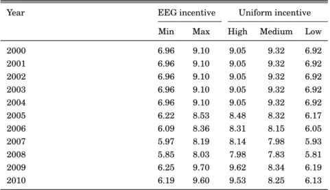
Three different hypothetical FIT levels are considered (Table 6). In all three cases, all lo-cations are presumed eligible to receive the incentive, in contrast to the EEG, which excludes locations with output less than 60% of reference output after August 1, 2004.14 Under the EEG, the 5-year period with the higher initial incentive is extended depending on the loca-tion’s windiness, such that the 20-year average FIT varies across counties. The high, medium and low counterfactual incentives are calculated as follows (Table 6). The low FIT is equiva-lent to the 20 year average of the minimum FIT achieved under the EEG, namely 5 years of the initial FIT and 15 years of the base FIT. The high FIT is calculated as the average across counties of the realized 20-year-average EEG FIT. The medium FIT equals about 1.35 times the low FIT. Its level is chosen such that the total predicted installed capacity under the EEG and the medium FIT are equal to allow for better comparison. We also include the case when no FIT subsidies are offered.
Table 6: Hypothetical Average Feed-In Tariffs (
e
-cent/kWh)
Year EEG incentive Uniform incentive
Min Max High Medium Low
2000 6.96 9.10 9.05 9.32 6.92 2001 6.96 9.10 9.05 9.32 6.92 2002 6.96 9.10 9.05 9.32 6.92 2003 6.96 9.10 9.05 9.32 6.92 2004 6.96 9.10 9.05 9.32 6.92 2005 6.22 8.53 8.48 8.32 6.17 2006 6.09 8.36 8.31 8.15 6.05 2007 5.97 8.19 8.14 7.98 5.93 2008 5.85 8.03 7.98 7.83 5.81 2009 6.25 9.70 9.62 8.34 6.19 2010 6.19 9.60 9.53 8.25 6.13
A priori, it is unclear whether the uniform incentive or the wind-dependent EEG incentive achieves greater wind power output per euro (kWh/e). Presumably, the EEG will achieve lower wind power output per installed turbine, since it offers a reduced incentive in very windy areas. However, the uniform incentive may overspend on subsidies for wind turbines in high-wind areas, which would experience development even at lower incentive levels. Thus, while the uniform incentive is expected to outperform the EEG in terms of wind power output per installed turbine, the relative standings in terms of wind power output per euro are unclear.
The impact of the incentive structure on emission reductions per euro (CO2 kg/e) is also uncertain. This depends in part on how well the different incentive structures perform in terms on kWh/e. However, it also depends on the degree of correlation between windiness and regional emissions. If windiness and regional emissions are negatively correlated net of other factors that affect a location’s suitability, the EEG could achieve greater reductions in emissions per euro spent than a uniform incentive.
14In our county-level annual analysis, those locations are captured as counties with poten-tial output less than 50% of reference output after December 31, 2004.
Annual additions to installed capacity are predicted under the EEG as well as the high, medium, and low uniform incentives. Since the level of the uniform incentives are contained within the bounds of actual EEG incentive levels experienced across counties, the prediction can be considered in-sample. It is of course expected that predicted and actual capacity addi-tions under the EEG diverge to some extent. Indeed, the EEG prediction using actual EEG capacity for the lag capacity variable does well. Actual EEG installed capacity and output reaches 23.34 GW and 229.5 TWh, while we predict 21.63 GW and 217.2 TWh.
However, we must focus on the case where predicted capacities are used as lag capacities in the following year to avoid biasing the predicted distribution towards the actual distribu-tion. As 10 years of capacity additions are predicted in this way, errors compound and the predicted EEG capacity additions diverge quite substantially from actual capacity additions towards 2010. With this prediction method, total predicted capacity reaches 8.806 GW com-pared to the actual capacity of 23.34 GW. However, we are more interested in comparing pre-dicted capacity additions across the different incentive structures than in the absolute level of predicted capacity additions. The divergence between predicted and actual EEG capacity additions is therefore less of an issue.
Table 7 presents the results of the counterfactual analysis, showing the total cost, in-stalled capacity, expected wind power output, and avoided carbon dioxide emissions for each of the scenarios considered. In addition, measures of efficiency are computed, including out-put per euro spent (kWh/e) and avoided emissions per euro spent (CO2 kg/e). We estimate
that about 0.538 GW or 6% of predicted capacity would have been installed even if there had been no FIT incentive, mainly in northern Germany. The uniform low incentive achieves the greatest wind power output and CO2emission reductions per euro spent at 15.38 kWh/eand
4.658 kg/e. This result is not surprising. Higher levels of efficiency are of course achieved at lower total levels of wind power development, as prime locations are developed before less suitable locations.
The medium incentive can be more directly compared with the EEG prediction. The in-centive level is set at about 1.35 times the low inin-centive such that the total installed capacity under the medium uniform incentive matches that of the EEG prediction at 8.806 GW. For the same amount of installed capacity, wind power output under the EEG (86.65 TWh) is lower than under the uniform incentive (88.93TWh). However, at 7.828 billion euros, the uniform incentive is more costly than the EEG at 7.554 billion euros, since the EEG reduces costs by recognizing that windy areas require less support to make an attractive investment. Overall, the EEG performs slightly better than the equivalent uniform incentive in terms of output per euro (11.47 kWh/ecompared with 11.36 kWh/e) and emission reductions per euro (3.596 kg/ecompared with 3.469 kg/e). However, the improvement is marginal at 1% for output per euro and 3.7% for emission reductions per euro.
The EEG would likely perform even better than a uniform incentive if transmission con-gestion were taken into account. High concentrations of wind power in particular areas and transmission constraints mean that not all of the wind power can be transported to electricity demand areas. Compared with a uniform incentive, the EEG results in a more distributed arrangement of wind power plants across the transmission grid and thus lower levels of con-gestion and higher levels of emission reductions. The 3.7% improvement over a uniform incentive in terms of emission reductions per euro would likely increase if transmission con-gestion is considered.
Table 7: Relative Efficiency of the EEG and Uniform Incentives
Scenario Capacity Output Cost Avoided CO2 Efficiency
emissions Output Abatement
(GW) (TWh) (billion /e) (million ton) (kWh/e)* (CO2kg/e)*
Predicted EEG 8.806 86.65 7.554 27.17 11.47 3.596
Medium incentive 8.806 88.93 7.828 27.16 11.36 3.469
High incentive 9.105 92.13 8.218 28.14 11.21 3.425
Low incentive 4.972 49.80 3.255 14.92 15.30 4.584
No incentive 0.538 5.045 0 1.416
The cost and efficiency measures are undiscounted values. Due to the time value of money, a better estimate of EEG cost would involve discounting, which could not be implemented in this calibration exercise. Thus, it is appropriate to compare the relative efficiency of the different policy scenarios presented in this paper, but it does not make sense to compare the amount of avoided carbon emissions per euro with other abatement technologies. These values do, however, give an upper bound, since discounting would only lower the cost. The high incentive is the county-average EEG incentive by year, while the low incentive assumes the lowest possible EEG incentive (5 years higher initial incentive and 15 years lower base incentive). The medium incentive is about 1.35 times the low incentive.
The counterfactual analysis demonstrates that a uniform incentive would have resulted in a different distribution of wind power plants across counties. Graph 5 shows the difference in predicted cumulative capacity in 2010 between the EEG and uniform medium incentive. Under the uniform incentive, significantly more development occurs in the northern coastal counties with the greatest wind power potential (marked as white in the graph). The wind-dependent incentive of the EEG leads to relatively greater development in all other counties (shaded blue), thus resulting in a more distributed arrangement of wind power plants across Germany. However, the differences in installed capacities in non-Northern counties between the two types of incentives is relatively small.
[8,1638] (1638,4461] (4461,6399] (6399,7974] (7974,11772] (11772,21545] (21545,50464] Differences in Cumulative Capacity (EEG - Medium) 2010
Figure 5: Differences in Predicted Cumulative Capacity (kW) in 2010 (EEG
-Medium Incentive)
∗∗More wind power capacity is installed in the northern coastal counties under the uniform medium incentive than
under the EEG, as indicated by the white color. All other counties (shaded blue) experience greater wind power development under the EEG.