A Dissertation by
NAI-WEI CHEN
Submitted to the Office of Graduate Studies of Texas A&M University
in partial fulfillment of the requirements for the degree of DOCTOR OF PHILOSOPHY
December 2011
A Dissertation by
NAI-WEI CHEN
Submitted to the Office of Graduate Studies of Texas A&M University
in partial fulfillment of the requirements for the degree of DOCTOR OF PHILOSOPHY
Approved by:
Chair of Committee, Thomas E. Wehrly Committee Members, Jeffrey D. Hart
Dominique Lord Simon Sheather Head of Department, Simon Sheather
December 2011 Major Subject: Statistics
ABSTRACT
Goodness-of-Fit Test Issues in Generalized Linear Mixed Models. (December 2011)
Nai-Wei Chen, B.B.A., Tunghai University; M.S., National Central University
Chair of Advisory Committee: Dr. Thomas E. Wehrly
Linear mixed models and generalized linear mixed models are random-effects models widely applied to analyze clustered or hierarchical data. Generally, random effects are often assumed to be normally distributed in the context of mixed mod-els. However, in the mixed-effects logistic model, the violation of the assumption of normally distributed random effects may result in inconsistency for estimates of some fixed effects and the variance component of random effects when the variance of the random-effects distribution is large. On the other hand, summary statistics used for assessing goodness of fit in the ordinary logistic regression models may not be directly applicable to the mixed-effects logistic models. In this dissertation, we present our investigations of two independent studies related to goodness-of-fit tests in generalized linear mixed models.
First, we consider a semi-nonparametric density representation for the random-effects distribution and provide a formal statistical test for testing normality of the random-effects distribution in the mixed-effects logistic models. We obtain estimates of parameters by using a non-likelihood-based estimation procedure. Additionally, we not only evaluate the type I error rate of the proposed test statistic through asymptotic results, but also carry out a bootstrap hypothesis testing procedure to
control the inflation of the type I error rate and to study the power performance of the proposed test statistic. Further, the methodology is illustrated by revisiting a case study in mental health.
Second, to improve assessment of the model fit in the mixed-effects logistic mod-els, we apply the nonparametric local polynomial smoothed residuals over within-cluster continuous covariates to the unweighted sum of squares statistic for assessing the goodness-of-fit of the logistic multilevel models. We perform a simulation study to evaluate the type I error rate and the power performance for detecting a missing quadratic or interaction term of fixed effects using the kernel smoothed unweighted sum of squares statistic based on the local polynomial smoothed residuals over x-space. We also use a real data set in clinical trials to illustrate this application.
ACKNOWLEDGMENTS
I have tremendous appreciation for my advisor Dr. Thomas E. Wehrly. Finite words cannot express how blessed I am in my life. I thank him for his patient guidance, trust, and encouragement on the pursuit of my Ph.D. degree. I not only gained confidence to explore and develop my statistical ideas through his inspiration, but also learned a lot for future development through our talks. I will bear whatever he instructed in mind forever.
I also sincerely thank Dr. Jeffrey D. Hart for his generous support and advice throughout my research. Along with Dr. Hart, I would like to express my appreciation to Dr. Simon Sheather and Dr. Dominique Lord for their support as members of my advisory committee. Additionally, I particularly thank Dr. Michael Longnecker for offering me financial support during the final term of my graduate studies.
Moreover, I offer special thanks to my colleagues, Junbum Lee, Ganggang Xu, and Paul Martin, for their friendship. Finally, I extend a sincere thanks to my spiritual family. I am grateful to my parents and my sisters for their love and encouragement. Without their firm support, I could not accomplish the goal and complete this amazing journey.
TABLE OF CONTENTS
CHAPTER Page
I INTRODUCTION. . . 1
II LITERATURE REVIEW . . . 6
2.1 Generalized Linear Mixed Models . . . 6
2.2 Estimation Procedure . . . 7
2.2.1 Parameter Estimation in the Conditional Case . . . . 9
2.2.2 Parameter Estimation in the Marginal Case . . . 10
2.3 Application of Smoothed Residuals in the Ordinary Lo-gistic Models . . . 12
III A TEST FOR NORMALITY OF RANDOM EFFECTS IN GENERALIZED LINEAR MIXED MODELS . . . 15
3.1 Introduction . . . 15
3.2 Robust Score Test Statistic with Estimating Equations . . . 17
3.3 A Test of Normality of Random Effects in GLMMs . . . 21
3.3.1 SNP Density Representation of the Random-Effects Distribution . . . 21
3.3.2 Implementation of the Test for Normality of Ran-dom Effects . . . 22
3.3.3 Bootstrap Hypothesis Testing . . . 27
3.4 Simulation Study . . . 29
3.4.1 Type I Error Rate via Asymptotic Results . . . 29
3.4.2 Type I Error Rate via Smoothed Bootstrap Test . . . 31
3.4.3 Power Analysis via Smoothed Bootstrap Test . . . 33
3.5 Application . . . 36
3.6 Discussion . . . 44
IV LOCAL POLYNOMIAL SMOOTHED RESIDUALS APPLIED TO ASSESS THE LOGISTIC MULTILEVEL MODEL . . . 46
4.1 Introduction . . . 46
4.2 Goodness-of-fit Tests for the Logistic Multilevel Models . . 47
4.2.1 Multilevel Models for Binary Data . . . 47
4.2.2 Goodness-of-Fit Test Statistic . . . 49
CHAPTER Page
4.3 Simulation Study . . . 54
4.3.1 Type I Error Rate for the Random Intercept Model . 55 4.3.2 Power Analysis for the Random Intercept Model . . . 60
4.3.3 Power Analysis for the Random Intercept and Slope Model . . . 64 4.4 Application . . . 68 4.5 Discussion . . . 73 V CONCLUSION . . . 75 REFERENCES . . . 79 APPENDIX A . . . 85 APPENDIX B . . . 87 VITA . . . 91
LIST OF TABLES
TABLE Page
1 Results of the type I error rate using the asymptotic distribution
of TRS,m for three cluster sizes whenσ2=16, 32, 48 and 64. . . 30 2 Results of the type I error rate using the smoothed bootstrap test
procedure with bootstrap sample size B=60 for cluster size n=5
and tij=(−0.1,0,0.1,0.2,0.3) when σ2=16, 32 and 64.. . . 32 3 Results of the type I error rate using the smoothed bootstrap test
procedure with bootstrap sample size B=60 for cluster size n=6
and tij=(0,1,2,4,6,8) when σ2=16 and 32. . . 33 4 Results of the type I error rate using the smoothed bootstrap test
procedure with bootstrap sample sizeB=100 for cluster size n=6
and tij=(0,1,2,4,6,8) when σ2=16 and 32. . . 33 5 Results of the power performance of bimodal and multimodal
al-ternatives using the smoothed bootstrap test procedure with boot-strap sample sizeB=60 for cluster sizen=6 andtij=(0,1,2,4,6,8)
when σ2=16 and 32. . . 34 6 Results of the power performance of skewed and heavy-tailed
al-ternatives using the smoothed bootstrap test procedure with boot-strap sample sizeB=60 for cluster sizen=6 andtij=(0,1,2,4,6,8)
when σ2=16 and 32. . . . . 35
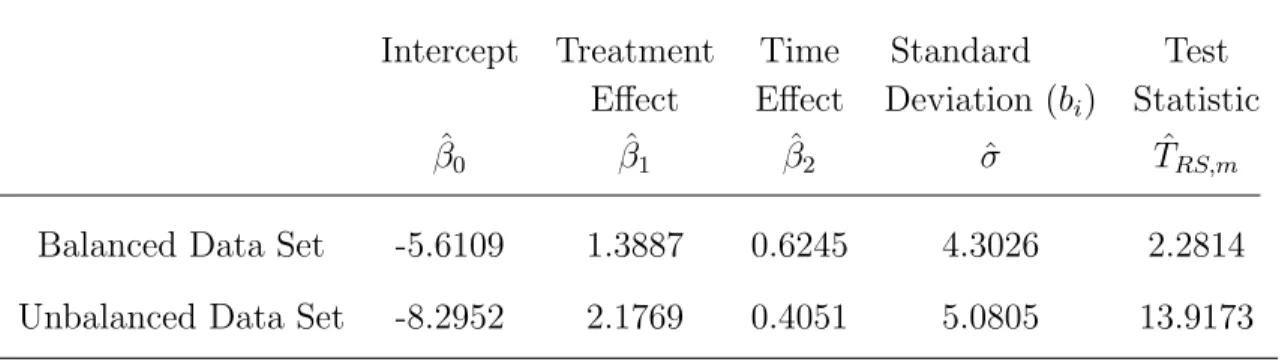
7 Estimates of parameters under IEE procedure and the proposed test statistic value, ˆTRS,m, on testing normality of random effects
for balanced and unbalanced data sets in mental health study. . . 38 8 Mean and standard deviation (S.D.) of bootstrap parameter
esti-mates with bootstrap sample size B=50, 100, 200, 300, 400 and
500 for the balanced data set in mental health study. . . 39 9 Mean and standard deviation (S.D.) of bootstrap parameter
esti-mates with bootstrap sample size B=50, 100, 200, 300, 400 and
TABLE Page 10 Results of normality test of the distribution of random effects
under the smoothed bootstrap procedure in mental health study. . . 43 11 Comparisons of the type I error rate for three types of asymptotic
distributions of the kernel smoothed unweighted sum of squares
statistic by smoothing residuals in the y-space. . . 57 12 P-values of normality checking of Case 1 for (1)ZSm and (2)cSmtran.. . 58 13 Results of the type I error rate of Sm by using local polynomial
smoothed residuals are computed based on the scaled chi-squared
distributioncSm. . . 59 14 Results of the power performance of detecting a missing strong or
moderate within-cluster quadratic term of fixed effects when the
alternative model (4.4) is assumed. . . 62 15 Results of the power performance of detecting a missing strong
within-cluster interaction term of fixed effects between Bernoulli
and continuous covariates when the alternative model (4.5) is assumed. 63 16 Results of the power performance of detecting a missing strong
within-cluster interaction term of fixed effects between two
con-tinuous covariates when the alternative model (4.6) is assumed. . . . 64 17 Results of controlling type I error rate ofSm by using local
poly-nomial smoothed residuals are computed based oncSm when the
model includes random intercept and slope. . . 66 18 Results of the power performance of detecting a missing strong or
moderate within-cluster quadratic term of fixed effects when the
alternative model (4.7) with random intercept and slope is assumed. 67 19 List of six logistic multilevel models with the random intercept
for demonstrating the application. . . 69 20 Results of the selected values of smoothing parameter based on
TABLE Page 21 Results of the model fit based on glmmPQL and glmer and model
checking based onSm by using local polynomial smoothing resid-uals over within continuous cluster-level covariates for Model 1,
Model 2 and Model 3. . . 71 22 Results of the model fit based on glmmPQL and glmer and model
checking based onSm by using local polynomial smoothing resid-uals over within continuous cluster-level covariates for Model 4,
Model 5 and Model 6. . . 72 23 P-values of normality checking of Case 2 to Case 4 for (1)ZSm and
(2)cStran
LIST OF FIGURES
FIGURE Page
1 The distribution of empirical Bayes estimates of random effects based on the specified model (3.5) for balanced and unbalanced
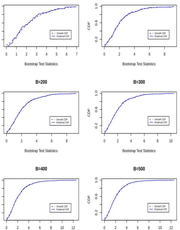
data sets in mental health study. . . 37 2 Empirical and kernel estimates of a distribution function for
boot-strap test statistics with bootboot-strap sample size B = 50, 100, 200, 300, 400 and 500 in the analysis of the balanced data set in mental
health study. . . 41 3 Empirical and kernel estimates of a distribution function for
boot-strap test statistics with bootboot-strap sample size B = 50, 100, 200, 300, 400 and 500 in the analysis of the unbalanced data set in
mental health study. . . 42 4 Normal QQ plots of test statistic values of Case 1 under (1)ZSm
and (2)cStran
m : the smoothed residuals over y-space based on
1 4
√
N
and 12√N are shown on the top and bottom panels, respectively.. . . 58 5 Normal QQ plots of test statistic values of Case 2 under (1)ZSm
and (2)cStran
m : the smoothing residuals over y-space based on
1 4
√
N and 12√N are demonstrated on the top and bottom
pan-els, respectively. . . 88 6 Normal QQ plots of test statistic values of Case 3 under (1)ZSm
and (2)cSmtran: the smoothing residuals over y-space based on
1 4 √ N and 1 2 √
N are demonstrated on the top and bottom
pan-els, respectively. . . 89 7 Normal QQ plots of test statistic values of Case 4 under (1)ZSm
and (2)cSmtran: the smoothing residuals over y-space based on
1 4
√
N and 12√N are demonstrated on the top and bottom
CHAPTER I
INTRODUCTION
In most data analysis, linear models (LMs) have been widely used in cases where the observed outcome variables are continuous. When the observed outcome variables are categorical or discrete, generalized linear models (GLMs) possessing nonnormal out-come distributions and their mean functions (McCullagh and Nelder, 1989; Agresti, 2002) play an important role. Additionally, in practice, clustered or hierarchical data often occur in many fields, for instance, in the biomedical field where repeated mea-surements are taken over time on each of many subjects in a sample or in the field of education where we can group students by the district and measurements are taken on students within districts. On the above examples, outcome variables are usu-ally correlated because repeated measurements are made on each subject or subjects within clusters may exhibit similar characteristics. Therefore, LMs and GLMs are not applicable in accounting for this dependence.
In the past decade, models including a vector of unobserved subject-specific ef-fects, namely random efef-fects, in the linear predictor component of the model are used to deal with multiple sources of variation. In random-effects models, it is of-ten assumed that conditional on the random effects, the observed outcomes within each subject or cluster are independent and random parts can be between subjects or within subjects. Nowadays, linear mixed models (LMMs) and generalized linear mixed models (GLMMs) are random-effects models used to model normal and non-normal observed outcomes, respectively. They have been widely applied in many different fields such as epidemiological studies of diseases, toxicology, and so on (Ver-The format follows the style of Journal of the American Statistical Association.
beke and Molenberghs, 2000; Diggle et al., 2002; Molenberghs and Verbeke, 2005). Undoubtedly, in the context of mixed models, estimation and inference depend that the structure of random effects is correctly specified. In general, random effects are unobserved and in most inferential procedures and computation implementation, random effects are often assumed to be normally distributed in LMMs and GLMMs. In LMMs, Verbeke and Lesaffre (1997) showed that maximum likelihood estima-tors (MLEs) for fixed effects and variance components of random effects obtained under the assumption of normally distributed random effects are consistent, even when the random-effects distribution is misspecified. Unlike LMMs some research has been done to discover the impact of misspecifying the random-effects distribution in the mixed-effects logistic model, a broadly discussed case with binary outcomes in GLMMs.
Neuhaus et al. (1992) carried out a set of simulation studies to find that when the distribution of random effects is misspecified and a random-intercept logistic model is fitted, the MLEs of model parameters for the fixed effects are inconsistent, but the magnitude of the bias is not large. However, estimates of the variance of the random-effects distribution exhibit large biases. Heagerty and Kurland (2001) used the Kullback-Leibler Information Criterion to evaluate the consistency of MLEs of model parameters on conditional and marginal mean models. The authors showed that for conditionally specified models, misspecification of the random-effects distri-bution may lead to seriously biased estimators for a cluster-level (between-subject) parameter and the intercept term when the variance of the random-effects distri-bution is large. Agresti et al. (2004) showed that the MLEs for fixed effect and variance component of the random-effects distribution appear inconsistent when the true random-effects distribution is a two-points mixture with a large variance in a simple one-way random-effects model. Liti`ere et al. (2008), through simulations,
found that MLEs of between-subject parameters for the mean structure may be af-fected by misspecification of the random-effects distribution when the variance of the true random-effects distribution is large and estimates of the variance component are severely affected by misspecification in most situations.
Moreover, Liti`ere et al. (2007) studied the impact of the misspecification of the random-effects distribution on the type I and type II error rates related to the Wald test for the mean structure parameters. They found that misspecification of the random-effects distribution and the variance component of random effects can severely affect the power of the analysis and the type I error rate related to the tests for the intercept parameter. Huang (2009) proposed a novel two-step parametric diagnostic method that makes use of both observed data and a reconstructed data set induced from the observed data to verify misspecification of the random-effects model. In terms of one of the simulation results, the author showed that when the distribution family of random effects is misspecified, the test for the corresponding variance component of the random-effects distribution tends to be significant but the proposed test statistic loses power on testing the parameters of fixed effects. Therefore, an assessment of the goodness of fit of the random-effects distribution increasingly becomes a study issue in generalized linear mixed models.
On the other hand, since the mixed-effects logistic models have been widely used for analyzing clustered or naturally hierarchical data with binary outcomes, methods for assessment of the model fit need to be well developed. Evans and Hosmer (2004) extended summary statistics used on assessing goodness of fit in the ordinary logistic regression models to mixed-effects logistic models. The authors showed that the performance of type I error rates is not good in some situations. Additionally, Sturdivant (2005) and Sturdivant and Hosmer (2007) proposed a kernel smoothed unweighted sum of squares statistic by smoothing residuals in the y-space to assess the
adequacy of the logistic multilevel models. They demonstrated satisfactory adherence to type I error rates by the proposed statistic. However, for a case with fewer subjects per cluster, the simulation results showed very limited or no power to detect the missing quadratic term of fixed effects. Therefore, finding a method for improving the existing methods of assessment of the model fit in any specified model is worth being discussed.
The objective of this dissertation includes two independent studies in mixed-effects logistic models. The first work is to provide a method for testing normality of the random-effects distribution and the second work is to apply the nonparamet-ric local polynomial smoothed residuals to improve assessment of the model fit. In Chapter II, we present a literature review for our two studies. Chapter III of this dissertation is devoted to our first study. We consider a semi-nonparametric (SNP) density representation for the random-effects distribution and provide a formal sta-tistical test that has a close connection to an order selection-type goodness-of-fit test for testing normality of the random-effects distribution in GLMMs. This test is non-parametric in the sense that we do not assume a non-parametric form for the alternative model. In addition, estimation is fundamental to any hypothesis test. Unlike LMMs the likelihood function under GLMMs may have no analytic expression and numerical approximations may be needed. As a result, likelihood-based inference is computa-tionally challenging and non-likelihood-based estimation is an attractive approach. Zeger et al. (1988) used the generalized estimating equations (GEEs) approach to fit subject-specific and population-averaged models. Jiang (2007) and Jiang et al. (2007) proposed a procedure to solve estimating equations for parameter estimation. Throughout this study, a non-likelihood-based estimation procedure will be adopted for estimation of parameters. In a set of simulation studies, we conduct a bootstrap hypothesis testing procedure to evaluate the power performance and the type I error
rate for the proposed test statistic. Further, we apply our method to revisit a case study in mental health (Alonso et al., 2004; 2008).
Chapter IV is devoted to our second study. We apply the nonparametric lo-cal polynomial smoothed residuals over within-cluster continuous covariates to the unweighted sum of squares statistic (Hosmer et al., 1997; Sturdivant and Hosmer, 2007) for assessing the goodness-of-fit of the logistic multilevel models, namely, the mixed-effects logistic models for hierarchical data with binary outcomes. We carry out a simulation study which is performed to evaluate the type I error rate of the kernel smoothed unweighted sum of squares statistic by using the local polynomial smoothed residuals and the power performance for detecting a missing quadratic or interaction term of fixed effects. Moreover, to illustrate this application, we use a real data set in clinical trials provided by Cancer Biostatistics Center, Vanderbilt University. Finally, Chapter V recapitulates all our findings and provides discussions of future research.
CHAPTER II
LITERATURE REVIEW
In this chapter, we shall introduce the basic formulation of generalized linear mixed models and review some selected articles on parameter estimation in detail. Addition-ally, in this dissertation, one of our studies is related to an application of smoothed residuals in the logistic multilevel model for model checking. Therefore, we also in-troduce the original idea through reviewing an application of the smoothed residuals in the goodness-of-fit test of the ordinary logistic regression model.
2.1 Generalized Linear Mixed Models
Suppose there are m observed subjects (or clusters). Let us denote by yij the jth response measured, for instance, the jth time point in longitudinal data, for the ith subject (or cluster), i = 1, . . . , m and j = 1, . . . , ni. Further, for subject i, condi-tional on random effectsbi, all the responses yij are assumed to be independent with conditional density belonging to the exponential family (Molenberghs and Verbeke, 2005; Liti`ere et al., 2007),
f(yij|bi;β, φ) = exp yijθij −ψ(θij) φ +c(yij, φ) ,
whereψ(·) is a function satisfying E(yij|bi) =ψ0(θij), V ar(yij|bi) =φψ00(θij), and φ is a dispersion parameter whose value may be known andc(·,·) is a known function. Letµb
ij =E(yij|bi) =ψ0(θij). A generalized linear mixed model for yij is given by g(µbij) = g(E[yij|bi]) = xTijβ+z
T ijbi,
where g(·) is a monotonically increasing link function depending on known xij and
zij p-dimensional and q-dimensional vectors of fixed covariate values, including the intercept term;β, ap-dimensional vector of unknown fixed regression coefficients and
bi, a q-dimensional vector of the random effects. The subject-specific effects bi are generally assumed to be normally distributed with mean zero vector and variance-covariance matrix D, denoted byf(bi|D)∼N(0, D).
In clustered or hierarchical data analysis, the mixed-effects logistic models are often used to analyze binary outcome data collected in subjects (or clusters). Herein, we illustrate a special and important mixed-effects logistic model as follows.
Example 1. (Random-Intercept Logistic Model) Suppose the intercept terms bi are independent and identically distributed random effects. Within the ith subject (or cluster), binary responses yij are conditionally independent Bernoulli with
logit(µbij) =bi+xTijβ, whereµb
ij =p(yij = 1|bi,xij) and the dispersion parameterφ is assumed to be 1. This is a common case of generalized linear mixed models where the conditional exponential family is Bernoulli, bi is normally distributed with mean zero and variance σ2, and the link function is the logit-link, namely, the random-intercept logistic model.
2.2 Estimation Procedure
Generally, a random-effects model can be fitted by maximizing the marginal likeli-hood. The likelihood function is derived as
L(β, D, φ) = m Y i=1 Z ni Y j=1 f(yij|bi,β, φ)f(bi|D)dbi = m Y i=1 fi(yi|β, D, φ),
where yi = (yi1, . . . , yini)T. The likelihood function under GLMMs may have no ana-lytic expression and it cannot be further simplified. Thus, numerical approximations may be needed. As a result, likelihood-based inference in GLMMs is computationally challenging.
So far, several approaches about the inference of GLMMs have been developed. Based on Bayesian techniques, Zeger and Karim (1991) used Gibbs sampling tech-niques to take repeated samples from the posterior distributions to avoid the need of numerical integration, and Booth and Hobert (1999) used Monte Carlo EM algorithm for maximum likelihood estimation. Moreover, Breslow and Clayton (1993) proposed not only approximation of the marginal quasi-likelihood using the Laplace method which leads to estimating equations based the penalized quasi-likelihood for mean parameters in the marginal model, but also a penalized quasi-likelihood for approxi-mated inference on mean parameters and realizations of random effects in the condi-tional model. Lin and Breslow (1996) further developed first-order and second-order correction procedures for parameter estimation under the penalized quasi-likelihood. On the other hand, some computational methods based on the non-likelihood view-point are attractive. Zeger et al. (1988) used the generalized estimating equations (GEEs) approach to fit subject-specific and population-averaged models. Jiang (2007) and Jiang et al. (2007) proposed an iterative procedure to solve estimating equations for parameter estimation. In this section, we review two methods of parameter es-timation for generalized linear mixed models in detail. One excerpted from Breslow and Clayton (1993) is an approximation of the quasi-likelihood function in the con-ditional case; the other one excerpted from Jiang (2007) is an iterative procedure for solving estimating equations in the marginal case.
2.2.1 Parameter Estimation in the Conditional Case
When the exact likelihood function is difficult to compute, Breslow and Clayton (1993) applied the Laplace method for integral approximation to a quasi-likelihood function and modified the Fisher scoring algorithm developed by Green (1987) for parameter estimation. This method has been implemented in several statistical pack-ages.
Herein, we simplify the situation to a specified subject withnresponse measures. Suppose that, given a q-dimensional vector b of random effects, the responses y = (y1,· · · , yn)T are conditionally independent and the conditional mean satisfies
E(y|b) =h(xβ+zb),
where x= (x1,· · · ,xn)T, z= (z1,· · · ,zn)T and h(·) is the inverse function of a link function g(·). Further, suppose that a random-effects vector b has the multivariate normal distribution with mean0 and covariance matrixDdepending on an unknown vector of variance components ζ. A quasi-likelihood function can be expressed as
qL(β,ζ)∝ |D|−12 Z exp ( − 1 2φ n X j=1 dj − 1 2b TD−1b ) db, where dj =−2 Z µbj yj yj −τ ajυ(τ) dτ
is known as the deviance, µbj = E(yj|b), V ar(yj|b) = φajυ(µbj), aj is a known con-stant,υ(·) is a known variance function, and φ is a dispersion parameter that may or may not be known. In Bernoulli cases, similar to Example 1, we can consider that the dispersion parameterφ is fixed at unity.
The approximation of the logarithm of the quasi-likelihood function is obtained by using the Laplace approximation (see Breslow and Clayton, 1993, page 10–11
for more details). Maximizing qL(β,ζ) is equivalent to maximizing the penalized quasi-likelihood (PQL) (Green, 1987) denoted by
−1 2 n X j=1 dj − 1 2b TD−1b.
Differentiating the PQL with respect to β and b to obtain score equations for the mean parameters as follows,
n X j=1 (yj −µbj)xj ajυ(µbj)g0(µbj) =0 and n X j=1 (yj−µbj)zj ajυ(µbj)g0(µbj) =D−1b.
Next, we can define a working vector y∗ = (y1∗, . . . , yn∗)T and y∗
j = g(µbj) + (yj − µb
j)g
0(µb
j) where µbj is computed at current estimates of β and b. The solution to score equations through Fisher scoring can be expressed as the iterative solution to the system xTwx xTwz zTwx D−1+zTwz β b = xTwy∗ zTwy∗ ,
wherewis a n×n diagonal matrix with diagonal terms wj =
h ajυ(µbj) g0(µb j) 2i−1 . For fixed variance components, parameter estimation of fixed effects and esti-mation of random effects are obtained in the conditional model. Additionally, the variance components in D are often unknown and need to be estimated before we make any inference (see Breslow and Clayton, 1993, page 11–12 for details).
2.2.2 Parameter Estimation in the Marginal Case
In some situations, we may be interested in the marginal meanE(yij) obtained from averaging the conditional mean E(yij|bi) over the random effects. In this situation,
the marginal mean can be expressed as µij =E(yij) = E[E(yij|bi)] =
Z
h(xTijβ+zTijbi)f(bi)dbi,
where h(·) is the inverse function of a link function g(·). Especially, if g(·) is not the identity link, it is not true that µij = E(yij) = h(xTijβ) (see Molenberghs and Verbeke, 2005, page 298–301 for more details).
In the case of generalized linear mixed models, the optimal estimating equations can be denoted by G∗ = m X i=1 ˙ µTi Vi−1(yi−µi) = 0,
where yi = (yi1, . . . , yini)T, E(yi) = µi, and Vi = V ar(yi). In general, the variance of the response measures, Vi, is assumed known. Jiang (2007) argued that a para-metric model forVi may increase the risk of model misspecification which affects the consistency of parameter estimators. Jiang (2007) and Jiang et al. (2007) proposed a semiparametric regression model for Vi, which can be used for either a balanced or an unbalanced data and estimated by the method of moments. In the following, we sketch this idea.
Let us start by considering a study conducted over a set of visit timest1, t2,· · · , tb. Suppose that response measures are collected from subject i at the visit times tj, j ∈ Ji ⊂ J = {1, . . . , b}. Let yi = (yij)j∈Ji and xi = (xij)j∈Ji. We assume that (xi,yi), i= 1, . . . , mare independent and the mean function is given by
E(yij|xi) =gj(xi,β),
whereβ is ap×1 vector of unknown parameters andgj(·,·) are fixed functions. The covariance matrix is given by
whose (j, k)th element isυijk = cov(yij, yik|xi) = E{(yij−µij)(yik−µik)|xi}, j, k ∈Ji with µij = E(yij|xi) and µi = (µij)j∈Ji = E(yi|xi). In addition, let U = {(j, k) : j, k ∈Ji for some 1≤i ≤m}. Suppose that Ljk is the number of different υijks and υijk = υ(j, k, l), i ∈ I(j, k, l), where I(j, k, l) is a subset of {1, . . . , m},1 ≤ l ≤ Ljk. For any (j, k)∈U, 1≤l≤Ljk, we can define
ˆ υ(j, k, l) = 1 n(j, k, l) X i∈I(j,k,l) {yij −gj(xi,β)}{yik−gk(xi,β)},
where n(j, k, l) is the cardinality of set I(j, k, l), |I(j, k, l)|, equal to the number of elements in I(j, k, l). The estimated Vi is given by
ˆ
Vi = (ˆυijk)j,k∈Ji, where ˆυijk = ˆυ(j, k, l), i∈I(j, k, l).
Once Vis are estimated (or known), we can estimate β by the estimating equa-tions. Whenβ are estimated (or known),Vi can be estimated by the above proposed method of moments. This procedure is named as iterative estimating equations, or IEE. The authors further showed that the IEE estimator is asymptotically as efficient as the optimal estimator obtained by solving generalized estimating equations with the true Vis (see Jiang, 2007 and Jiang et al., 2007 for more details).
2.3 Application of Smoothed Residuals in the Ordinary Logistic Models
In practice, the ordinary logistic regression model is widely used in analyzing data with independent binary outcome variables. Several goodness-of-fit tests for the bi-nary regression model are available, such as the Pearson residual statistic, the likeli-hood ratio statistic and the Hosmer-Lemeshow statistic, etc. However, le Cessie and van Houwelingen (1991) mentioned potential problems of some of these test statistics.
For instance, the asymptotic distribution of the likelihood ratio test statistic is based on letting the number of observations in each status tend to infinity and it fails when there are no replicated measurements. Therefore, they proposed a global test statistic based on nonparametric kernel methods. In this way, there is no need to partition the data into subsets, it is possible to deal properly with continuous covariates, and each observation is treated in the same manner that a weighted average of the stan-dardized residuals in its neighborhood is calculated. The authors also argued that in this way, the individual contribution of the observations to the test statistic can be used as a diagnostic tool to detect the parts of data where the model does not fit. On the other hand, Hosmer et al. (1997) smoothed the standardized residuals by using the kernel smoothing weights for the residuals in either the x-space or the y-space. In the x-space, all covariates are used in developing the weights and in the y-space, the weights are produced using the relative distances of the model-predicted probabilities of the outcome. Next, we sketch the idea of Hosmer et al. (1997) as follows.
In the ordinary logistic regression models, assume that we observenindependent pairs (xi, yi),i= 1,· · · , n, wherexTi = (1, x1i,· · · , xpi) denotes vector of (p+ 1) fixed covariates for thei subject and yi = 0,1 denotes an observation of outcome. Hosmer et al. (1997) suggested weight functions by using the uniform kernel in the x-space and a cubic weight in the y-space. The x-space weight defining the distance between subjectsi and j iswij =Qpk=1u(xik, xjk) with
u(xik, xjk) = 1 if |xik−xjk| sk ≤cu 0 if |xik−xjk| sk > cu,
where sk is the sample standard deviation of xk and the value of cu = 1 2 4 n1/2p .
The cubic weights defining the y-space weight can be given by wij = 1− |πˆi−πˆj| cci 3 if |πˆi−πˆj| ≤cci 0 if |ˆπi−ˆπj|> cci, where the constant cci depends on i and is chosen such that
√
n weights are non-zero for each subject. Then, the authors smoothed standardized residuals by using ˆ rsi = Pnj=1wijrˆj with ˆrj = yj−πˆj p ˆ πj(1−πˆj)
and defined the test statistic of goodness-of-fit by ˆTr=Pn i=1 ˆ r2 si d V ar(ˆr2 si) .
Additionally, le Cessie and van Houwelingen (1991) and Hosmer et al. (1997) suggested that when the models are complicated, the smoothed-residuals-based tests, compared with some other tests, have greater power for checking goodness-of-fit of some specified models. Further, Sturdivant (2005) and Sturdivant and Hosmer (2007) applied the smoothed residuals over y-space in the logistic multilevel model and showed limited or no power for model checking in some situations. Later, in Chapter IV, we shall review this application and investigate whether using the local polynomial smoothed residuals over within-cluster continuous covariates can improve power performance for checking the adequacy of fit of the logistic multilevel model.
CHAPTER III
A TEST FOR NORMALITY OF RANDOM EFFECTS IN GENERALIZED LINEAR MIXED MODELS
3.1 Introduction
In generalized linear mixed models, estimation and inference depend the random-effects distribution being correctly specified, and have been implemented under the assumption of normally distributed random effects in many statistical packages. How-ever, misspecification of the random-effects distribution may result in (1) bias in the estimates of the mean structure parameters associated with a large variance of ran-dom effects, (2) bias in the estimates of the variance component of the ranran-dom-effects distribution (Neuhaus et al., 1992; Heagerty and Kurland, 2001; Agresti et al., 2004; Liti`ere et al., 2008), and (3) low power performance in testing the intercept parameter or the parameters of fixed effects (Liti`ere et al., 2007; Huang, 2009). Recently, some research has been devoted to detect the departure from the normality assumption of random effects.
Chen et al. (2002) constructed an informal test of the normality of random effects by choosing the order of a semi-nonparametric (SNP) estimator based on a Hermite expansion for GLMMs. The authors considered a Monte Carlo EM algorithm using a rejection sampling scheme to estimate parameters and applied information criteria such as AIC, BIC, or Hannan and Quinn’s criterion to find that the perfor-mance of the SNP approach for detecting a departure from normality is encouraging. Waagepetersen (2006) used the adaptive rejection sampling to simulate random effects conditional on the observations and found the empirical distribution function based on conditional simulated random effects. Then, the author considered a discretized
version of the Anderson-Darling statistic to assess the goodness of fit of the random-effects distribution and briefly commented that poor powers only slightly bigger than the nominal level (5%) are obtained for certain nonnormal distributions of random effects in a simple random-intercept logistic model. A key to the above methods is the use of the estimated distribution of random effects for assessing departure from normality of the random-effects distribution.
On the other hand, Tchetgen and Coull (2006) argued that misspecification of the random-effects distribution may induce asymptotic bias in the marginal MLEs of the fixed effect, whereas the conditional MLEs are robust to any misspecification of the random-effects distribution. They used this property to propose a diagnostic test based on the difference between the marginal MLEs and conditional MLEs of a sub-set of the fixed effects in the model to detect misspecification of the random-effects distribution. In a simulation result, they showed that for relatively large samples and moderate cluster size, their proposed test statistic is able to detect departures of the random-effects distribution in most settings. Alonso et al. (2008) proposed a set of diagnostic tests, two determinant tests and the determinant-trace test, based on the eigenvalues of the variance-covariance matrix of the maximum likelihood es-timators to detect misspecification of the random-effects distribution. They found that the determinant-trace test has a reasonable type I error rate and a good power performance for all misspecification studies, and all tests perform considerably better when variance of the random-effects distribution is large. Furthermore, Alonso et al. (2010) proposed two diagnostic tests based on the information matrix associated with parameter estimators. They showed that both tests have a satisfactory power performance when variance of the random-effects distribution is large and sample size is large in some settings. A key to these methods is the use of the impact of a misspecified random-effects distribution on the maximum likelihood estimators and
the inferential procedures.
Lastly, Claeskens and Hart (2009) used the SNP Hermite expansion to approxi-mate the random-effects distribution and proposed an order-selection goodness-of-fit test depending on the likelihood function to detect normality of the random-effects distribution in linear mixed models. In terms of their simulation results, this proposed order-selection test is fairly conservative, but has good power performance under the specified alternative distributions of random effects, for instance, a mixture of normal distributions. The authors also proposed a novel viewpoint that they used informa-tion from the asymptotic distribuinforma-tion of their proposed test statistic to modify the penalty term of the traditional AIC criterion. It can be applied by selecting the order of SNP density representation for the random-effects distribution.
In this chapter, we start with reviewing a robust score statistic involved with generalized estimating equations for testing the parametric mean function in general-ized linear models (Aerts et al., 1999) and derive its asymptotic results. We combine works of Claeskens and Hart (2009) and Aerts et al. (1999) to propose a formal non-likelihood statistical test for testing the hypothesis of normality of the random-effects distribution. Additionally, we not only evaluate the type I error rate and the power of the proposed test statistic by using the parametric bootstrap procedure and cal-culating the kernel smoothed bootstrap p-value in a simulation study, but also carry out a test for normality of the random-effects distribution by revisiting a case study in mental health.
3.2 Robust Score Test Statistic with Estimating Equations
Let us start by recalling an idea of testing the fit of a parametric function which was applied to test mean functions in GLMs (Aerts et al., 1999). Suppose that the
observed data (Z1,· · · , Zn) have a joint density of the formκn(z1,· · · , zn;γ(·)), where κn is known up to γ(·). Their interest is in testing the null hypothesis,
H0 :γ(·)∈Ω,
where Ω ={γ(·;θ0) :θ0 = (θ1,· · · , θp)∈Θ}and Θ is a subset of a p-dimensional Eu-clidean space. Under this circumstance, we can consider sequences of approximators
{γ(·;θ1,· · · , θp+r) :r= 1,2,· · · } as alternative models for γ(·).
In the absence of a likelihood function, we form a set of estimating equations n
X
i=1
ψr(zi;θ1,· · · , θp+r) =0p+r,
where ψr is a p+r vector of statistics, r = 0,1,· · ·. Let ˆθ0 be the solution to the
set of equations corresponding to r = 0, define ˆδr0 = (ˆθ0,0r), and take ξr to be the length p+r vector equal toPn
i=1ψr(zi; ˆθ0,0r). Then, define a robust score statistic
as follows, <0 = 0 and <r = (ξr) T r( ˜A −1 nr(ˆδr0))r ×h( ˜A−nr1(ˆδr0) ˜Bnr(ˆδr0) ˜A−nr1(ˆδr0))r i−1 ×( ˜A−nr1(ˆδr0))r(ξr)r for r = 1,2,· · ·, where ˜Bnr(ˆδr0)= Pn i=1ψr(zi; ˆθ0,0r)ψr(zi; ˆθ0,0r)T and ˜Anr(·) is a (p+r)×(p+r) matrix of partial derivatives of ψr with respect to θ1, θ2,· · ·, θp+r.
For a (p+r)×1 vector ξr, (ξr)r denotes the subvector of the last r components; for any above (p+r)×(p+r) matrixΣ, ar×rsubmatrix can be defined as (Σ)r =UTΣU where UT = [0
r,p,Ip] with Ip the p×p identity matrix and 0r,p the zero matrix of dimension r×p.
i= 1, . . . , n, are independent observations with expectations µi and variances ζ(µi), where ζ(·) is some known function. It is obvious that µi is some known function of a set of parameters. Wedderburn (1974) defined the quasi-likelihood equations (or generalized estimating equations) as
n X i=1 zi−µi ζ(µi) · ∂µi ∂δr = n X i=1 ψr(zi;δr) =0p+r, (3.1) where δr = (θ0, θp+1,· · ·, θp+r).
In general, the parameter vector δr is defined as the solution to n
X
i=1
E[ψr(zi;δr)] =0p+r,
where all expectations are with respect to the true (or unknown) p.d.f., κ(zi). The idea here is that solving a set of score equations in likelihood models is generalized to the construction of quasi-likelihood equations. Therefore, as we solve the system of equations (3.1), it leads to the estimator ˆδr for δr. Moreover, White (1982) proved that ˆδris generally a strongly consistent estimator forδ∗r, the parameter vector which minimizes the Kullback-Leibler Information Criterion (KLIC) and observed that when the true distribution is unknown, the maximum likelihood estimator is a natural estimator for the parameters which minimize the KLIC.
Under this viewpoint, suppose that the partial derivatives and appropriate in-verses exist, we can use the following matrices ˜Anr(δr) and ˜Bnr(δr) to construct the variance-covariance matrix of the estimator ˆδr0,
˜ Anr(δr) = n X i=1 ∂ ∂δr ψr(zi;δr), ˜ Bnr(δr) = n X i=1 ψr(zi;δr)ψr(zi;δr)T.
The variance-covariance matrix of the estimator ˆδr0 can be given by
˜
A−nr1(ˆδr0) ˜Bnr(ˆδr0) ˜A−nr1(ˆδr0).
Since it includes the information matrix ˜Anr(δr) and a correction term ˜Bnr(δr), it is called the sandwich variance-covariance matrix (Hardin and Hilbe, 2003). Then, we have the following crucial asymptotic result by applying Theorem 3.5 of White (1982).
Result 1. When we have a set of estimating equations (3.1) for unknown param-eters, δr = (θ0, θp+1,· · · , θp+r) and under some appropriate assumptions shown in White (1982, page 2–5), the robust score test statistic<r with(ξr)r, ( ˜A−nr1(ˆδr0))r, and ( ˜A−nr1(ˆδr0) ˜Bnr(ˆδr0) ˜A−nr1(ˆδr0))r has an asymptotic χ2r distribution.
Further, we define a robust score test statistic analogous to the order selection test by ˜ Tn = max 1≤r≤Rn <r r . (3.2)
This test is equivalent to one that H0 is rejected whenever ˜Tn > Cn and Cn is a critical value of the statistic ˜Tn. Aerts et al. (1999) also presented that under H0
and appropriate regularity conditions, ˜Tn has the same limiting distribution as that of Tn= max1≤r≤Rn
2(Lr−L0)
r where Lr denotes the maximized log-likelihood under the alternative and L0 denotes the maximized log-likelihood under the null if the
likelihood is specified. The limiting distribution of Tn has been shown in Theorem 1 of Aerts et al. (2000). As a result, we can have the limiting distribution of ˜Tn as the following. Result 2. T˜n d − →T˜, as n→ ∞, with ˜ T = max r>1 Qr r ,
where Qr is equal to χ2r, χ2r =s21+· · ·+s2r for all r and s1, s2, . . .,sr are identically independent distributed standard normal random variables.
3.3 A Test of Normality of Random Effects in GLMMs
In this section, we shall introduce the semi-nonparametric (SNP) density represen-tation of the random-effects distribution, use the marginal approach to parameters estimation, develop a robust score statistic involved with generalized estimating equa-tions for testing normality of the random-effects distribution in GLMMs, and demon-strate how to obtain the smoothed bootstrap p-value under a bootstrap hypothesis test procedure.
3.3.1 SNP Density Representation of the Random-Effects Distribution
Gallant and Nychka (1987) suggested that densities satisfying certain smoothness restrictions could be approximated by a truncated version of an infinite Hermite series expansion. This idea has been applied to approximate the distribution of random effects in some articles (Zhang and Davidian, 2001; Chen et al., 2002; Claeskens and Hart, 2009).
First, let us recall the generalized linear mixed models in Section 2.1. Assume that random effects are mutually independent across subjecti and denoted by
bi =Jui,
whereJ is a q×q upper triangular matrix and ui is a q×1 random vector. Suppose thatui is aq-variate random vector with density proportional to a truncated Hermite
expansion around the standard normal densityφ, fM(ui)∝PM2 (ui)φq(ui) = M X |α|=0 aαuαi 2 φq(ui),
where φq(·) is the density function of Nq(0, Iq), α = (α1,· · · , αq)T, |α| = Pqk=1αq
and uα i = Qq k=1u αk ik. For instance, asui = (ui1, ui2) T (q = 2) and M = 2, PM(ui) =a00+a10ui1+a01ui2+a20u2i1+a11ui1ui2+a02u2i2,
where the number of terms in the expansion is Nq,M =
M +q q
= 6. Then, the density ofbi is represented as
fM(bi)∝PM2 (ui)Nq(bi;0,Σ),
where ui = J−1bi and Σ = JJT. When M = 0, it reduces to a standard q-variate
normal density, Nq(0,JJT).
Therefore, when the random-intercept logistic model from Example 1 in Section 2.1 is adopted, the SNP representation of the random-effects distribution can be simplified as follows, fM(bi)∝PM2 (ui)N bi; 0, σ2 = ( M X α=0 aαuαi )2 N bi; 0, σ2 , where ui = bi
σ is a random variable and M is the value of the order representing the degree of the tuning. Specifically, when M = 0, it reduces to a normal density, bi ∼N(0, σ2).
3.3.2 Implementation of the Test for Normality of Random Effects
In this part, we consider a random-intercept logistic model which is considered by some authors (Liti`ere et al., 2007; Alonso et al., 2008; Liti`ere et al., 2008). Let
yij be the response for subject i, i = 1,2,· · · , m, collected at time point tij and ri be the treatment group to which subject i is allocated. We assume that given a subject-specific random effect bi, binary responses yij, j = 1,· · · , n are conditionally independent with conditional probabilityµb
ij =p(yij = 1|bi), which satisfies logit(µbij) =bi+β0+β1ri+β2tij,
where bi ∼ fM(·) and M is the value of the order representing the degree of the tuning. Additionally, Zhang and Davidian (2001) showed that order M in the SNP density representation need be no larger than one or two to approximate complicated shapes, including multimodality and skewness, via a simulation experiment. Hence, in this research, our interest lies in testing hypotheses denoted by
H0 :bi ∼N(0, σ2), and the alternative, Ha, for instance,
M = 1, f1(bi)∝P12(ui;a0, a1)N bi;σ2 = (a0+a1ui) 2 √1 2πσexp − b 2 i 2σ2 ; M = 2, f2(bi)∝P22(ui;a∗0, a ∗ 1, a ∗ 2)N bi;σ2 = a∗0+a∗1ui+a∗2u 2 i 2 1 √ 2πσexp − b 2 i 2σ2 . Furthermore, for ui ∼ N(0,1), a reparametrization of PM(·) using the polar coordi-nate transformation is useful since it ensures that the integral of fM(bi) is equal to one (Chen et al., 2002). After we do this reparametrization, we can obtain
a0 = cos(ψ1), a1 = sin(ψ1); a∗0 = cos(ψ1)− 1 √ 2sin(ψ1) sin(ψ2), a ∗ 1 = sin(ψ1) cos(ψ2), a∗2 = 1 √ 2sin(ψ1) sin(ψ2), where ψ1, ψ2 ∈ −π2,π2 .
Specifically, under the null hypothesis, H0, we have the marginal mean function
E0(yij) = E{E(yij|bi)}
= E{h(β0+β1ri+β2tij+bi)} =
Z
h(β0+β1ri +β2tij +σui)f(ui)dui
≡ µ0(ri, tij;ϕ0), whereh(x) = e x 1 +ex,ϕ0 = (β0, β1, β2, σ) T, andu i ∼N(0,1). Defineµ0ij =µ0(ri, tij;ϕ0)
and µ0i = (µ0ij)1≤j≤n for subject i. The first derivatives ofµ0ij are as follows, ∂µ0ij ∂β0 = Z h0(β0+β1ri+β2tij +σui)f(ui)dui, ∂µ0ij ∂β1 =ri Z
h0(β0+β1ri+β2tij +σui)f(ui)dui, ∂µ0ij ∂β2 =tij Z h0(β0 +β1ri+β2tij +σui)f(ui)dui, ∂µ0ij ∂σ = Z h0(β0+β1ri+β2tij +σui)uif(ui)dui.
The marginal mean function µ0ij can be approximated by a simple Monte Carlo method (Jiang, 2007), µ0ij ≈ 1 L L X l=1 h(β0+β1ri +β2tij+σλil) = 1 L L X l=1 exp(β0+β1ri+β2tij +σλil) 1 + exp(β0+β1ri+β2tij +σλil) , where λil, l = 1,· · · , L are independent N(0,1). Again, similar approximations can be obtained for the first derivatives,
∂µ0ij ∂β0 ≈ 1 L L X l=1 exp(β0+β1ri+β2tij +σλil)
{1 + exp(β0+β1ri+β2tij +σλil)}2
, ∂µ0ij ∂β1 ≈ 1 L L X l=1 ri exp(β0+β1ri+β2tij +σλil) {1 + exp(β0+β1ri+β2tij +σλil)} 2,
∂µ0ij ∂β2 ≈ 1 L L X l=1 tij exp(β0+β1ri+β2tij +σλil) {1 + exp(β0+β1ri+β2tij +σλil)}2 , ∂µ0ij ∂σ ≈ 1 L L X l=1 λil exp(β0+β1ri+β2tij +σλil) {1 + exp(β0+β1ri+β2tij +σλil)}2 . Then, the generalized estimating equations for estimating ϕ0 can be given by
G∗0 = m X i=1 ˙ µT0iV0−i1(yi−µ0i) = 0, (3.3) whereV0i =V ar(yi) is an unspecified (unknown)n×ncovariance matrix, 1≤i≤m;
˙ µ0i = ∂µ0ij ∂β0 n×1 ∂µ0ij ∂β1 n×1 ∂µ0ij ∂β2 n×1 ∂µ0ij ∂σ n×1 .
In order to obtain the optimal estimators, we have to know the true covariance V0i. However, in practice, the true V0is are unknown. We can adopt a method of moments introduced in Section 2.2.2 to estimate V0is. It can be applied to either a balanced or an unbalanced data set. For instance, when we consider a case with balanced data set, ifϕ0 is known, V0i can be estimated by
ˆ V0i = 1 m m X i=1 (yi−µ0i)(yi−µ0i)T. (3.4) Further, Jiang (2007) and Jiang et al., (2007) suggested a procedure, namely, iter-ative estimating equations (IEE) procedure to obtain the optimal estimators, ˆϕ0 =
( ˆβ0,βˆ1,βˆ2,σ)ˆ T, by iterating between (3.3) and (3.4).
Similarly, under M = 1 and M = 2, we can define marginal mean functions
µ1i = (µ1ij)1≤j≤nandµ2i = (µ2ij)1≤j≤nin each subjectiwithµ1ij =µ1(ri, tij;ϕ1) and
µ2ij = µ2(ri, tij;ϕ2) where ϕ1 = (β0, β1, β2, σ, ψ1)T and ϕ2 = (β0, β1, β2, σ, ψ1, ψ2)T,
respectively. Then, we form a set of estimating equations with respect to ϕ1 and ϕ2
as follows, G∗1(ϕ1) = m X i=1 ˙ µT1iV1−i1(yi−µ1i)≡ m X i=1 φ1i,
G∗2(ϕ2) = m X i=1 ˙ µT2iV2−i1(yi−µ2i)≡ m X i=1 φ2i. In addition, we also can derive that
˜ Am1 = m X i=1 ∂φ1i ∂ϕT 1 , B˜m1 = m X i=1 φ1iφT1i, ˜ Am2 = m X i=1 ∂φ2i ∂ϕT 2 , B˜m2 = m X i=1 φ2iφT2i,
which are shown more details in Appendix A. Let ˆϕ0 be the solution to the set of
equations corresponding to M = 0, ˆϕ10 = ( ˆϕ0,0), ˆϕ20 = ( ˆϕ0,02), ξ1 be the length
4+1 vector equal toG∗1( ˆϕ0,0) andξ2 to be the length 4+2 vector equal toG∗2( ˆϕ0,02).
A robust score test statistic is defined by
<M = (ξM) T M( ˜A −1 mM( ˆϕM0))M ×h( ˜A−mM1 ( ˆϕM0) ˜BmM( ˆϕM0) ˜A−mM1 ( ˆϕM0))M i−1 ×( ˜A−mM1 ( ˆϕM0))M(ξM)M, M = 1,2.
Finally, we construct the proposed robust score statistic analogous to the order selec-tion test as follows,
TRS,m= max
1≤M≤2 <M
M
for testing normality of random effects in GLMMs. Under the same construction and using results shown in Section 3.2, as m → ∞, TRS,m
d − →TRS with TRS = max 1≤M≤2 QM M ,
where QM is equal to χ2M, χ2M = s21 +· · ·+s2M for all M and s1, s2, . . .,sM are
3.3.3 Bootstrap Hypothesis Testing
In this research, we also consider a bootstrap approach to evaluate the performance of the proposed test statistic. Let ˆTRS,m denote a test statistic computed from a sample of size m and ˆTRS,m∗(l) denote a bootstrap statistic computed from the lth bootstrap sample, which is generated under the null hypothesis where l = 1,2,· · ·, B. We assume that the limiting distribution of ˆTRS,m∗(l) is the same as the limiting distribution of ˆTRS,m under the null hypothesis.
In our case, when the distribution of random effects is the normal distribution, the null distribution of the test statistic is approximated by using the conventional parametric bootstrap approach to obtain the bootstrap p-value for assessing the type I error rate. It is detailed as follows:
step 1. Generate a random sample b∗i from N(0,σˆ2), i= 1,· · · , m.
step 2. Generate a random sample uij from U(0,1),i= 1,· · · , m;j = 1,· · · , n. step 3. Construct the bootstrap data set (yij∗, ri, tij) with
yij∗ = 1 if exp(b ∗ i + ˆβ0+ ˆβ1ri+ ˆβ2tij) n 1 + exp(b∗ i + ˆβ0+ ˆβ1ri+ ˆβ2tij) o > uij 0 if exp(b ∗ i + ˆβ0+ ˆβ1ri+ ˆβ2tij) n 1 + exp(b∗i + ˆβ0+ ˆβ1ri+ ˆβ2tij) o < uij.
step 4. Compute the test statistic ˆTRS,m∗ from the bootstrap data using all the steps used in computing ˆTRS,m from the original data.
step 5. Repeat step 1 to step 4, B times, and reject H0 at level of significance α if
ˆ
TRS,m exceeds the (1−α) percentile of all bootstrap statistics.
Formally, for a test that rejects in the upper tail as in step 5, we can compute the bootstrap p-value by PB∗ = 1−FˆTˆRS,m = 1− 1 B B X l=1 ITˆRS,m∗(l) 6TˆRS,m = 1 B B X j=1 ITˆRS,m∗(l) >TˆRS,m ,
where ˆF(·) is the empirical distribution function of the bootstrap statistics. When α(B+ 1) is an integer, step 5 yields exactly the same test as rejecting when PB∗ is less than α.
However, Racine and MacKinnon (2007) argued that when calculating ˆTRS,mand ˆ
TRS,m∗(l) is computationally burdensome, and if B is chosen poorly, size distortion and loss in power may happen. Therefore, the authors provided a tractable way to perform a classical hypothesis test based on a kernel estimate of the cumulative distribution function of the bootstrap statistics. Their proposed method is to replace PB∗ by the smoothed bootstrap p-value,
PBh = 1−Fˆh ˆ TRS,m = 1− 1 B B X l=1 KTˆRS,m∗(l) ,TˆRS,m, h ,
whereK(·,·,·) is a cumulative kernel andhis the bandwidth. Moreover, they claimed that the greatest advantage of this proposed method is that it uses the information in the bootstrap statistics more efficiently than the conventional approach and yields a reasonable type I error rate and delivers solid improvements in power when the bootstrap sample sizeB is small.
Due to the burden of computing our proposed test statistic for testing normality of the random-effects distribution, we shall implement this smoothed bootstrap test procedure to evaluate the type I error rate and the power performance of the proposed test statistic in the simulation study. Furthermore, we also apply it to the analysis of a case study.
3.4 Simulation Study
Some work with the generalized linear mixed model has been on the study of mis-specification. It indicates that misspecification of the random-effects distribution associated with a large variance component of random effects has influence on pa-rameter estimation and testing papa-rameters of fixed effects. In the following, we carry out a simulation study with 500 simulated data sets to evaluate the performance of TRS,m that we propose to detect a misspecified random-effects distribution in Sec-tion 3.3.2 when a normal random intercept is assumed. Data are generated from the random-intercept logistic model (Liti`ere et al., 2007; Alonso et al., 2008; Liti`ere et al., 2008) given by
logit(µbij) =bi+β0+β1ri+β2tij, (3.5) whereyijs are responses for subjecti, collected at time pointtij andriis the treatment group to which subjectiis allocated withi= 1, . . . , m,m = 50, 100, 200;j = 1, . . . , n; ri = I(i ≤ m
2); β0 =−8, β1 = 2 and β2 = 1 which is the same setting as in Alonso et al. (2008). For each situation, we determine the proportion of cases in which a significant result is detected at a nominal 5% significance level. When the random effects are generated from a normal distribution, this proportion corresponds to the type I error rate; otherwise, it represents the power of the test. Additionally, in our simulation study, we shall concentrate on scenarios in which variances of the random-effects distribution (σ2) are large or extremely large, such as 16, 32, 48 or 64.
3.4.1 Type I Error Rate via Asymptotic Results
In this part, we evaluate the influence of cluster size and magnitude of the variance component of random effects on the quality of asymptotic results for the proposed test statistic. We consider three cluster sizes (n), namely, number of repeated
mea-surements per cluster (or subject) with different time points tij as follows: (1) n = 5, tij = (−0.1,0,0.1,0.2,0.3),
(2) n = 10, tij = (−0.4,−0.3,−0.2,−0.1,0,0.1,0.2,0.3,0.4,0.5),
(3) n = 15, tij = (−0.7,−0.6,−0.5,−0.4,−0.3,−0.2,−0.1,0,0.1,0.2,0.3, 0.4,0.5,0.6,0.7).
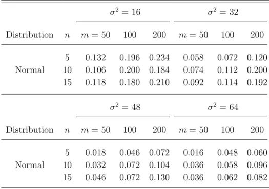
The results shown in Table 1 indicate that the test exhibits a reasonable type I error rate in most sample sizes and cluster sizes with an extremely large variance of the random-effects distribution (σ2 = 64). However, in the scenario of less large or large
variance (σ2 = 16 or 32), it shows a considerable inflation on the type I error rate even
if we try to enhance the amount of information available by increasing the cluster size or sample size.
Table 1. Results of the type I error rate using the asymptotic distribution ofTRS,m for three cluster sizes when σ2=16, 32, 48 and 64.
σ2 = 16 σ2 = 32 Distribution n m= 50 100 200 m= 50 100 200 5 0.132 0.196 0.234 0.058 0.072 0.120 Normal 10 0.106 0.200 0.184 0.074 0.112 0.200 15 0.118 0.180 0.210 0.092 0.114 0.192 σ2 = 48 σ2 = 64 Distribution n m= 50 100 200 m= 50 100 200 5 0.018 0.046 0.072 0.016 0.048 0.060 Normal 10 0.032 0.072 0.104 0.036 0.058 0.096 15 0.046 0.072 0.130 0.036 0.062 0.082
In other words, when the variance component of random effects becomes ex-tremely large and either cluster size or sample size is moderate, the proposed test TRS,m with the ordinary p-value will tend to be less liberal. In this situation, the proposed test is appropriate for testing normality of random effects when the true distribution of random effects is unknown.
3.4.2 Type I Error Rate via Smoothed Bootstrap Test
In order to improve the inflation of the type I error rate shown in Section 3.4.1, the smoothed bootstrap test procedure introduced in Section 3.3.3 is adopted to evaluate the type I error rate of the proposed test TRS,m. Additionally, Racine and MacKinnon (2007), in terms of their simulation experiment, observed that a smoothed bootstrap test will overreject when h is sufficiently small and underreject when h is sufficiently large and the smoothed p-value becomes less sensitive to h when the bootstrap sample size (B) increases. Herein, to avoid overrejection when h is too small and underrejection whenhis too large, we try selected bandwidths not far from h= 1.575B−4/9 which Racine and MacKinnon (2007) used when the test statistic was asymptotically the standard normal, and the cumulative standard Gaussian kernel is adopted. For each simulated data set, the smoothed bootstrap p-value is calculated by
K(w) =
Z w
−∞
k(W)dW,
wherek(W) is the standard normal density and w= ( ˆTRS,m−TˆRS,m∗(l) )/h.
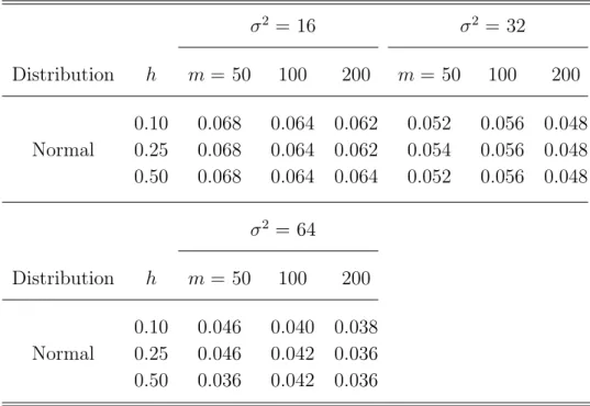
First, we use the bootstrap sample size B = 60 to conduct a small experiment for the cluster sizen= 5 andtij = (−0.1,0,0.1,0.2,0.3). Table 2 reveals that there is no severe overrejection or underrejection and the inflation of type I error rate shown in Table 1 has been improved, even for the less large variance scenario (σ2 =16).
Table 2. Results of the type I error rate using the smoothed bootstrap test procedure with bootstrap sample size B=60 for cluster size n=5 and tij=(−0.1,0,0.1,0.2,0.3) when σ2=16, 32 and 64. σ2 = 16 σ2 = 32 Distribution h m= 50 100 200 m = 50 100 200 0.10 0.068 0.064 0.062 0.052 0.056 0.048 Normal 0.25 0.068 0.064 0.062 0.054 0.056 0.048 0.50 0.068 0.064 0.064 0.052 0.056 0.048 σ2 = 64 Distribution h m= 50 100 200 0.10 0.046 0.040 0.038 Normal 0.25 0.046 0.042 0.036 0.50 0.036 0.042 0.036
Second, we consider another situation with a data set that has cluster sizen= 6 with tij = (0,1,2,4,6,8) (Alonso et al., 2008). Table 3 also indicates that the type I error rate has been well-controlled compared with the prespecified 5% significance level for all sample sizes. Moreover, in Table 4, we observe that performance of the proposed test statistic under the smoothed bootstrap test procedure seems to become much better when the bootstrap sample size increases. Overall speaking, we believe that the proposed test TRS,m with the smoothed bootstrap p-value is reliable for testing normality of the random-effects distribution on this specified model (3.5).
Table 3. Results of the type I error rate using the smoothed bootstrap test procedure with bootstrap sample size B=60 for cluster size n=6 and tij=(0,1,2,4,6,8) when σ2=16 and 32. σ2 = 16 σ2 = 32 Distribution h m= 50 100 200 m = 50 100 200 0.10 0.038 0.038 0.038 0.040 0.062 0.054 Normal 0.25 0.036 0.040 0.038 0.042 0.062 0.054 0.50 0.038 0.040 0.042 0.040 0.062 0.056
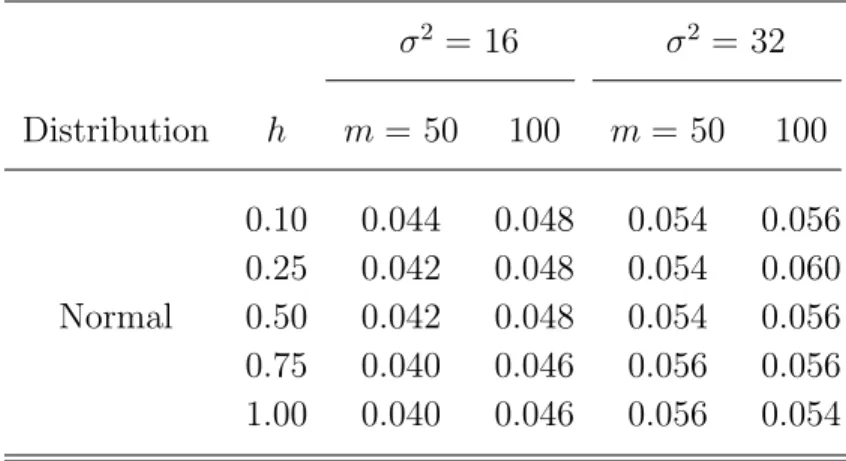
Table 4. Results of the type I error rate using the smoothed bootstrap test procedure with bootstrap sample size B=100 for cluster sizen=6 andtij=(0,1,2,4,6,8) when σ2=16 and 32. σ2 = 16 σ2 = 32 Distribution h m= 50 100 m= 50 100 0.10 0.044 0.048 0.054 0.056 0.25 0.042 0.048 0.054 0.060 Normal 0.50 0.042 0.048 0.054 0.056 0.75 0.040 0.046 0.056 0.056 1.00 0.040 0.046 0.056 0.054
3.4.3 Power Analysis via Smoothed Bootstrap Test
In this part, we evaluate the power performance of the proposed test statisticTRS,m. Herein, six alternative distributions of random effects, including mixture, skewed or heavy-tailed distributions, are generated and adjusted with variance 16 or 32. These distributions are listed as follows:
(1) Mixture normal distribution of 0.3N(−1,12) + 0.7N(6,(21.41/0.7)2), (2) Skewed mixture distribution of 0.25N(14,102) + 0.75χ2(4),
(3) Discrete distribution withp(bi = 1) = 1/6,p(bi = 2) = 1/2 andp(bi = 3) = 1/3, (4) Gamma distribution with shape 1/2 and scale 8,
(5) t distribution with degrees of freedom 4, (6) Lognormal distribution.
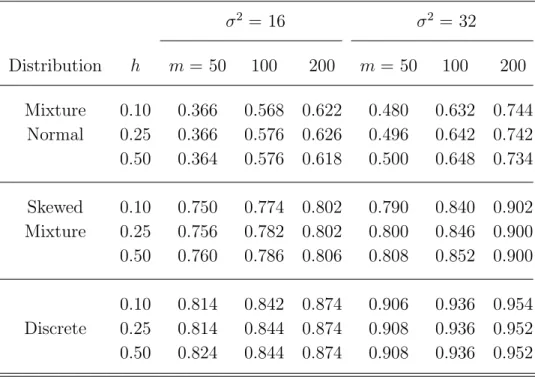
In addition, all simulation results are based on the bootstrap smoothed test procedure with bootstrap sample size B = 60 and generated data with cluster size n = 6 and tij = (0,1,2,4,6,8). Table 5 exhibits a large power for bimodal or multimodal alternatives, especially, when the random-effects distribution possibly follows a skewed mixture distribution or a discrete distribution with 3 support points. Table 5. Results of the power performance of bimodal and multimodal alternatives us-ing the smoothed bootstrap test procedure with bootstrap sample size B=60 for cluster size n=6 andtij=(0,1,2,4,6,8) when σ2=16 and 32.
σ2 = 16 σ2 = 32 Distribution h m= 50 100 200 m = 50 100 200 Mixture 0.10 0.366 0.568 0.622 0.480 0.632 0.744 Normal 0.25 0.366 0.576 0.626 0.496 0.642 0.742 0.50 0.364 0.576 0.618 0.500 0.648 0.734 Skewed 0.10 0.750 0.774 0.802 0.790 0.840 0.902 Mixture 0.25 0.756 0.782 0.802 0.800 0.846 0.900 0.50 0.760 0.786 0.806 0.808 0.852 0.900 0.10 0.814 0.842 0.874 0.906 0.936 0.954 Discrete 0.25 0.814 0.844 0.874 0.908 0.936 0.952 0.50 0.824 0.844 0.874 0.908 0.936 0.952
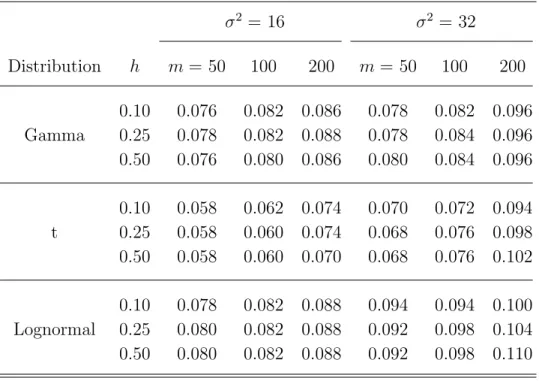
However, in Table 6, it shows that when the random-effects distribution possibly follows a skewed or heavy-tailed unimodal alternative, the proposed test TRS,m has poor power for testing normality of random effects for this specified model (3.5), especially in a scenario of the less large variance (σ2=16) t distribution.
Table 6. Results of the power performance of skewed and heavy-tailed alternatives us-ing the smoothed bootstrap test procedure with bootstrap sample size B=60 for cluster size n=6 andtij=(0,1,2,4,6,8) when σ2=16 and 32.
σ2 = 16 σ2 = 32 Distribution h m= 50 100 200 m = 50 100 200 0.10 0.076 0.082 0.086 0.078 0.082 0.096 Gamma 0.25 0.078 0.082 0.088 0.078 0.084 0.096 0.50 0.076 0.080 0.086 0.080 0.084 0.096 0.10 0.058 0.062 0.074 0.070 0.072 0.094 t 0.25 0.058 0.060 0.074 0.068 0.076 0.098 0.50 0.058 0.060 0.070 0.068 0.076 0.102 0.10 0.078 0.082 0.088 0.094 0.094 0.100 Lognormal 0.25 0.080 0.082 0.088 0.092 0.098 0.104 0.50 0.080 0.082 0.088 0.092 0.098 0.110
Nevertheless, Liti`ere et al.(2008) showed that an asymmetric mixture of two nor-mals random-effects distribution has more severe influence than some non-normal uni-modal random-effects distributions on maximum likelihood estimators of the between-subject effect under assumption of normality of random effects. As a result, it is nec-essary that a proposed test has power for detecting this misspecified random-effects distribution. Fortunately, our proposed test is very powerful for detecting this type of misspecification of the random-effects distribution.
3.5 Application
In this section, we shall apply our proposed test to revisit a data set obtained from a case study in mental health (Alonso et al., 2004). Alonso et al. (2008) had ap-plied their proposed tests on testing normality of the random-effects distribution to this data set. The data collection is briefly sketched as follows. In this case study, the authors studied the effect of risperidone compared to an active control for the treatment of chronic schizophrenia on 128 patients. During the period of the trial, half of patients were assigned to the treatment group; the others were assigned to the control group. Each patient was measured at the following time points: 0, 1, 2, 4, 6 and 8 weeks. For each measurement, the patient’s mental condition was classified as normal to mildly ill (y = 1) or moderately to severely ill (y = 0) where y is a binary response variable. In our analysis, we consider two data structures as follows:
(1) The balanced data is the part of original data set (66 patients) without any missing measured responses at each time point.
(2) The unbalanced data set is the original data set (128 patients) where some patients had missing observed responses at some time points.
Earlier, someone proposed a straightforward diagnostic tool, using empirical Bayes (EB) estimates of random effects to detect departures from normality. We review this basic idea as described by Molenberghs and Verbeke (2005, page 268) as follows. Let us recall the conditional density of response variables shown in Section 2.1. The estimation of random effects is based on their posterior distribution with the following density distribution,
fi(bi|yi,β, D, φ) =
fi(yi|bi,β, φ)f(bi|D)
R
fi(yi|bi,β, φ)f(bi|D)dbi
The estimator of random effects, ˆbi, is the value ofbithat maximizesfi(bi|yi,β, D, φ) where the unknown parameters, β, D and φ, have been replaced by their maximum likelihood estimators based on the likelihood function shown in Section 2.2.
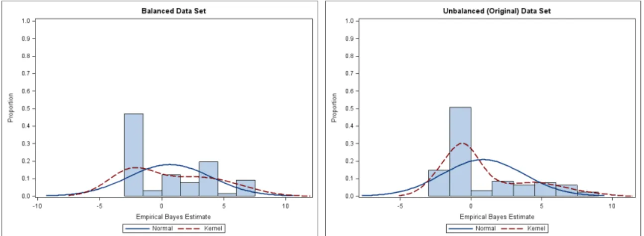
Alonso et al. (2008) provided a histogram plot of the EB estimates of random effects based on the specified model (3.5) for the unbalanced (original) data set shown on the right of Figure 1. Herein, we also provide a histogram plot of the EB estimates for the balanced data set shown on the left of Figure 1. Obviously, it seems to reveal that normality of random effects is questionable on these two data sets. However, it can be shown that in generalized linear mixed model, the empirical Bayes estimates no longer follow a normal distribution, even while the random-effects distribution is correctly specified as normal (Liti`ere et al., 2007; Alonso et al., 2008).
Figure 1. The distribution of empirical Bayes estimates of random effects based on the specified model (3.5) for balanced and unbalanced data sets in mental health study.
Therefore, in order to avoid making an error, we should use a formal proce-dure to test normality of the random-effects distribution. In the following, we ap-ply our proposed test statistic and adopt the smoothed bootstrap test procedure to