Statistical models and inference for dynamic networks

(1)

c

(2)

STATISTICAL MODELS AND INFERENCE FOR DYNAMIC NETWORKS

BY

DANIEL K. SEWELL

DISSERTATION

Submitted in partial fulfillment of the requirements

for the degree of Doctor of Philosophy in Statistics

in the Graduate College of the

University of Illinois at Urbana-Champaign, 2015

Urbana, Illinois

Doctoral Committee:

Associate Professor Yuguo Chen, Chair

Associate Professor Feng Liang

Professor John Marden

Professor Annie Qu

(3)

Abstract

Dyadic data are ubiquitous and arise in the fields of biology, epidemiology, sociology, and many more. Such dyadic data are often best understood within the framework of networks. Network data can vary in many ways. For example, one might have binary or weighted networks, directed or undirected networks, and static or longitudinal networks. This last type of network, also called a dynamic network, is the focus of this work, with the goal of developing important tools and methodology for the analysis of dynamic networks.

A general framework is developed for modeling dynamic networks via a latent space approach. Using a latent space approach to model such networks allows the researcher to model both the local and global structure of the network, inherently accounts for transitivity, and yields rich and meaningful visualization which can easily be interpreted for qualitative inference on the network. A Markov chain Monte Carlo (MCMC) estimation method within a Bayesian setting is presented. Sev-eral useful tools for the researcher arise from this estimation method. First, a method of predicting future relations, or edges, is given. Second, missing data can easily be incorporated into the model, obtaining a posterior probability of each missing edge. Third, a novel concept called nodal influence is introduced which describes how one actor can influence the edges of another actor. Detection of such nodal influence is given via computationally efficient posterior estimation. This model is shown to outperform the existing method, as well as being able to handle richer and more complex data than the existing method. The MCMC algorithm is made scalable by utilizing a log likelihood approximation proposed in the literature, slightly adapted to allow for missing data.

Many of the dynamic networks that arise inherently have weighted edges. The latent space model is extended to handle a variety of types of weighted edges which arise. In particular, the

(4)

algorithms scalable for weighted networks.

Of particular interest is Newcomb’s fraternity data, a network which captures the evolution and formation of a network beginning in its most nascent form and and ending at a stabilized form. The previous model is modified in two non-trivial ways; the first allows for the modeling of rank-order data, which does not fall into the broad categories of weighted network data given previously, and the second allows for the estimation of the evolution of the stability of the network. Next, it is shown how to use the uncertainties associated with the posterior estimation for subgroup detection and for determining the time at which these subgroups formed. Finally, the model parameters are used to find the association between individual stability and popularity.

A longitudinal mixture model is described which can be used to make hard or soft clustering assignments forp-dimensional real valued data. This model accounts for temporal dependence of both the clustering assignment and the object to be clustered. Additionally, the model allows for covariates which may aid in explaining the clustering assignments. The solutions for implementing the generalized EM algorithm are presented. Recursive relationships are derived which allow the computational cost to grow linearly with time rather than exponentially.

The latent space framework and the longitudinal clustering model are combined to perform community detection within dynamic network data, where the communities’ characteristics are fixed but the membership of each community can evolve over time. This method can handle directed or undirected weighted dynamic network data. For community detection within directed or undirected binary networks, a novel model is given along with an efficient variational Bayes estimation algorithm. Both methods are shown to have better performance than using community detection methodology which does not borrow information across time.

(5)

Acknowledgments

I would like to thank my advisor, Dr. Yuguo Chen, for spending countless hours working with me and my numerous manuscript drafts, for acquiring funding support, and most of all for teaching me how to better conduct research and write research articles. I would also like to thank Dr. Annie Qu for supporting and working with me via the consulting office, through which I obtained the initial motivation for Chapter 5 of this manuscript. I would also like to thank Drs. Feng Liang and John Marden for being willing to serve on my graduate committee, giving up their time to thoughtfully consider my research.

I would finally like to express my gratitude towards my wife Marnie for being supremely patient and encouraging, all while enduring Spousal Income Frustration Syndrome, and also towards my parents and my grandmother who financially helped me through my first years of higher education.

(6)

Introduction

Longitudinal relational, or dyadic, data arise in a variety of fields, examples of which include soci-ology, bisoci-ology, computer science, entomology and engineering. This type of data, called dynamic network data, consists of a set of actors and a sequence of sets of relations between the actors called “edges” corresponding to observations at discrete time points. Analyzing dynamic networks is key to seeing how friendships form or dissolve, how politicians form loyalties or break ranks with their parties, how co-authorship patterns develop and change over time, etc.

There exist numerous methods of modeling network data within a statistical framework. Some of these models are intended for static networks but have generative processes which can be thought of as dynamic, in the sense of building up the graph over a series of time points. Examples of this notion can be found in the rewiring of “small-world” networks (Watts and Strogatz, 1998), the subsequent addition of edges in an Erd¨os-R´enyi random graph model (Durrett, 2007), or the addition of nodes and edges in a duplication-attachment model (Kumar et al., 2000). Other methods were developed for static networks and were then extended for the dynamic case. One of the most well known methods of analyzing static networks is the exponential random graph model (ERGM) developed by Frank and Strauss (1986), and much attention is still being given to this class of models (see, e.g., Robins et al., 2007). This was extended to analyzing networks observed over discrete time intervals by Hanneke et al. (2010) in the introduction of the temporal ERGM, or TERGM. Using continuous time Markov processes, Snijders (1996) began a series of works corresponding to what is known as stochastic actor-oriented models. These two approaches focus on the use of common network structures or user-defined objective functions. The last commonly used approach to modeling networks that will be mentioned is the latent space model. Latent space approaches aim to embed network information into some latent space (usually a low dimensional Euclidean space). Benefits of using such an approach is that both local and global structures are modeled, transitivity is inherently incorporated in the model, meaningful visualizations are obtained, and the output is easily interpreted, lending itself to much qualitative inference. While the bulk of the literature on

(9)

latent space models is concerned with static networks, in this dissertation this approach will be used to model longitudinal network data.

The ideas behind latent space models have long been in use. For example, Nakao and Romney (1993) used multidimensional scaling to visualize and analyze the latent positions of the nodes in Newcomb’s fraternity data (Newcomb, 1956). Two formal latent space models were introduced for static networks by Hoff et al. (2002), one of which placed the latent node positions within a Euclidean space, the other placed the latent locations on a unit hypersphere while giving each node an activity level. This latter model was intended to allow for a lack of reciprocity in directed networks. Estimation was performed using Markov chain Monte Carlo (MCMC), hence giving the full posterior of parameters and latent positions. Handcock et al. (2007) expanded the Euclidean model of Hoff et al. (2002) by allowing the latent space positions to follow a mixture of normals, hence allowing clustering to occur simultaneously with embedding in a Euclidean space. Krivitsky et al. (2009) expanded on this work by allowing asymetrical edge probabilities. Schweinberger and Snijders (2003) used a similar approach as Hoff et al. (2002) but used an ultrametric space rather than a Euclidean or hypersphere space to perform model-based clustering. Further work was done in Hoff (2005), where the author extended previous notions of ANOVA models of networks by including as interaction effects the hypersphere latent positions from Hoff et al. (2002).

A limited number of works has considered the temporal aspect of networks while implementing a latent space approach. Robinson and Priebe (2012) presented a method of discovering change points in network behavior via using ak-dimensional simplex latent space. Foulds et al. (2011) developed a non-parametric infinite feature model, where the features are latent. The work most related to the model that will be proposed in Chapter 2 is that of Sarkar and Moore (2005), which extended the Euclidean latent space model of Hoff et al. (2002) to (undirected) dynamic networks. They developed a generalized multidimensional scaling (GMDS) to find the initial latent node positions across discrete time points. The authors then furthered this by using a conjugate-gradient method of optimizing an objective function,. While this is a speedy algorithm and hence can be used for larger data sets, the estimation is based on a filtering-like algorithm (hence not all the data is used for estimating the latent positions) which in the end leads to estimates that are not statistically meaningful. The models in Chapters 2 and 3 extend this to broader contexts while better modeling

(10)

structure, both local and global, and the evolution of the network. The estimation is done in a Bayesian framework which allows for prediction, missing data, and detection of nodal influence. Chapter 3 shows how to extend this model for weighted dynamic network data. Specifically, the model is extended for the case where the edges belong to an exponential family of distributions; also is shown the case where a similar strategy can be employed through data augmentation. Chapter 4 takes a close look at Newcomb’s fraternity data. This is a longitudinal network data set which uniquely captures the evolution of a network as it transitions from an unformed state (all actors were unacquainted) to a stabilized form. With this data I employ novel strategies for determining the time at which the network stabilizes, the time at which subgroups form, and the association between individual stability and popularity. Chapter 5 provides a method of clustering longitudinal

p-dimensional real valued data, providing numerically efficient ways of computing the likelihood and an estimation method employing the generalized EM algorithm. Chapter 6 provides two methods of community detection in dynamic networks. The first method combines the models of Chapters 2, 3 and 5 for a model that allows the detection of communities in directed or undirected weighted or binary dynamic networks. The second method is a novel model and estimation algorithm for community detection within binary directed or undirected dynamic networks. In both cases, as in Chapter 5, the structure of each community is assumed fixed but the community memberships are allowed to vary with time.

(11)

Chapter 2

Latent Space Model for Binary

Dynamic Networks

Network analysis, and in particular dynamic network analysis, is a ubiquitous area of study, used by scientists in many distinct fields (Vivar and Banks, 2011). Often studied are dynamic social networks, which come in a wide variety of forms (see the Special Issues on Network Dynamics in Social Networks, January 2010 and July 2012). Dynamic networks are also analyzed in epidemiological contexts (Bansal et al., 2010), in analyzing terrorist networks (Carley, 2006), and much more.

In this chapter, we propose a model which embeds dynamic directed, or undirected, network data into a latent Euclidean space, allowing each node to have a temporal trajectory in this latent space. Estimation of the model parameters and latent nodal positions occur within a Bayesian framework using MCMC. By using our approach, the user can observe much more easily how the network evolves over time, gain insight into global and local structures, handle missing data, make future predictions, and can detect the attracting influence one actor has on another actor’s friendships (a concept we call nodal influence, which will be discussed later). To improve the speed of the MCMC algorithm for large networks, we describe an approximation method which reduces the computational cost.

The remainder of the chapter is organized as follows: Section 2.1 describes the proposed model for dynamic networks. Section 2.2 outlines the Bayesian estimation of the model parameters and latent nodal positions, as well as addressing the issue of scalability. Section 2.3 details how to handle missing data. Section 2.4 describes how to obtain network predictions. Section 2.5 gives a method for detecting and visualizing nodal influence. Section 2.6 shows simulation results. Section 2.7 presents the results from analyzing data collected from a Dutch classroom as well as from analyzing cosponsorship data collected on members of the U.S. House of Representatives. Sections 2.8 and 2.9 gives the proofs of the lemmas given earlier in the chapter.

(12)

2.1 Dynamic Latent Space Model

We assume that data come in the form of (_N,_{Et:t∈ T }), whereN is the set of all nodes, andEtis the set of edges at timet. For simplicity let_T =_{1,2, . . . , T_}. For the majority of the chapter it will also be assumed that_Etconsists of directed edges. The general idea of the latent space approach is that this time series of graphs can be represented as a state space model, with a latent state variable representing the nodes as positions in a low dimensional Euclidean space. The closer two nodes are in this latent Euclidean space, the more likely they are to form an edge. This low dimensional space can be thought of as a characteristic space where the distance between nodes represents how similar they are (Hoff et al., 2002), or as a social space where the distance between two nodes corresponds to the strength of the relationship between the two.

The notation to be used throughout the rest of the chapter is as follows: n=_{|N |}is the number of nodes. For a latent space_<p_,_X

it is thepdimensional vector of theithnode’s latent position at timet, and _Xtis then×pmatrix whoseithrow isXit. Yt={yijt} is the adjacency matrix of the observed network at timet, andyijt = 1 if there is an edge from nodeito node j at timet and 0 otherwise.

The latent node positions are modeled by a Markov process with the initial distribution

π(_X1|ψ) = n

Y

i=1

N(Xi1|0, τ2Ip), (2.1)

and transition equation

π(_Xt|Xt−1,ψ) = n

Y

i=1

N(Xit|Xi(t−1), σ2Ip) (2.2) fort= 2,3, . . . , T, whereIp is thep×pidentity matrix, N(x|µ,Σ) denotes the normal probability density function with meanµand covariance matrix Σ evaluated atx, andψis a vector of parameters which will be defined shortly.

The observed networks at different time points are conditionally independent given the latent positions. This dependence structure is illustrated in Figure 2.1. Further, it is assumed that for any two (distinct) pairs (i, j) and (i0, j0), yijt and yi0_j0_t are independent conditioning on (X_t,ψ).

In formulating the observation equation of our model, we desire two main properties: first, the probability of an edge from actorito actorjat timetshould increase as the distance between their latent positions decreases; second, the probability of an edge should depend on both who is sending and who is receiving the link, and we should further be able to determine the importance of each

(13)

in edge formation; i.e., whether the identity of the sender or the identity of the receiver is more important in edge formation. To this end, we use the formulation

P(Yt|Xt,ψ) =

Y

i6=j

P(yijt = 1|Xt,ψ)yijt·P(yijt= 0|Xt,ψ)1−yijt =

Y

i6=j

exp(yijtηijt)

1 + exp(ηijt), (2.3) where ηijt,log P(yijt = 1|Xt,ψ) P(yijt = 0|Xt,ψ) =βIN 1₋dijt rj +βOU T 1₋dijt ri , (2.4)

and dijt =kXit−Xjtk and ψ = (τ2, σ2, βIN, βOU T, r1:n) are the model parameters. Herer1:n = (r1, r2, . . . , rn); similar notation will be used throughout the rest of the chapter. βIN andβOU T are global parameters which reflect the importance of popularity and social activity respectively. The

ri’s are positive node specific parameters that represent each node’s social reach and is reflective of the tendency to form and receive edges. Within the latent space, there is also the geometrical interpretation of ri forming a radius around the ith node, as we will see later. For model identi-fiability, the ri’s are constrained so that Pn

i=1ri = 1. This parameterization emulates both the distance and projection models of Hoff et al. (2002) for static networks, given asηij =β(1−dij) andηij =β+Xi0Xj/kXjk respectively, by utilizing the visually appealing and intuitive Euclidean space for the latent positions while incorporating the individual actors’ “sociability,” or social reach, while also accounting for both activity and popularity.

Krivitsky et al. (2009) built onto Hoff et al.’s model by including additive random individual effects. Here our parameterization links the actors’ individual effects to the latent space, in the sense that the social reach dampens or augments the effect of the distance between the two actors, rather than having the individual actor effects be constant additive effects; thus these two parameterizations are in fact different, rather than being subsets of each other. In some sense their model is more flexible in that an actor has both an indegree effect and an outdegree effect. Our model can be trivially extended to account for this by simply allowingr1:n to be replaced by two sets of parametersr

(IN) 1:n andr_1:n(OU T). We applied this more complex model on the two real data sets presented in Section 2.7 with no improvement in model fit. Hence our focus remains on the simpler model, given in (2.4).

(14)

(_X1,Ψ) (X2,Ψ) (X3,Ψ) . . .

Y1 Y2 Y3

Figure 2.1: Illustration of the dependence structure for the latent space model. Yt is the observed graph,_Xtis the unobserved latent node positions, andψ is the vector of model parameters.

radius within the latent social space of the ith node’s social reach. This is evident in that if the distance between two nodes are within each other’s radii, i.e.,dijt<min(ri, rj), then the probability of an edge is greater than 1/2; if they are outside each other’s radii, i.e., dijt > max(ri, rj), then the probability of an edge is less than 1/2; and if the distance between the two nodes equals both radii, i.e.,dijt=ri=rj, then the probability of an edge equals 1/2. These scenarios are illustrated in Figure 2.2. Thus in case (1), a larger radius implies an increasing propensity to send and receive ties. This fact is illustrated in Figure 2.3a, where the probabilityP(yijt = 1|Xt,ψ) is shown in a contour plot, allowingri andrj to vary, with distancedijt= 0.01,βIN = 2 andβOU T = 1/2. Now ifβIN > βOU T (βOU T > βIN) then we can conclude that the probability of an edge from nodei to nodej (from nodej to node i) is determined more by the radius ofj than by the radius ofi. This is also illustrated in Figure 2.3a, where it is apparent that the probability of an edge from i to j

increases much faster when we fix a value of ri and allowrj to increase than vice versa. Thus in case (1), if βIN > βOU T then the edges of the network are determined more by the popularity of the actors than by their activity, i.e., the identity of the receiver of the edge is more important than the identity of the sender, and ifβOU T > βIN the edges of the network are determined more by the activity of the actors than by their popularity, i.e., the identity of the sender is more important than the identity of the receiver.

In case (2), one of the β coefficients is negative; without loss of generality assume βOU T <0 andβIN >|βOU T|. Considering the probability of an edge from nodei to nodej, note that as rj increases the probability of an edge increases; thus in case (2), a larger radius implies an increasing propensity to receive ties. This is illustrated in Figure 2.3b, where P(yijt = 1|Xt,ψ) is shown in a contour plot, allowingri and rj to vary, with distancedijt = 0.01, βIN = 2 and βOU T =−1/2. Similar to case (1), the probability of an edge from nodeito nodej is determined more byrj than

ri. This can be seen in Figure 2.3b where it is apparent that when we fixri and allowrjto increase,

(15)

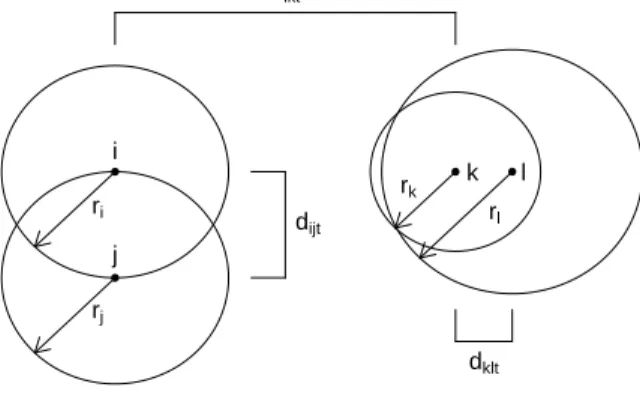
● ● ● ● i j k l ri rj rk rl dijt dklt dikt

Figure 2.2: Illustration of how to interpret social reach parametersr1:nin the case thatβIN, βOU T > 0; the probability of an edge fromitok is less than 1/2, fromkto lis greater than 1/2, and from

itoj is equal to 1/2.

when we fixrj and allowri to increase. Thus in case (2) the edges of the network are determined more by the popularity of the actors than by their activity. Similar conclusions can be made if we assumeβIN<0 andβOU T >|βIN|.

Any other case than these two would contradict the intuition of the model that a shorter distance between two nodes is guaranteed to lead to an increased probability of an edge; additionally the possibility of groups of nodes (communities) would no longer exist.

r

j 0.005 0.010 0.015 ●

r

j 0.005 0.010 0.015 ●

(16)

2.2 Estimation

We adopt a Bayesian approach, and hence we wish to make inferences based on π(_X1:T,ψ|Y1:T), where ψ = (τ2_{, σ}2_{, β}

IN, βOU T, r1:n). We implement a Metropolis-Hastings (MH) within Gibbs MCMC scheme as suggested by Geweke and Tanizaki (2001) to sample from the posterior, hence giving point estimates and uncertainties. We set the priors on the parameters as follows: as-sume that βIN ∼ N(νIN, ξIN), βOU T ∼ N(νOU T, ξOU T), σ2 ∼ IG(θσ, φσ), τ2 ∼ IG(θτ, φτ) and (r1, r2, . . . , rn)∼Dirichlet(α1, α2, . . . , αn), whereIGis the inverse gamma distribution. The inverse gamma priors were chosen to be conjugate, and the Dirichlet prior is a natural selection for such constrained parameters.

2.2.1 Initialization

The number of MCMC iterations required to reach convergence can be greatly reduced by appro-priate initial values of the latent positions_X1:T and the parameters τ2,σ2, βIN, βOU T, andr1:n.

We want the radiir1:n, or social reaches, to be strongly associated with the in and outdegree of the nodes. Therefore we have the initial estimates (denoted by superscript(1)) of each radius to be

r_i(1)=

PT

t=1

P

j6=i(yijt+yjit)/2

PT

t0₌₁

P

j0_6=i0yi0_j0_t0

. (2.5)

A nice method of obtaining initial latent positions _X_1:T(1) is GMDS, given by Sarkar and Moore (2005). This GMDS method extends the classical multidimensional scaling (CMDS) by using CMDS to obtain_X₁(1), and then fort= 2,3, . . . , Tminimizing an objective function that balances the CMDS estimates for _X_t(1) with the previous estimates of _X_t−1(1). To perform GMDS, T distance matrices {dijt}are required; Sarkar and Moore suggested constructing these distance matrices by settingdijt to be the length of the shortest path fromitojat timet. We too do this, though we rescale by 1/n

to keep the distances on the same scale as the radii, as (2.4) seems to suggest is necessary. From the initial estimates of the radii and the latent positions, we find initial estimates ofβIN andβOU T by maximizing the likelihood numerically.

An intuitive initial value forτ2_{can be found using the initial latent positions}

X1(1)in the following way: 1 np n X i=1 kX(1)_i1 _k2. (2.6)

One could determine the initial value forσ2 _{by using the initial positions}

(17)

way as was done for τ2. Note that such an initial estimate would be heavily influenced by the user specified tuning parameter in the GMDS algorithm, and hence the user may be misled into thinking that the data are supporting a particular initial value when in fact the user has already predetermined it. In our simulation study and real data analyses we chose a large initial value for

σ2 _{in order to allow the latent positions} _X

it to move more during the beginning iterations of the MCMC algorithm.

There typically is no intuition as to what values to set the hyperparameters of the prior distri-butions, and so we suggest using some of these initial values of the parameters to aid in this. To make the prior ofτ2flat one can set the shape and scale parameters of the inverse gamma prior to be respectivelyθτ= 2 +δandφτ= (1 +δ)·E(τ2) for some smallδ >0, whereE(τ2) is set to be the

initial estimate in (2.6). The initial estimates ofβIN andβOU T are natural selections for νIN and

νOU T. The prior can then be made flat by simply choosing ξIN and ξOU T to be very large values. The hyperparameters forr1:n may all be set equal to 1 in order to obtain a flat and uninformative prior, as well as to simplify the computations involved in the MCMC algorithm. There are no auto-matic decisions for determining the hyperparameters forσ2_{. However, as we will see in Section 2.6,} the MCMC algorithm is not sensitive to this selection.

2.2.2 Posterior Sampling

To sample via Metropolis-Hastings within Gibbs algorithm, we draw from the full conditional dis-tributions iteratively. These conditional disdis-tributions are either known in closed form or up to a normalizing constant and are given below.

Lettingpijt,P(yijt|Xt,ψ) = exp(yijtηijt)/(1 + exp(ηijt)), the conditional distribution forXitis

π(Xit|Y1:T,ψ)∝               

(

Q j:j6=i

pijtpjit

)

·N(Xit|0, τ2Ip)·N(Xi(t+1)|Xit, σ2Ip), ift= 1

(

Q

j:j6=i

pijtpjit

)

·N(Xi(t+1)|Xit, σ2Ip)·N(Xit|Xi(t−1), σ2Ip), if 1< t < T

(

Q

j:j6=i

pijtpjit

)

·N(Xit|Xi(t−1), σ2Ip), ift=T . (2.7)

(18)

The conditional distributions forβIN andβOU T are π(βIN|Y1:T,X1:T, τ2, σ2, βOU T, r1:n) ∝   T Y t=1 Y i6=j pijt  ·N(βIN|νIN, ξIN), (2.8) π(βOU T|Y1:T,X1:T, τ2, σ2, βIN, r1:n) ∝   T Y t=1 Y i6=j pijt  ·N(βOU T|νOU T, ξOU T). (2.9)

Assuming the prior ofr1:n is Dirichlet(1, . . . ,1), the conditional distribution forr1:n is

π(r1:n|Y1:T,X1:T, τ2, σ2, βIN, βOU T)∝ T Y t=1 Y i6=j pijt. (2.10)

The conditional distributions forτ2 andσ2 are

τ2|Y1:T,X1:T, σ2, βIN, βOU T, r1:n ∼ IG θτ+np/2, φτ+ 1 2 n X i=1 kXi1k2 , (2.11) σ2|Y1:T,X1:T, τ2, βIN, βOU T, r1:n ∼ IG θσ+np(T−1)/2, φσ+1 2 T X t=2 n X i=1 kXit−Xi(t−1)k2 . (2.12)

The posterior sampling algorithm is then

0. Set the initial values of (_X1:T,ψ) (e.g., to those described in Section 3.1).

1. Fort= 1, . . . , T and fori= 1, . . . , n, drawXitvia MH using a normal random walk proposal.

2. Drawτ2 from (2.11).

3. Drawσ2_{from (2.12).}

4. DrawβIN via MH using a normal random walk proposal.

5. DrawβOU T via MH using a normal random walk proposal.

6. Drawr1:n via MH using a Dirichlet proposal. Repeat steps 1-6.

Due to the constraint on the radii (Pn

i=1ri= 1), it is necessary to, within the MH step, accept or reject alln values simultaneously; hence it is important to keep the movements small, i.e., the variance of the proposal small. We also desire to keep the means at the current values. Therefore the proposal used to draw the new values r∗1:n is another Dirichlet distribution with parameters (κr1, κr2, . . . , κrn), where the ri’s are the current values and κ is some large constant. Thus the acceptance rate forr∗_1:n is

min 1,π(r ∗ 1:n|Y1:T,X1:T, τ2, σ2, βIN, βOU T) π(r1:n|Y1:T,X1:T, τ2, σ2, βIN, βOU T)· Dir(r1:n|κr1:n∗ ) Dir(r_1:n|∗ _κr 1:n) ,

whereDir(r1:n|α1:n) is the Dirichlet probability density function with parametersα1:n evaluated at

(19)

One last note is that the posterior will be invariant to rotations, reflections, and translations of the latent positions. Hence any inference must take into account the non-uniqueness of the estimates. Similar to the approach described in Hoff et al. (2002), we perform a Procrustes transformation to reorient the sampled trajectories. We set an (nT)_×p reference trajectory matrix X0, and after drawing new Xit for all i and t, we construct from these new draws the new trajectory matrix

X = (_X₁0, . . . ,_X_T0)0. In practice we used the initial latent positions to constructX0. The Procrustes transformation onX usingX0 as the target matrix finds

argmin

X∗

tr(X0−X∗)0(X0−X∗),

whereX∗is some rotation and translation ofX; see, e.g., Borg (2005). By performing the Procrustes transformation on the trajectory matrix, we obtain a single rotation matrix A with which we use to setX(`)=XA, where the superscript(`)_{denotes the stored values for the}_`th_{iteration; that is,} we setX(`)_it =A0Xit. By so doing we are preserving the distances between any actors at any time points, i.e.,_kX(`)_it ₋X(`)_js_k=_kXit−Xjskfor any actorsiandj and any time points tands.

2.2.3 Scalability

Scalability is an issue for latent space models for network data. For static networks, this issue has been addressed through using variational Bayes (Salter-Townshend and Murphy, 2012) and also by using case-control principles from epidemiology (Raftery et al., 2012). This latter method reduced the computational cost (for static networks) of computing the log likelihood fromO(n2_{) to}_O₍_n_).

The general strategy of the case-control log likelihood approximation is to write the log likelihood as two summations. Assuming that the network becomes sparser asngets larger, the computational cost of the first of the two summations is linear with respect to n, and the cost of the second is quadratic. The second summation is then replaced by a Monte Carlo estimate obtained from a subsequence of the actors, thus making the overall cost of computing the log likelihood linear inn. This method as described by Raftery et al. (2012), however, cannot be directly extended to longitudinal network data containing missing edge values which is often the case, especially in social networks. This is because all the links need to be known a priori. By modifying how the log

(20)

One can reduce the computational cost involved in an iteration of the MCMC algorithm by approximating the acceptance ratios corresponding to the Metropolis-Hastings steps. Consider the latent positions where, for actoriat timet, it is necessary to computeQ

j:j6=ipijtpjit. We can write the log of this quantity as three summations:

X

j:j6=i

log(pijtpjit) =

X

j:j6=i

yijtηijt+yjitηjit−log(1 + exp(ηijt))−log(1 + exp(ηjit))

= X j:yijt=1 ηijt+ X j:yjit=1 ηjit− X j:j6=i

log(1 + exp(ηijt)) + log(1 + exp(ηjit))

.

(2.13) From this expression we see that for each MCMC iteration it is necessary to compute O(T n2₎ terms for updating _X1:T. It is reasonable, though, to assume that as n gets larger the adjacency matrices become sparser, and so the first two summations are not growing at an alarming rate; we can formalize this by assuming that either the maximum node degree is fixed or is of o(n). The final summation in (2.13), however, requires n₋1 calculations, and hence is responsible for the computational cost being quadratic with respect to n. To ease the computational burden, we replace this term with a summation of only a fixed numbern0 of terms. Specifically, we randomly draw for eachia subsequence_{jk}nk=10 . Then the last term in (2.13) can be approximated as

X

j:j6=i

[log(1 + exp(ηijt)) + log(1 + exp(ηjit))]

≈n_n−1 0

n0

X

k=1

[log(1 + exp(ηijkt)) + log(1 + exp(ηjkit))]. (2.14)

A similar approximation can be used in the acceptance ratios forβIN,βOU T andr1:n. For each of these it is necessary to computeQT

t=1

Qn

i=1

Q

j:j6=ipijt. For eachiandt, log

Q

j:j6=ipijt

can be written as two summations:

X

j:j6=i

log(pijt) =

X

j:j6=i

[yijtηijt−log(1 + exp(ηijt))]

= X

j:yijt=1

ηijt−

X

j:j6=i

log(1 + exp(ηijt)). (2.15)

Here again we see that the number of terms to be summed in updating βIN, βOU T and r1:n is of

(21)

approxi-mated as

X

j:j6=i

log(1 + exp(ηijt))≈

n₋1 n0 n0 X k=1 log(1 + exp(ηijkt)). (2.16)

By using the approximations in (2.14) and (2.16), the computational cost of each MCMC iteration is reduced fromO(T n2) toO(T n), i.e., the computational cost is now linear with respect ton.

It is not necessary to know the values of the yijt’s a priori in order to draw the subsequences {jk}nk=10 . Further, (2.13) can still be calculated because at each iteration of the MCMC algorithm there will be some estimate ofyijt. Therefore this approximation can be implemented in the context of missing data.

One last note is that the sampling of the subsequences_{jk}n_k=10 can be drawn in a variety of ways. In the simulations of Section 2.6 and the cosponsorship data analysis of Section 2.7, the subsequences were drawn via stratified sampling. That is, for eachi, then₋1 other nodes were divided into two groups,G1=

j₆=i:yijt= 1 oryjit= 1 for at least onet andG2=

j₆=i:yijt=yjit= 0, ∀t . Then_{jk}ck=1 was a random sample fromG1and{jk}nk=c+10 was a random sample fromG2, where

c=

n0|G1|/(n−1) + 0.5

.

2.3 Missing Data

Missing data in social networks is not uncommon, and can come in various forms, such as boundary specification, non-response, and censoring by vertex degree (Kossinets, 2006). Here we specifically focus on non-responses, i.e., missing edge values. For static networks there have been a number of methods proposed (see, e.g., Robins et al., 2004; Huisman, 2009). For dynamic networks, Huisman and Steglich (2008) compared several methods to handle missing edges in the context of a stochastic actor oriented model. Handcock and Gile (2010) developed a theoretical framework for networks in which only a subset of the dyads are observed; we use this framework in our discussion and refer the reader to Handcock and Gile’s paper for more details.

Let_Ddenote the sampling pattern; that is, _Dis the set ofn_×nmatrices_{D1, . . . , DT} where

Dijtequals 1 if the dyadyijtis observed and equals 0 otherwise. LettingY(obs)andY(mis)denote the collection of observed edges and missing edges respectively, the complete data is (_Y(obs)_,

Y(mis)_, D),

(22)

unobserved edges depends on the unobserved edges themselves (called non-ignorable missing data) is a difficult scenario which is beyond the scope of this chapter; thus we will continue the discussion assuming that the missing edges are either MCAR or MAR.

Rubin (1976) discussed weak conditions for which it is possible to ignore the process that causes missing data. In our context, we are interested in the posterior distributionπ(_X1:T,ψ,Y(mis)|Y(obs),D); hence if the sampling pattern is ignorable, we may make inference based on the posterior distribu-tionπ(_X1:T,ψ,Y(mis)|Y(obs)), i.e.,X1:T,ψ andY(mis)are independent ofDgivenY(obs). There are two sufficient conditions that must be satisfied in order for the sampling pattern to be ignorable (Rubin, 1976). First, the sampling pattern parameters ξ are a priori independent with the data (_Y(mis),_Y(obs)), latent positions _X1:T and model parameters ψ, i.e., π(Y(mis),Y(obs),X1:T,ψ, ξ) =

π(_Y(mis),_Y(obs),_X1:T,ψ)π(ξ). Second, the space of (ξ,X1:T,ψ) is a product space, i.e., if ξ ∈ Ξ, X1:T ∈ X and ψ ∈ Ψ then (ξ,X1:T,ψ) ∈ Ξ×X ×Ψ. If these two conditions are met and the missing edges are either MCAR or MAR, we have

π(_Y(mis),_X1:T,ψ|Y(obs),D) =

R

π(_D|Y(obs), ξ)π(_Y(mis),_Y(obs),_X1:T,ψ)π(ξ)dξ

R

π(_D|Y(obs)_{, ξ}₎_π₍_Y(obs)₎_π₍_ξ₎_dξ =π(Y (mis)_, Y(obs)_, X1:T,ψ) π(_Y(obs)₎ =π(_Y(mis),_X1:T,ψ|Y(obs)). (2.17)

Handling the missing data is easy when using the MH within Gibbs sampling scheme of Section 3. Using the observed data and the current values for the missing data, the full conditionals for_X1:T andψ are unchanged. The full conditional of_Y(mis) _{is determined by, for any}_y

ijt∈ Y(mis),

π(yijt|X1:T,ψ) =

exp(yijtηijt) 1 + exp(ηijt)

, (2.18)

whereηijt is given in (2.4). That is, including the missing data in the MH within Gibbs sampling amounts to an additional draw for each missingyijt from a Bernoulli distribution with probability determined by (2.4).

2.4 Prediction

Predicting future links is an important and interesting problem. Applications include recommender systems, terrorist networks, protein interaction networks, prediction of friendship networks, and

(23)

more (Wang et al., 2007; Kashima and Abe, 2006; Hopcroft et al., 2011; Liben-Nowell and Kleinberg, 2007).

When considering prediction in the latent space context, it is of interest to predict for timeT+ 1 both the edges of the adjacency matrixYT+1 and the latent space positionsXT+1. It is simple to find point estimates of the latter since

π(_XT+1|Y1:T) = Z π(_XT+1|XT,ψ)π(X1:T,ψ|Y1:T)dX1:Tdψ ≈ _L1 L X `=1 n Y i=1 N(Xi(T+1)|X (`) iT, σ 2(`)_I_p)_, _(2.19)

where the superscript(`) _{indicates the}_`th_{draw from the posterior. Hence}

b XT+1,E(XT+1|Y1:T)≈ 1 L L X `=1 XT(`). (2.20)

It is assumed that an appropriate burn-in period for the chain has been accounted for.

A simple way to compute a point estimate of the probability of an edge betweeniandj at time

T+ 1,_P(yij(T+1)= 1), would be to plug inXbT+1along with the posterior means of the parameters into the observation equation (2.4). We can, however, do a little better by not conditioning on the posterior means of the model parameters, hence eliminating some unnecessary uncertainty. We aim, then, to find _P(YT+1|Y1:T,XT+1 = XbT+1). Since conditional on XT+1 we still assume that the yij(T+1)’s are independent, we need only findP(yij(T+1)|Y1:T,Xbi(T+1),Xbj(T+1)). This can be estimated as follows:

First, we approximate the joint distribution.

P(yij(T+1),Xi(T+1),Xj(T+1)|Y1:T) =

Z

π(yij(T+1)|Xi(T+1),Xj(T+1),ψ)π(Xi(T+1),Xj(T+1)|X1:T,ψ)π(X1:T,ψ|Y1:T)dX1:Tdψ ≈_L1

L

X

`=1

π(yij(T+1)|Xi(T+1),Xj(T+1),ψ(`))π(Xi(T+1),Xj(T+1)|X (`) T ,ψ

(`)₎_. _(2.21)

(24)

andπ(yij(T+1)|Xbi(T+1),Xbj(T+1),ψ) is defined in (2.3) and (2.4).

This method outperforms the simpler plug in method mentioned earlier, as will be seen in Section 2.6 when the simulation results are given. The intuition as to why this is so is that we are using fewer estimated parameters to make predictions, hence introducing less uncertainty into the prediction estimates.

2.5 Nodal Influence

The latent space approach gives rise to a novel way of detecting and viewing nodal, or social, influence. Anagnostopoulos et al. (2008) defined social influence as “the phenomenon that the actions of a user can induce his/her friends to behave in a similar way.” Many authors attempt to use social influence to track the propagation of ideas or behaviors through a network (e.g., Kempe et al. (2003), Leskovec et al. (2006)). Tang et al. (2009) described a method of determining which nodes will influence which other nodes on a variety of topics. Goyal et al. (2010) proposed a method of labeling each edge by an influence probability, assuming undirected binary edges. These works all require data outside of the network, such as, as phrased by Goyal et al., an “action log.” Here we consider nodal influence as the attracting influence one node has on another node’s friendships; i.e., how one person draws another person into their own social circle. Hence our new definition of nodal influence is how one node affects the edges of another node.

We assume that the way in which one node can affect another node’s movements in the network is manifested in an increased tendency for the influenced node to move in the direction of the influencing node in the social space. To detect the tendency for a nodeito move through the social space in the direction of another node j, the transition equation for the latent nodal positions is extended by considering a new parameter to describe the nodal influence between two nodes. We will then carefully define this parameter, implement an appropriate prior, and then look at posterior

(25)

probabilities that will help the user determine whether or not there is nodal influence. We will show that this can be done by using the same MCMC output as when the transition equation was assumed to be a random walk. Throughout the next two sections we consider looking at the nodes pairwise, i.e., we look at whether or not a specific nodeiis influenced by another nodej.

2.5.1 Nodal Influence Detection

Consider an extension of the transition equation (2.2) such that Xit = Xi(t−1)+it where it ∼

N(µt, σ2Ip). In the following, assume thatp= 2. Letθtequal the angle atan2(Xjt−Xi(t−1)), where atan2 is the common variation of the arctangent function which preserves the angle’s quadrant, taking a vector rather than a ratio as its argument. Let_Rt be the rotation matrix associated with

θt. We then letµtbe of the form

µt=Rt    µ 0   =    cos(θt) ₋sin(θt) sin(θt) cos(θt)       µ 0   , (2.25)

where µ= _kE(Xit−Xi(t−1))k is some unknown parameter taking non-negative values. No nodal influence is equivalent to the case whereµ = 0, and if there does exist some nodal influence then this will be reflected in someµ >0. Figure 2.4 gives an illustration of this type of nodal influence. The idea here is that node i will aim towards wherever nodej is within the latent characteristic space. If we let the prior on the parameters (ψ, µ) be independent, i.e., π(ψ, µ) =π(ψ)π(µ), then the posterior samples obtained from Section 2.2.2 can be equivalently viewed as having come from

π(_X1:T,ψ|Y1:T, µ = 0). This is important because, as will be seen later, we can use these same draws to make inference regarding the nodal influence existing between nodesi and j. Also note that under the extended transition equation, the Markov property still holds for the latent positions, i.e.,π(_Xt|X1:(t−1),ψ, µ) =π(Xt|Xt−1,ψ, µ).

The prior distribution of µ is chosen to be a mixture of a point mass on 0 and a continuous component over the positive reals:

π(µ) =     p0 ifµ= 0 (1₋p )f(µ) forµ >0, (2.26)

(26)

● ● ● ● Xi(t−1) Xi(t−1)+ µt Xit Xjt ● ● ● ● ● ● ● ● ● ● ● ● ● ● ● ● ● ● ● ● ● ● ● ● ● ● ● ● ● ● ● ● ● ● ● ● ● ● ● ● ● ● ● ● ● ● ● ● ● ● ● ● ● ● ● ● ● ● ● ● ● ● ● ● ● ● ● ● ● ● ● ● ● ● ● ● ● ● ● ● ● ● ● ● ● ● ● ● ● ● ● ● ● ● ● ● ● ● ● ● ● ● ● ● ● ● ● ● ● ● ● ● ● ● ● ● ● ● ● ● ● ● ● ● ● ● ● ● ● ● ● ● ● ● ● ● ● ● ● ● ● ● ● ● ● ● ● ● ● ● ● ● ● ● ● ● ● ● ● ● ● ● ● ● ● ● ● ● ● ● ● ● ● ● ● ● ● ● ● ● ● ● ● ● ● ● ● ● ● ● ● ● ● ● ● ● ● ● ● ● ● ● ● ● ● ● ● ● ● ● ● ● ● ● ● ● ● ● ● ● ● ● ● ● ● ● ● ● ● ● ● ● ● ● ● ● ● ● ● ● ● ● ● ● ● ● ● ● ● ● ● ● ● ● ● ● ● ● ● ● ● ● ● ● ● ● ● ● ● ● ● ● ● ● ● ● ● ● ● ● ● ● ● ● ● ● ● ● ● ● ● ● ● ● ● ● ● ● ● ● ● ● ● ● ● ● ● ● ● ● ● ● ● ● ● ● ● ● ● ● ● ● ● ● ● ● ● ● ● ● ● ● ● ● ● ● ● ● ● ● ● ● ● ● ● ● ● ● ● ● ● ● ● ● ● ● ● ● ● ● ● ● ● ● ● ● ● ● ● ● ● ● ● ● ● ● ● ● ● ● ● ● ● ● ● ● ● ● ● ● ● ● ● ● ● ● ● ● ● ● ● ● ● ● ● ● ● ● ● ● ● ● ● ● ● ● ● ● ● ● ● ● ● ● ● ● ● ● ● ● ● ● ● ● ● ● ● ● ● ● ● ● ● ● ● ● ● ● ● ● ● ● ● ● ● ● ● ● ● ● ● ● ● ● ● ● ● ● ● ● ● ● ● ● ● ● ● ● ● ● ● ● ● ● ● ● ● ● ● ● ● ● ● ● ● ● ● ● ● ● ● ● ● ● ● ● ● ● ● ● ● ● ● ● ● ● ● ● ● ● ● ● ● ● ● ● ● ● ● ● ● ● ● ● ● ● ● ● ● ● ● ● ● ● ● ● ● ● ● ● ● ● ● ● ● ● ● ● ● ● ● ● ● ● ● ● ● ● ● ● ● ● ● ● ● ● ● ● ● ● ● ● ● ● ● ● ● ● ● ● ● ● ● ● ● ● ● ● ● ● ● ● ● ● ● ● ● ● ● ● ● ● ● ● ● ● ● ● ● ● ● ● ● ● ● ● ● ● ● ● ● ● ● ● ● ● ● ● ● ● ● ● ● ● ● ● ● ● ● ● ● ● ● ● ● ● ● ● ● ● ● ● ● ● ● ● ● ● ● ● ● ● ● ● ● ● ● ● ● ● ● ● ● ● ● ● ● ● ● ● ● ● ● ● ● ● ● ● ● ● ● ● ● ● ● ● ● ● ● ● ● ● ● ● ● ● ● ● ● ● ● ● ● ● ● ● ● ● ● ● ● ● ● ● ● ● ● ● ● ● ● ● ● ● ● ● ● ● ● ● ● ● ● ● ● ● ● ● ● ● ● ● ● ● ● ● ● ● ● ● ● ● ● ● ● ● ● ● ● ● ● ● ● ● ● ● ● ● ● ● ● ● ● ● ● ● ● ● ● ● ● ● ● ● ● ● ● ● ● ● ● ● ● ● ● ● ● ● ● ● ● ● ● ● ● ● ● ● ● ● ● ● ● ● ● ● ● ● ● ● ● ● ● ● ● ● ● ● ● ● ● ● ● ● ● ● ● ● ● ● ● ● ● ● ● ● ● ● ● ● ● ● ● ● ● ● ● ● ● ● ● ● ● ● ● ● ● ● ● ● ● ● ● ● ● ● ● ● ● ● ● ● ● ● ● ● ● ● ● ● ● ● ● ● ● ● ● ● ● ● ● ● ● ● ● ● ● ● ● ● ● ● ● ● ● ● ● ● ● ● ● ● ● ● ● ● ● ● ● ● ● ● ● ● ● ● ● ● ● ● ● ● ● ● ● ● ● ● ● ● ● ● ● ● ● ● ● ● ● ● ● ● ● ● ● ● ● ● ● ● ● ● ● ● ● ● ● ● ● ● ● ● ● ● ● ● ● ● ● ● ● ● ● ● ● ● ● ● ● ● ● ● ● ● ● ● ● ● ● ● ● ● ● ● ● ● ● ● ● ● ● ● ● ● ● ● ● ● ● ● ● ● ●●●●●●●●●●●●●●●●●●●●●●●●●●●●●●●●●●●●●●●●●●●●●●●●●●●●●●●●●●●●●●●●●●●●●●●●●●●●●●●●●●●●●●●●●●●●●●●●●●●●●●●●●●●●●●●●●●●●●●●●●●●●●●●●●●●●●●●●●●●●●●●●●●●●●●●●●●●●●●●●●●●●●●●●●●●●●●●●●●●●●●●●●●●●●●●●●●●●●●●●●●●●●●●●●●●●●●●●●●●●●●●●●●●●●●●●●●●●●●●●●●●●●●●●●●●●●●●●●●●●●●●●●●●●●●●●●●●●●●●●●●●●●●●●●●●●●●●●●●●●●●●●●●●●●●●●●●●●●●●●●●●●●●●●●●●●●●●●●●●●●●●●●●●●●●●●●●●●●●●●●●●●●●●●●●●●●●●●●●●●●●●●●●●●●●●●●●●●●●●●●●●●●●●●●●●●●●●●●●●●●●●●●●●●●●●●●●●●●●●●●●●●●●●●●●●●●●●●●●●●●●●●●●●●●●●●●●●●●●●●●●●●●●●●●●●●●●●●●●●●●●●●●●●●●●●●●●●●●●●●●●●●●●●●●●●●●●●●●●●●●●●●●●●●●●●●●●●●●●●●●●●●●●●●●●●●●●●●●●●●●●●●●●●●●●●●●●●●●●●●●●●●●●●●●●●●●●●●●●●●●●●●●●●●●●●●●●●●●●●●●●●●●●●●●●●●●●●●●●●●●●●●●●●●●●●●●●●●●●●●●●●●●●●●●●●●●●●●●●●●●●●●●●●●●●●●●●●●●●●●●●●●●●●●●●●●●●●●●●●●●●●●●●●●●●●●●●●●●●●●●●●●●●●●●●●●●●●●●●●●●●●●●●●●●●●●●●●●●●●●●●●●●●●●●●●●●●●●●●●●●●●●●●●●●●●●●●●●●●●●●●●●●●●●●●●●●●●●●●●●●●●●●●●●●●●●●●●●●●●●●●●●●●●●●●●●●●●●●●●●●●●●●●●●●●●●●●●●●●●●●●●●●●●●●●●●●●●●●●●●●●●●●●●● ● ● ● ● ● ● ● ● ● ● ● ● ● ● ● ● ● ● ● ● ● ● ● ● ● ● ● ● ● ● θt µ

Figure 2.4: The extension of the transition equation to allow for nodej’s influence on nodei. Node

iis more likely to movetowardnodej. The circle aroundXi(t−1)represents a von Mises distribution for the angle component ofit’s spherical coordinates, where dark values indicate high probability regions and light values indicate low probability regions.

the exponential distribution with meanλ. Then the posterior density is

π(µ_|Y1:T) = π(Y1:T|µ)π(µ) π(Y1:T) = π(Y1:T|µ)p0 π(Y1:T) 1{µ=0}+ π(Y1:T|µ) π(Y1:T) (1₋p0)f(µ)1{µ>0}. (2.27)

For notation, let π0(µ = 0_|Y1:T) = π(Y1:T|µ = 0)p0/π(Y1:T) and let π+(µ|Y1:T) = π(Y1:T|µ)(1−

p0)f(µ)/π(Y1:T). Then π0(µ= 0|Y1:T) is the point mass posterior probability thatµ = 0. If our prior probability p0 = 1/2 and we find that the posterior probability is less than 1/2 then this implies the data is pulling the posterior probability towards the conclusion that nodeiis influenced by nodej. Since 1 =π0(µ= 0|Y1:T) + R∞ 0 π+(µ|Y1:T)dµ, we have that π0(µ= 0|Y1:T) = 1 1 +R∞ 0 κ(ν)dν , (2.28)

where κ(ν) = π+(µ=ν_|Y1:T)/π0(µ = 0|Y1:T). So if we can find R ∞

0 κ(ν)dν then we can compute

(27)

Lemma 2.5.1. Forκ(ν)as defined above, Z ∞ 0 κ(ν)dν=_E(h(_X1:T,ψ)|Y1:T, µ= 0), (2.29) where h(_X1:T,ψ) = (1₋p0) p0λ r 2πσ2 T₋1Φ     λPT t=2(Xit−Xi(t−1))0 cos(θt) sin(θt) −σ2 λpσ2₍_T ₋₁₎     ·exp          λPT t=2(Xit−Xi(t−1)) 0 cos(θt) sin(θt) −σ2 2 2λ2_σ2₍_T ₋₁₎          , (2.30)

andΦ is the standard normal cumulative distribution function.

The expectation in (2.29) is taken with respect to the posterior π(_X1:T,ψ|Y1:T, µ = 0), and hence we can use the posterior draws already obtained from Section 2.2.2 to utilize the following approximation: Z ∞ 0 κ(ν)dν_≈ 1 N N X `=1 h(_X_1:T(`),ψ(`)). (2.31) Combining (2.28) with (2.31) we are able to compute the posterior probabilityπ0(µ= 0_|Y1:T).

The quantity in (2.30) that appears in both the normal cumulative distribution function and in the exponent is interesting in that (Xit−Xi(t−1))0

cos(θt)

sin(θt)

!

is the scalar projection of (Xit−

Xi(t−1)) onto the unit vector whose direction is determined by (Xjt−Xi(t−1)) (see Figure 2.4). Intuition tells us that if these scalar projections are consistently large then nodej is influencing the way nodeimoves through the social space; the posterior probabilities reflect this intuition in that large scalar projections lead to small values ofπ0(µ= 0|Y1:T).

One last note of practical value is that for nodal influence to exist in a meaningful way, we must require that the influencing node has during at least one observation period brought the influenced node within his social circle. This becomes easy to evaluate by means of the social reaches by requiring that for nodal influence to exist betweeniand j,_{t:dijt< ri}S{t:dijt< rj} 6=∅.

(28)

coordinates ofit,dit=kXit−Xi(t−1)kandφit= atan2(Xit−Xi(t−1)). The following lemma gives the distribution of (dit, φit).

Lemma 2.5.2. Let Z and W be independent random variables such thatZ _∼N(µz, σ2)and W ∼

N(µw, σ2), and letd=k(Z, W)k andφ=atan2((Z, W))be the polar coordinates of(Z, W). Then

d _∼ Rice(_k(µz, µw)k, σ), (2.32) φ_|d _∼ von Mises _d k(µz, µw)k σ2 ,atan2((µz, µw)) . (2.33)

Using this lemma, we see that the polar coordinates of_R0_tit, (dit, φit), follow

dit ∼ Rice (µ, σ), (2.34) φit

|

dit ∼ von Mises _d itµ σ2 ,0 . (2.35)

In other words, we can think of the transition fromXi(t−1)to Xitas a two step process, where the distance to move is determined first, and then the angle is chosen. To aid the visualization of the nodal influence we focus on the von Mises distribution that determines this angle. Hence we are visualizing the extent of the nodal influence fromj oniby looking at the propensity of nodeito aim towards node j. The circle around X_i(t−1) in Figure 2.4 represents such a von Mises distribution (with meanθt rather than 0), where dark values indicate high probability regions and light values indicate low probability regions. Note that ifµ= 0 thenφit∼von Mises(0,0)

D

= Unif(₋π, π). That is, any angle with respect to nodej is as likely as any other angle and hence nodei does not tend to angle towards nodej more than any other direction in the latent social space.

We can use the posterior mean latent positions to estimate these von Mises distributions, thus obtaining a good visualization of the nodal influence. First get ˆµ, the estimate of µ, by averaging over time the scalar projection of (Xbit−Xbi(t−1)) onto (Xbjt−Xbi(t−1)). Then we can further estimate

theT₋1 concentration parameters (the concentration parameter in (2.33) beingd_k(µz, µw)k/σ2) by multiplying this ˆµby_kXbit−Xb_i(t−1)k/ˆσ2. One can then plot these estimated von Mises distributions

wrapped around the nodes being influenced, such as Figure 2.8. This type of plot may become overcrowded when there are multiple influencing nodes; in such a case, for each of, say,minfluencing nodes, one could average theseT₋1 concentration parameters over time to obtain one concentration parameter for a summary von Mises distribution. These m von Mises distributions can then be plotted to get an overview of the various influences on the influenced node. An example of this type of plot can be seen in Figures 2.9 and 2.13.

(29)

2.6 Simulations

Twenty data sets were simulated, each with the number of nodesn= 100 and the number of time points T = 10. For each of the twenty simulations the following parameter values were set to be

βIN = 1,βOU T = 2, andσ2 = 1/(5n)2. The initial latent positions X1 were drawn according to a mixture of normals with 5 components, equal mixture weights (1/5), and equal spherical covariances

σ2_I_{p, where}_p_{= 2. The means of the clusters were drawn from a normal distribution with mean zero} and covariance matrix (2/n)2Ip, hence some clustering existed at least at the initial time point. The radii were then drawn randomly from a Dirichlet distribution. Theith parameter of this Dirichlet was computed by takingn_kXi1k−1/maxj{kXj1k−1}; the motivation for this was for the nodes with the larger social reach to also be the nodes in the center of the social space. For ten of the twenty simulations, the latent positions at subsequent time periods _X2:T were drawn according to (2.2). For the remaining ten, these subsequent latent positions were drawn in a slightly different manner to allow nodal influence to exist in the network. Twenty-five nodes were randomly selected to be influenced, each of which was accompanied by another randomly selected node to do the influencing, and we letµ= 0.02. Then_X2:T were drawn by

Xit∼           

N(Xi(t−1), σ2Ip) if nodeiis not influenced,

N   Xi(t−1)+Rt          µ 0          , σ2_I p    if nodeiis influenced. (2.36)

The prior of σ2 was chosen to be IG(9,1.5) to keep the possibility of a large σ2. The prior of

τ2 was IG(2.05,1.05Pn

i=1kX (1) i1 k

2_/₍_np_{)), following the suggestions in Section 3.1. The priors of} the coefficientsβIN andβOU T were normals centered at the initial estimates and variances equal to 100. The prior ofµwas an exponential distribution with mean 0.03. When using a normal random walk proposal for the latent space positions and the β coefficients, the variance components were 0.0075 and 0.1 respectively. The tuning parameterκused in the Dirichlet proposal for the radii was 175,000. For each simulation, the chain length was 50,000, and we then removed from the chain a burn-in of 15,000 samples.

(30)

andr_1:n(true)was 0.9298 (0.06402). We see then that the posterior means did quite well at estimating the true values ofβIN (1),βOU T (2) and the radii.

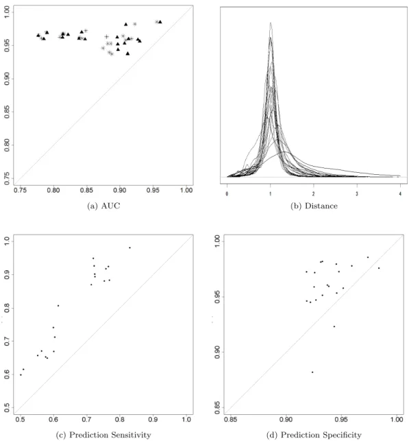
Second, the area under the ROC curve (AUC) was computed. This was accomplished by plug-ging in the posterior means of the model parameters and the latent positions into the observation equations (2.3) and (2.4), and then comparing these with the simulated dataY1:T. Hence this can be considered as a measure of how well the model fits the data. For each simulation, the directed graphs were also converted to undirected graphs by letting yijt = max{yijt, yjit} in order that we might apply the method of Sarkar and Moore (2005). The AUC values for both undirected and directed networks were then computed using the estimates from Sarkar and Moore’s method. We similarly computed the AUC values for the directed network using our method, and, again using those same estimates, computed the AUC values for the undirected network by using_P(_{yijt= 1} ∪ {yjit= 1}). These results are given in Figure 2.5a, where asterisks indicate the directed networks and triangles indicate undirected. We see that all our values are extremely high, implying that the model fits the data quite well, and also we see that our method uniformly outperformed that of Sarkar and Moore on both the directed and undirected networks.

Third, the pairwise distances from the estimated latent positions were compared to the pairwise distances from the true latent positions. That is, for each triple (i, j, t) we can look at _kXbit−

b

Xjtk/kXit− Xjtk, giving usT n(n−1)/2 such ratios for each simulation. Figure 2.5b gives, for each of the twenty simulations, a smoothed curve of the distribution of these ratios. Notice that all these distributions are narrow and centered around 1, implying that the latent positions from the posterior means are close to the truth.

Fourth, the capability of predicting YT+1 was evaluated. To this end one could simulate a new XT+1 from (2.2) and subsequently simulate a newYT+1from (2.3) and (2.4), and then compare the predicted edges with these simulated edges. This would, however, introduce unnecessary variation inYT+1, possibly making good predictions seem bad, or vice versa. Hence we used P(YT+1|XT+1=

E(XT+1|XT,ψ),ψ) as the “true” probabilities at time T + 1. We first wanted to make sure that the more sophisticated prediction method worked better than plugging the posterior means into the observation equations. Hence we compared the sum of squared differences between the true probabilities and the predicted probabilities given by (2.23) to the sum of squared differences between the true probabilities and the probabilities obtained by plugging in the posterior means into (2.3) and (2.4). Specifically, we looked at

(31)

of 0.9725 (0.8679). This implies that better prediction estimates can be obtained when we do not condition on the model parameters. We then letyij(T+1)= 1 if the true probability was greater than 1/2. Using the newYT+1 we computed the AUC for the predicted probabilities, leading to a mean (sd) over the simulations of 0.9546 (0.04003). Finally, making hard predictions of 1 if the predicted probability was greater than 1/2 we computed the sensitivity and specificity. We also compared these values to simply usingYT to make hard predictions. The results are given in Figures 2.5c and 2.5d, where the vertical axis corresponds to our predictions and the horizontal axis corresponds to YT. Clearly by using our prediction method we obtain much better sensitivity, and though the specificity is much more comparable, our method still does better in all but three of the 20 simulations.

For those ten cases where nodal influence was part of the simulation, we computed the sensitivity of detecting nodal influence on those nodes which were in truth influenced, and in all 20 simulations we computed the specificity of not detecting influence on those nodes which were in truth not influenced. The mean (sd) sensitivity and specificity for the ten simulations with nodal influence were 0.952 (0.0316) and 0.832 (0.129). The mean (sd) specificity for the ten simulations without nodal influence was 0.868 (0.116). We see from this that the Bayesian estimation does a very good job at detecting nodal influence without giving many false positives when no such influence exists.

Sensible priors have been outlined in Section 2.2.1 for all model parameters except σ2_{. It is} important then to determine the sensitivity of the MCMC algorithm to the values ofθσandφσ. To this end we reran the above simulations where the shape and scale parameters ofπ(σ2) were drawn from a uniform distribution ranging from 3 to 15 for the shape parameter and from 0.01 to 2 for the scale parameter. The AUC for rerunning these 20 simulations in this fashion yielded very high AUC values, ranging from 0.9407 to 0.9858, averaging 0.9621. Thus it appears that the estimation is quite robust to the hyperparameters for the prior ofσ2_.

In addition to the simulations described above, five larger data sets were simulated wheren= 500 and T = 10. Estimation was performed both using and not using the approximations outlined in Section 2.2.3, letting n0 = 100, and the AUC was computed to evaluate model fit. Simulations were analyzed on a UNIX machine with a 2.40 GHz processor. The mean (sd) time to perform the MCMC analysis with 50,000 iterations using the approximation was, in minutes, 716 (24), and to perform the MCMC with 50,000 iterations not using the approximation was, in minutes, 2281

(32)

Thus by using the approximations of Section 2.2.3 there is a drastic decrease in computational time with very little loss in model fit.

(a) AUC (b) Distance

(c) Prediction Sensitivity (d) Prediction Specificity

Figure 2.5: Results for 20 simulations. (a) AUC using Sarkar and Moore’s method (horizontal axis) and our method (vertical axis) on both undirected (triangles) and directed (asterisks) networks; (b) Distribution of pairwise distance ratios, comparing estimated latent positions with true latent positions; (c)-(d) Sensitivity and Specificity for predicting edges at timeT + 1, using YT to make predictions (horizontal axis) and our method of prediction (vertical axis).

(33)

● ● ● ● ● ● ● ● ● ● ● ● ● ● ● ● ● ● ● ● ● ● ● ● ● 1 2 3 4 5 6 7 8 9 10 11 12 13 14 15 16 17 18 19 20 21 22 23 24 25 ● ● ● ● ● ● ● ● ● ● ● _● ● ● ● ● ● ● ● ● ● ● ● ● ● 1 2 3 4 5 6 7 8 9 10 11 ₁₂ 13 14 15 16 17 18 19 20 21 22 23 24 25 ● ● ● ● ● ● ● ● ● ● ● ● ● ● ● ● ● ● ● ● ● ● ● ● ● 1 2 3 4 5 6 7 8 9 10 11 12 13 14 15 16 17 18 19 20 21 22 23 24 25 ● ● ● ● ● ● ● ● ● ● ● ● ● ● ● ● ● ● ● ● ● ● ● ● ● 1 2 3 4 5 6 7 8 9 10 11 12 13 14 15 16 17 18 19 20 21 22 23 24 25

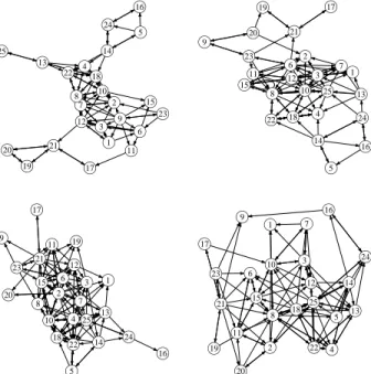
Figure 2.6: Graphs of Dutch classroom data at, from left to right and top to bottom, times 1, 2, 3, and 4.

2.7 Real Data Analyses

2.7.1 Dutch Classroom Data

Knecht (2008) conducted a longitudinal study in which students aged 11 to 13 years in a Dutch class were surveyed over four time points, yielding four asymmetric adjacency matrices where the (i, j)th _{entry denotes whether student} _i _{claims student}_j _{as a friend. Figure 2.6 shows the graphs} from these adjacency matrices. Demographic and behavioral data were also collected on these individuals. Twenty six students were recorded, although one student left the class before the study was completed; this student was left out of the analysis. Missing edges exist in the data due to some students not being present during a survey. This was dealt with as previously described in Section 2.3.

A burn-in of 15,000 iterations was removed, leaving a chain of length 85,000. We compared our method with that found in Sarkar and Moore (2005) by AUC values. Our method yielded an AUC value of 0.917 vs. 0.8456 from Sarkar and Moore’s method.

Statistical models and inference for dynamic networks