Original Paper
Hum Hered 2016;82:1–15 DOI: 10.1159/000475465
Efficient Maximum Likelihood Estimation
for Pedigree Data with the Sum-Product
Algorithm
Alexander Engelhardt
a
Anna Rieger
a
Achim Tresch
c
Ulrich Mansmann
a, b
a Institute for Medical Informatics, Biometry and Epidemiology and b Institute for Statistics, Ludwig Maximilian University, Munich , and c Institute for Medical Statistics and Computational Biology, University Clinic Cologne, Cologne , Germany
time-efficient tool for statistical inference in biomedical event data with latent variables that opens the door for ad-vanced analyses of pedigree data. © 2017 S. Karger AG, Basel
Introduction
Colorectal cancer (CRC) is one of the most prevalent
cancer diseases in Europe and the United States
[1]
, with
men having a younger average age at diagnosis
[2]
. For a
small proportion of CRC cases, genetic predispositions
are known
[3]
. Interestingly, an additional 15–20% of
CRC cases occur in familial clusters
[4]
. Within these
clusters, family members show a higher risk of
contract-ing CRC
[5]
. The cause for these clusters is unknown but
assumed to be a risk factor which may be of genetic or
environmental origin.
Since cancer develops earlier in these high-risk families,
it is of interest to identify them in advance. Subsequently,
health insurances can allow members of high-risk families
to join screening programs at an earlier age. In this paper,
we therefore develop an efficient risk calculator for CRC,
i.e., a method for clinicians to assess the familial risk for a
specific family based on the family’s CRC history.
Keywords
Colorectal cancer · Personalized medicine · Cancer risk prediction · Pedigrees · EM algorithm · Factor graphs · Sum-product algorithm
Abstract
Objective: We analyze data sets consisting of pedigrees with age at onset of colorectal cancer (CRC) as phenotype. The occurrence of familial clusters of CRC suggests the existence of a latent, inheritable risk factor. We aimed to compute the probability of a family possessing this risk factor as well as the hazard rate increase for these risk factor carriers. Due to the inheritability of this risk factor, the estimation necessi-tates a costly marginalization of the likelihood. Methods: We propose an improved EM algorithm by applying factor graphs and the sum-product algorithm in the E-step. This reduces the computational complexity from exponential to linear in the number of family members. Results: Our algo-rithm is as precise as a direct likelihood maximization in a simulation study and a real family study on CRC risk. For 250 simulated families of size 19 and 21, the runtime of our algo-rithm is faster by a factor of 4 and 29, respectively. On the largest family (23 members) in the real data, our algorithm is 6 times faster. Conclusion: We introduce a flexible and
Received: December 13, 2016 Accepted: April 1, 2017 Published online: July 21, 2017
To do this, we look at data consisting of a set of
pedi-grees, where each person has an inheritable latent
vari-able, the risk factor, that influences its phenotype, the age
at CRC diagnosis. Assuming an inheritance model and a
penetrance model, we aim to estimate 2 parameters: the a
priori probability
p
1
for a founder to carry the risk factor,
and the penetrance
α
(i.e., the multiplicative increase of
the hazard rate of an individual that carries the risk
fac-tor).
A closely related subject is
complex segregation
analy-sis
. Segregation analysis evaluates whether pedigree data
of affected and unaffected offspring agree with a
mende-lian transmission mode and perform hypothesis tests for
different models of inheritance
[6]
. Complex segregation
analysis can go one step further and work with pedigrees
of arbitrary structure instead of nuclear families and
quantitative traits as well as qualitative traits
[7]
. We
per-form a kind of segregation analysis but do not test for a
specific genetic model. In accordance with the argument
in Houle et al.
[8]
, we employ a phenotype-based
ap-proach to study a generic inheritance mechanism,
be-cause the details of genetic causation of CRC are still
un-known and complex, and the assumptions of a
genotype-based approach may not hold true.
This problem has been approached in previous work
of our group
[9]
. Since the latent variable is unknown but
influences the likelihood, a straightforward estimation
procedure has to marginalize the likelihood respective to
them. The inheritability of this latent variable means that
observations within a family are dependent, and the
mar-ginalization cannot happen on the level of a single person,
but over a whole family. Since each latent variable can
as-sume 1 of 2 values (risk factor present: yes/no), the
com-plexity of computing this sum is
(2
D), where
D
is the
number of family members.
The runtime of this straightforward optimization over
the marginalized likelihood is still reasonable when no
family has an excessive number of members. However,
the number of possible risk constellations within a family
grows 2-fold with each new family member. As soon as
even 1 family is sufficiently large, the marginalization
quickly becomes unfeasible. In these situations, an
alter-native approach is needed.
The new aspect in this paper is the implementation of
an expectation-maximization (EM) algorithm for
situa-tions when some families are too large for the
marginal-ization procedure. The E-step is nontrivial because the
latent variables within a pedigree are dependent, and a
straightforward calculation of the marginal posteriors
would again be of exponential runtime. For a linear
de-pendency structure (such as in a Hidden Markov Model),
the Baum-Welch algorithm
[10]
is an efficient method for
solving the E-step. In our problem, the data instead show
dependency in a tree structure. This dependency
struc-ture necessitates using the sum-product algorithm
[11]
to
obtain the marginalized posterior probabilities for the
la-tent variables in the E-step. A similar approach for the
marginalization over hidden variables has been proposed
and implemented by Failmezger et al.
[12]
, yet in the
completely different context of single cell time lapse
im-age analysis.
We show that the runtime of our EM algorithm is
lin-ear instead of exponential in terms of the pedigree size.
We also executed a simulation study to show that our
al-gorithm correctly recovers the specified parameters.
Fi-nally, we demonstrate the runtime improvement of our
algorithm on a real data set: a family study of CRC cases
in Upper Bavaria.
Methods
Nomenclature
The data set is composed of families which are represented as pedigrees ( Fig. 1 a). We call individuals at the top of the pedigree (i.e., with unspecified parents) founder nodes and all other persons
nonfounders . Individuals without any offspring (i.e., at the bottom of the pedigree) are called final individuals.
We denote by t i the chronological age in years at clinical onset
of CRC for each person i = 1, …, n , if the corresponding censoring indicator c i equals 1, and the age at censoring if c i = 0. The gender
of an observation is denoted by m i , which is 1 for males and 0 for
females. The observed data for 1 person is thus x i = ( t i , c i , m i ).
Each person also has a latent variable z i which equals 1 if this
person is a risk carrier and 0 if not. We use ♂ i and ♀ i to denote the
position (i.e., the value of i ) of the father and mother of person i . For example, if we have a risk status z i for a nonfounder i , his
fa-ther’s risk status is z ♂ i . We denote the set of all i that are founder
nodes by F . The complete data vectors for all patients are called x and z , respectively.
Penetrance Model
For persons where z i = 1, we assume an elevated relative risk of
developing CRC, which manifests itself through a hazard rate in-creased by a multiplicative factor α , the penetrance [5] . This pa-rameter is unknown and will be estimated.
We assume a Weibull distribution for t i , because it is a
paramet-ric distribution which fits observed CRC incidence curves quite well. The Weibull hazard rate is given by h ( t ) = kλ k t k –1 , with the parameters k > 0 and λ > 0. In our relative risk model, we multiply the hazard rate by α if z i = 1 and, additionally, by β if m i = 1. These
factors model the increased relative risk for risk carriers and males, respectively. Our hazard rate for an event (i.e., diagnosis of CRC) is then
The survival function is defined by S ( t ) = exp(– ∫ t
0 h ( u )d u ). With the additional relative risk factors, this becomes
S ( t i ) = exp(–( t i λ ) k α z i β m i ).
The density for 1 observation i is composed of the product of the survival function and (for uncensored observations) the hazard rate:
f(t i | z i ) = h ( t i ) ci · S ( t i ).
The observations x i are conditionally independent given z i , and the
density of the whole data f ( x | z , θ ) can be split up into a product of
individual densities: f ( x | z , θ ) = Π i f ( x i | z i , θ ).
Heritage Model
The founder prevalence , i.e., the a priori probability P( Z i = 1)
for a founder node to carry the risk factor, is called p 1 . This param-eter will be estimated. The probability for a nonfounder to be a risk carrier is dependent on its parents’ risk statuses and the inheritance probability p H . Our model does not allow for spontaneous
muta-tions to risk carrier. If any one of both parents passes down a risk factor z ♂ i = 1 or z ♀ i = 1 with the probability p H , then the
probabil-ity for the offspring to be a risk carrier is p ∼ i = P( Z i = 1 | z ♂i , z ♀ i ) = p H z ♂i + p H z ♀ i – pH 2 z ♂ i z ♀ i . (1)
We denote P( Z i = 1 | z ♂i , z ♀ i ) for nonfounders by p ∼ i to emphasize
the distinction from p 1 for founders.
A sensitivity analysis found that varying the value of p H has a
negligible effect on the final parameter estimates [9] , and thus we chose p H = 0.5 for all our analyses.
Given a predefined inheritance probability p H and a founder
prevalence p 1 , the probability for a risk vector Z for the entire da-taset becomes 1 1 1 1 1 1 P( ) P( ) P( (1 ) ( ) 1 ) i i i i i i i F i F z z z z i F i i F i z z z z p p p , | z p ¸ ¸
̓ ͂ LikelihoodsAll Weibull parameters ( k , λ ) as well as the inheritance proba-bility p H and the risk increase for males ( β ) are assumed to be
known. We set k = 4 and λ = 0.0058 according to Rieger and Mansmann [9] , β = 2 according to Kolligs et al. [2] , and p H = 0.5.
The complete likelihood, where both x and z are observed, is then
L ( θ ; x , z ) = f ( x , z ) = f ( x | z )P( z ). (2)
The 2 factors f ( x | z ) and P( z ) were defined in the penetrance
mod-el and the inheritance modmod-el, respectivmod-ely. The parameter vector in our model is θ = ( p 1 , α ).
The complete log-likelihood becomes (derivation in Appen-dix A1)
1 1 1 , const | | log 1 log i i. i i i F i F n k z m i i i i l ; x z z p F z p c z t ␣ ␣  ¬ ¬
®
®
⫹ ⫹ ⫺ ⫺ ⫹ ⫺ log (3) We marginalize the nonreduced form of the complete likelihood to obtain the incomplete likelihood L ( θ ; x ) [ 13 , Equation 1.5]:; ; ,
z
L x
L x z . (4)To estimate the parameters p 1 and α , one could use a Nelder-Mead optimization [14] on the marginalized likelihood L ( θ ; x ). How-ever, for a family of size D , the sum over all z has 2 D elements. Even
when splitting the sum up across all families (Appendix A3), the number of summands grows exponentially with increasing fam-ily size D . Thus, for large families, the computation of the margin-alization within the likelihood evaluation quickly becomes unfea-sible.
The EM Algorithm
A common approach for finding maximum likelihood esti-mates in the presence of latent variables is to make use of the EM algorithm. Resources on the EM algorithm are plentiful, including
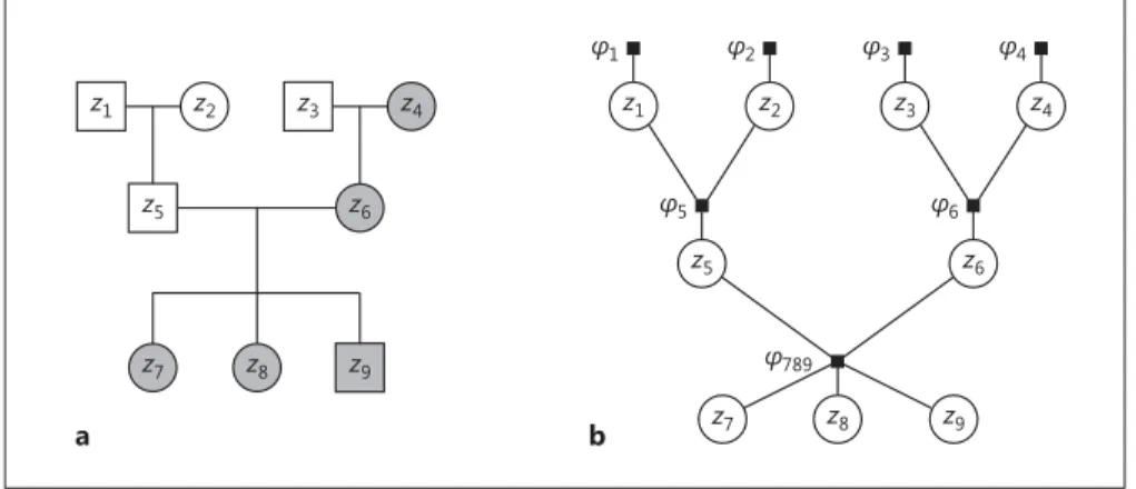
Ĵ1 z1 Ĵ2 Ĵ789 z2 Ĵ5 Ĵ3 z3 Ĵ4 z4 Ĵ6 z5 z6 z7 z8 z9 b a z1 z2 z5 z9 z7 z3 z4 z6 z8
Fig. 1. A pedigree and its corresponding factor graph. a A sample pedigree of a family with 9 members. Squares denote males, circles females. A couple (a connected circle and square in the same row) gives rise to a set of children (the nodes connected to this couple in the row below). Persons shaded in grey are risk carriers. The 4 grandparents in the top row are the founder nodes in this family,
the other 5 persons are nonfounders . b A factor graph visualizing the factorization of g ( z ) = f ( x , z ) (Equation 2) for the family from Figure 1a. Circles represent variable nodes, and filled squares rep-resent factor nodes (i.e., local functions). The edges show which variables are arguments to which factor. For example, the factor φ 6 has 3 arguments: φ 6 ( z 3 , z 4 , z 6 ).
a short tutorial [15] , the seminal paper by Dempster et al. [16] , and an entire book [17] devoted to the subject.
In short, the EM algorithm proceeds in a loop over 2 steps: in the E-step , one calculates the expected log-likelihood over the la-tent variables Z , given the observed data and the current parameter estimates. This problem reduces to computing complete-data suf-ficient statistics [16] . In the subsequent M-step , one then updates the estimates of the parameters, given the new expected sufficient statistics from the E-step.
As a convergence criterion, frequent choices include the size of the relative change of either the log-likelihood or the parameter estimates [18] .
We use the size of the relative change of the parameter esti-mates for α and p 1 as a stopping criterion. This criterion is more conservative than using the log-likelihood [18] , and we are on the safe side by letting the algorithm run a bit longer than it would have to.
To compute the expected log-likelihood Q ( θ ; θ ( t ) ), we introduce the membership probabilities [ 17 , p. 43] T ( i t ) , i.e., the probability for one person’s risk status Z i , given the whole observed data x
(deriva-tion available in Appendix A2):
| , | , E E P 1| , P | , . t t i t i Z x i i Z x t i t i z T Z Z Z x z z x
(5)Here, the summation is over all admissible combinations of z i
(i.e., P( z ) > 0 and z i = 1). The condition on the entire observed
data x and the summation over all z will conveniently reduce to a condition on and summation of only the respective family’s data x and z (Appendix A3). The target function Q becomes (cf. Equation 3)
| , 1 1 1 ; ,
const log log 1 1
log 1 . t i t Z x t t i i i F i F n k m t t t i i i i i i Q ; E l x Z p T p T T c t T T ␣  ␣ ¯ ¡¢ °± ¬ ¬ ® ®
⫹ ⫹ ⫺ ⫺ ⫺ ⫹ ⫺ (6) The M-StepFor the M-step, we maximize Q ( θ ; θ ( t ) ) respective to α and p 1 to obtain the new parameter estimates for iteration t + 1. Once the values of all T ( i t ) are known, the maximization of Q with respect to p 1 and α is straightforward and has a closed form solution:
1 1 1 . i n t i i i t k n t m i i i c T T t
␣  ⫹ (7) 1 1 . | | t t i FTi p F
⫹ (8) The E-StepIt follows from Equations 6–8 that, as in the “standard” exam-ples of the EM algorithm, the E-step conveniently reduces to com-puting the complete-data sufficient statistics T ( i t ) . The reason for
this simplification is the fact that the log-likelihood is linear in the latent data Z . Computing Q ( θ ; θ ( t ) ) thus simplifies to replacing each occurring Z i by its conditional expectation T ( i t ) . The M-step then
uses these “imputed” values of the latent data Z for the updated parameter estimates.
Marginalization of the Joint Density
In our setting, the difficulty in computing T ( i t ) is that the prob-ability for the risk status of 1 family member Z i is conditioned on
the observed data x of the entire family (Appendix A3). To com-pute these values, we could marginalize over all risk vectors z where z i = 1, i.e., T (i t ) ∑ r P( Z = r | x , θ ( t ) ), where r is a valid risk
vec-tor (i.e., with P( Z = r ) > 0 and with z i = 1). However, this requires
the same exponential runtime as in a Nelder-Mead optimiza-tion.
Alternatively, a pedigree can be represented as a Bayesian net-work [19, 20] , also known as a causal probabilistic network, which in turn can be converted into a factor graph [11] . This representa-tion is advantageous because it allows the efficient computarepresenta-tion of marginals via the sum-product algorithm.
The sum-product algorithm [11] , also known as the belief propagation algorithm, computes marginalizations of the form of
T ( i t ) in linear runtime [ 21 , p. 290]. It does this by representing a complex “global” function g ( z ) – here, f ( x, z | θ ( t ) ) – as a factor
graph, i.e., a product of multiple “local” functions, Π j φ j , each
de-pending on only a subset of the arguments in g ( z ).
The sum-product algorithm then exploits this structure to ef-ficiently compute marginalizations of g ( z ) – here, we marginalize the joint density to obtain f ( z i , x | θ ( t ) ). By dividing this joint
den-sity through f ( x ) = f ( Z i = 1, x | θ ( t ) ) + f ( Z i = 0, x | θ ( t ) ), we ultimately
obtain T ( i t ) = P( Z
i = 1 | x , θ ( t ) ), which was our actual goal.
Factor Graphs
Factor graphs were first introduced by Kschischang et al. [11] to represent factorizations of multivariate functions.
The factor graph in Figure 1 b encodes the joint density g ( z ) =
f ( z , x ) of the family from Figure 1 a as the product of 7 factors φ j :
g ( z ) = φ 1 ( z1 ) · φ 2 ( z 2 ) · φ 3 ( z3 ) · φ 4 ( z 4 ) · φ 5 ( z1 , z 2 , z 5 )
· φ 6 ( z3 , z 4 , z 6 ) · φ 789 ( z 5 , z 6 , z 7 , z 8 , z 9 ). (9)
The factors are defined as ( ) ( ) (P ) J J J J j j j j J z ,z ,z f x z| z | z ,z ,
͂ K ̓ ̓ ͂where J is the set of all children with the same parents, which are denoted by z ♂ J , and z ♀J . If φ J is a factor for a founder node, then z ♂ J
and z ♀ J are defined as an empty set and the respective probability
P( z j ) is unconditioned. The exemplary factors for Equation 9 are
available in Appendix A4.
The factor φ 789 ( Fig. 1 b) cannot be split up into 3 factors be-cause the graph edges would then form a cycle , which is not al-lowed, or would necessitate a costly loopy belief propagation pro-cedure [11, 22] . Instead, we implement a clustering procedure [11] and group the respective densities into 1 factor per set of parents.
The Sum-Product Algorithm
Having set up a factor graph for each family, we then apply the sum-product algorithm to compute marginalizations of f ( z , x ) at each variable node z i , i.e., f ( z i , x ). In our setting, we restrict
our-selves to family trees , i.e., we do not allow for consanguineous mar-riages (see Fig. 2 of Goddard et al. [23] for a counterexample), which would again lead to cycles in the corresponding factor graph.
Let μ z → φ ( z ) denote the message sent from a variable node z to
a factor node φ , and let μ φ → z ( z ) denote the message sent from a
factor node φ to a variable node z . Furthermore, let n ( v ) denote the set of neighboring nodes of a (factor or variable) node v .
We then define the messages from a variable node to a factor node, and from a factor node to a variable node, as follows [11] :
\ ^
\ ^ \ ^ \ \ , z h z h n z z y z y n z z z z Z y l l l l ¬ ®
where Z φ is the set of arguments of the factor φ . If h ∈ n ( z )\{ φ } =
{}, e.g., at a variable node of a final individual (the grandchildren
z 7 , z 8 , and z 9 in Figure 1 b), the product is defined as 1. The expres-sion ∑ ∼ { z } is adapted from Kschischang et al. [11] and denotes the not-sum (i.e., the sum over all variables except z ).
Finally, the marginalization, or termination step , computes the value of g i ( z i ) = ∑ ∼{ z i } g ( z ) as the product of all incoming messages on a variable node z i . The marginalized g i ( z i ) are equal to f ( z i , x | θ ( t ) ), i.e., proportional to the desired outputs T
i
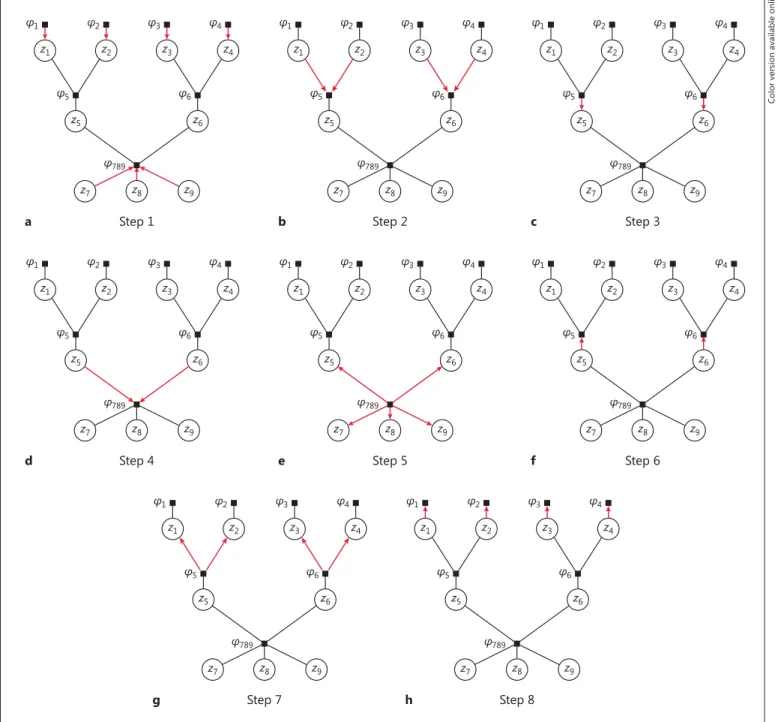
( t ) from the E-step in the EM algorithm. We show some example messages and mar-ginalizations of the sum-product algorithm in the following sec-tion. We provide a detailed computation and illustration of all pos-sible messages in Appendix A5 and Figure 2 and give a summa-rized proof of correct convergence of our algorithm in Appendix A6.
We implemented a sum-product algorithm for computing the marginals of an arbitrary pedigree in R [24] and made it available on GitHub (all scripts are available on GitHub, http://github.com/ AlexEngelhardt/sumproduct). The code creates 1 factor graph per family, and therein 1 factor node per founder, which contains
φ i ( z i ) = f ( x i | z i ) · P( z i ). Furthermore, we create 1 factor per set of
parents, which contains the product of all densities of all children (but not the parents):
φ j (Z j ) = Π i ∈ K j f ( x i | z i ) · P( z i | z ♂ i , z ♀ i ),
where Z j represents all variables within the factor (parents and
children), and K j is the set of children variables connected to φ j .
Messages from a “large” factor containing parents and many children will be summed over all neighboring variable nodes ex-cept the destination variable node. By iteratively exploiting the dis-tributive law, this sum can be efficiently broken down from expo-nential to linear runtime. For an example based on Figure 1 b, see Appendix A7.
Example Messages and Marginalizations of the Sum-Product Algorithm
We illustrate the sum-product algorithm by calculating 2 ex-ample messages and 1 exex-ample marginalization from the pedigree of Figure 1 b.
Firstly, the message μ z 6 → φ 789 ( z 6 ) from the variable node z 6 to
the factor node φ 789 equals
μ z 6 → φ 789 ( z 6 ) μ φ 6 → z 6 ( z 6 ).
Secondly, the message μ φ 5 → z 2 ( z 2 ) from the factor node φ 5 to the
variable node z 2 equals
5 2 1 5 5 5 1 5 2 5 1, 2, 5 1 5 . z z z z z z z z z z z l
. l lLastly, we compute the example marginalization at the variable node z 5 as g 5 ( z 5 ) = f ( z 5 , x | θ ( t ) ) = μ φ 5 → z 5 ( z 5 ) · μ φ 789 → z 5 ( z5). Then,
5 5 789 5 5 5 789 5 5 5 789 5 5 5 5 5 5 P 1| , 1, | 0, | 1, | 1 1 . 0 0 1 1 t t t t t z z z z z z T Z x f z x f z x f z x l l l l l l ⫹ . . .
This shows that the desired values T ( i t ) from the E-step are imme-diately obtained as soon as all possible messages are computed.
Appendix A5 and Figure 2 show the detailed derivation of all remaining messages.
Convergence of the EM Algorithm
A common drawback among many estimation algorithms is the danger of converging into a local maximum. This also applies to the EM algorithm. However, we will show that the marginal likelihood function (Equation 4) is concave and thus the EM algo-rithm will always converge to the global maximum of the margin-al likelihood, irrespective of the initimargin-al parameter choice.
A twice differentiable function is concave if its Hessian matrix is negative semidefinite. We first show that the Hessian of the complete log-likelihood function (Equation 3) is negative semi-definite. Since the variables α and p 1 are separated, ∂ 2 / ∂ α ∂ p 1 l ( θ ; x , z ) = 0, and consequently the Hessian is a diagonal matrix. It suf-fices to show that both its diagonal entries are zero or negative. We obtain
2 2 2 2 1 1 1 | | ; , . 1 i i i Fz F i Fz l x z p p p s s
⫺
⫺ ⫺ ⫺ (10) 2 2 2 1 ; , . n i i i c z l x z ␣ ␣ s s ⫺
(11)Note that in Equation 10, ∑ z i ≤ | F |; hence, both terms on the
right-hand side of this equation are negative or zero. This proves that the complete log-likelihood is concave. Since the exponential is strictly monotonically increasing and l ( θ ; x , z ) is strictly con-cave, it follows that L ( θ ; x , z ) = exp( l ( θ ; x , z )) has only 1 unique local and hence global maximum [25] . Finally, the marginal log-likelihood, as the sum ∑ z l ( θ ; x , z ) of concave functions, is also
concave. This means that simpler but faster optimization algo-rithms such as Nelder-Mead can be used for our model, and there is no need for more complex algorithms such as stochastic or constrained optimizers (e.g., L-BFGS-B [26] or simulated anneal-ing [27] ).
Ĵ1 z1 Ĵ2 Ĵ789 z2 Ĵ5 Ĵ3 z3 Ĵ4 z4 Ĵ6 z5 z6 z7 z8 z9 Ĵ1 z1 Ĵ2 Ĵ789 z2 Ĵ5 Ĵ3 z3 Ĵ4 z4 Ĵ6 z5 z6 z7 z8 z9 Ĵ1 z1 Ĵ2 Ĵ789 z2 Ĵ5 Ĵ3 z3 Ĵ4 z4 Ĵ6 z5 z6 z7 z8 z9
a Step 1 b Step 2 c Step 3
Ĵ1 z1 Ĵ2 Ĵ789 z2 Ĵ5 Ĵ3 z3 Ĵ4 z4 Ĵ6 z5 z6 z7 z8 z9 Ĵ1 z1 Ĵ2 Ĵ789 z2 Ĵ5 Ĵ3 z3 Ĵ4 z4 Ĵ6 z5 z6 z7 z8 z9 Ĵ1 z1 Ĵ2 Ĵ789 z2 Ĵ5 Ĵ3 z3 Ĵ4 z4 Ĵ6 z5 z6 z7 z8 z9
d Step 4 e Step 5 f Step 6
Ĵ1 z1 Ĵ2 Ĵ789 z2 Ĵ5 Ĵ3 z3 Ĵ4 z4 Ĵ6 z5 z6 z7 z8 z9 Ĵ1 z1 Ĵ2 Ĵ789 z2 Ĵ5 Ĵ3 z3 Ĵ4 z4 Ĵ6 z5 z6 z7 z8 z9 g Step 7 h Step 8
Fig. 2. Message passing during the sum-product algorithm. The messages are computed iteratively. Once all but 1 incoming messages are calculated for a given node, a message is calculated and sent across the remaining edge. Note that by Kschischang et al. [11] , the actual order in which the messages are calculated is irrelevant for the result.
Application: Estimating the Probability of Being a Risk Family
Applying the sum-product algorithm directly implies a straightforward method to compute the probability of being a risk family.
After we have estimated p 1 and α , we can estimate the prob-ability that this family carries the risk factor for a new pedigree (or a pedigree from the original study, i.e., the training data). We define a risk family as a family in which at least 1 member is car-rying the risk factor (i.e., z i = 1 for at least one i ). This is exactly
1 minus the probability that no family member carries the risk factor. If we restrict the data x and Z to just the family in ques-tion, and define the event R as “The family is a risk family,” we can then compute
P( R ) = 1 – P( Z = 0 | x , θˆ ) (12) 1 P 0 | ,
. i i F ˆ Z x ⫺
(13) 1 1 t . i i F T ⫺
⫺ (14)The step from Equation 12 to Equation 13 is possible because the probability that no family member carries the risk factor equals the probability that no founder carries the risk factor, since the former is true if and only if the latter is true. Then, we can split up the joint probability that no founder carries the risk factor into the indi-vidual probabilities P( Z i = 0 | x , θˆ ). This step is possible because we
only consider the founders, and their risk probabilities are inde-pendent of any other z i .
Since P( Z i = 0 | x , θˆ ) equals 1 – T
i
( t ) by definition (Equation 5), we can simply run the E-step of the EM algorithm once on the new family to obtain these values. We then multiply over only those T ( i t ) where i ∈ F and obtain P( R ), an estimator for the familial CRC risk.
Results
Simulation Study
We performed an in silico experiment by simulating
data sets with a given
p
H
,
p
1
, and
α
and with a varying
number of families (
N
) and pedigree size (
D
). The risk
status
z
i
for each founder was randomly sampled with the
probability P(
z
i
= 1) =
p
1
, the statuses for all nonfounders
were sampled according to Equation 1. The age at onset
of CRC was then simulated according to a Weibull
distri-bution with the best fitting parameters according to
Rieg-er and Mansmann
[9]
,
λ
= 0.0058 and
k
= 4, and a risk
increase for males of
β
= 2:
f ( t i | z i ) = h ( t i ) · S ( t i ) = [ k λ k tki –1 α z i β m i ] · exp(–( t i λ ) k α z i β m i ).
We then simulated a censoring age
u
i
from the following
Gaussian distribution:
u
i
∼
(125, 100). The rather
opti-mistic mean censoring age of 125 years was chosen to keep
the ratio of censored subjects below 66%, since a higher
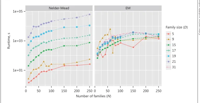
Nelder-Mead EM ŃŃ ŃŃ ŃŃ Ń Ń Ń Ń Ń Ń Ń Ń Ń ŃŃ Ń Ń Ń Ń ŃŃ Ń Ń Ń 1e+01 1e+03 1e+05 0 50 100 150 200 250 0 50 100 150 200 250 Number of families (N) Runtime, s Family size (D) Ń 5 9 15 17 19 21 31
Color version available online
Fig. 3. Runtime comparison of Nelder-Mead optimization (left) and the EM algorithm (right). Shown is the run-time in seconds on the y axis (log scale) versus the number of families on the x axis. The effect of an increasing family size D is negligible with the EM algorithm, but exponential with the Nelder-Mead optimization. For the largest families of D = 31, only the EM algorithm could be run in a feasible time. The Nelder-Mead optimization would have taken around 2.7 years.
censoring rate would just necessitate a larger simulated data
set to reach the same stability. Each subject’s censoring
in-dicator
c
i
was then set to 1 if
t
i
<
u
i
and 0 otherwise. A value
of 0 therefore indicates a censored observation. If a subject
is censored,
t
i
was replaced by
u
i
, the age at censoring.
Runtime Improvement
We simulated data sets with different pedigree sizes to
investigate the threshold pedigree size from which the
EM algorithm is faster than a Nelder-Mead optimization.
Figure 3 and Table 1 show the runtime of the
Nelder-Mead optimization versus the EM algorithm for different
data sizes and pedigree sizes. The pedigrees used were:
•
D
= 5: two parents with 3 children
•
D
= 9: four grandparents, 2 parents, 3 children ( Fig. 1 a)
•
D
= 15: four generations with only 1 final individual
•
D
= 17: the same pedigree as for
D
= 15, with 1
addi-tional parent pair for 1 founder
•
D
= 19: one more parent pair in the same generation
as for
D
= 17
•
D
= 21: one more parent pair in the same generation
as for
D
= 19
•
D
= 31: five generations with 1 final individual.
The results suggest that using the EM algorithm is
ad-vantageous as soon as
some
families in the data set are
large (more than around 17 members). For
D
= 31, we
ex-trapolated the runtime for the Nelder-Mead optimization
to about 2.7 years, according to a log-linear regression of
runtime against family size. This shows the dramatic
im-provement of using the EM algorithm as family sizes grow
larger. A more advanced EM algorithm could even split
the data into small and large pedigrees, and in the E-step
use the sum-product algorithm for the larger families, and
a “brute force” marginalization for smaller families.
Our Algorithm Recovers True Parameters
We simulated 100 replicated data sets of 500 families
of 9 persons as in Figure 1 a. In each replication, we chose
p
1
= 0.2 and
α
= 4 as the parameters and let the
Nelder-Mead optimization and the EM algorithm estimate the
parameters to investigate their level of agreement. Figure
4 shows scatterplots and Bland-Altman plots to compare
the 2 methods and finds a strong agreement between
them. Table 2 shows summary statistics on both methods’
parameter estimates in the 100 replications.
The Imputation of Noninformative Parents Works
When family members were randomly removed from
the data set after simulation, the imputation procedure
did not affect the results – both algorithms still converged
to the correct result after imputing took place. The
simu-lation and estimation were performed as in Figure 4 , but
20% of the family members were randomly removed
be-forehand. The preprocessing then performed an
imputa-tion of missing members. After our imputing procedure,
both algorithms still recover the true parameters (data
not shown; reproducible scripts available on GitHub).
Application: Estimating the Probability of Being a
Risk Family
We computed the posteriori probability of being a
CRC risk family for a simulated data set of 1,000 pedigrees
with 9 persons each, according to Equation 14. The
re-sulting ROC curve is shown in Figure 5 . The AUC of 0.74
shows that risk families can be identified with a
satisfy-ingly good rate.
Real Data
We applied our algorithm on a study exploring the
fa-milial CRC risk
[28]
. In this study, patients diagnosed
with CRC in the Munich region were recruited.
Table 1. Runtime ratio (Nelder-Mead over EM algorithm) over different family sizes D and different number of families N
Family sizes (D) 5 9 15 17 19 21 Number of families (N) 50 0.01 0.01 0.28 0.75 2.85 10.97 100 0.02 0.02 0.24 0.68 2.62 10.54 150 0.06 0.02 0.33 0.53 2.15 8.33 200 0.01 0.03 0.28 0.57 2.65 12.05 250 0.02 0.03 0.38 0.89 3.89 29.05
The EM algorithm is faster for pedigrees of size 19 and above, regardless of the number of families in the data set.
Table 2. Five-point summary and mean values for the parameter estimates of the Nelder-Mead optimization (N-M) and the EM al-gorithm, based on 100 simulated data sets
Mini-mum 1st quartile Median Mean 3rd quartile Maxi-mum pˆ1, N-M 0.1478 0.1740 0.1913 0.1929 0.2078 0.2864 pˆ1, EM 0.1476 0.1739 0.1912 0.1929 0.2078 0.2865 αˆ, N-M 2.888 4.036 4.347 4.310 4.656 5.297 αˆ, EM 2.890 4.037 4.345 4.310 4.660 5.287
quently, each of these
index patients
was given a
question-naire with a blank pedigree to fill out data about all known
relatives. With this obtained pedigree, the Munich
Can-cer Registry (MCR)
[29]
was consulted via an
anony-mized record-linkage procedure for any CRC diagnoses
of the index patient’s relatives
[30]
. The result was a
ped-igree of family data and CRC diagnoses per index patient.
The study was active from September 2012 until June
2014 and resulted in a data set of 611 families, of which
181 were just individuals (a “pedigree” with only 1
per-son).
In the real data set, pedigrees were not always recorded
in a directly useable manner. For observations with only
1 available parent, we imputed the missing parent as
non-informative (
c
i
= 0,
t
i
= 0 and with the appropriate gender
m
i
). In cases where a family consisted only of siblings, we
imputed both parents as noninformative observations to
indicate the relatedness of the siblings. The remaining
analysis was analogous to the in silico study described in
the Methods.
We estimated a prevalence of
p
1
= 0.901 and a risk
fac-tor increase of
α
= 5.723. We then performed a 100-fold
bootstrapping of families to obtain bootstrap standard
er-0.16 0.20 0.24 0.28 p1 convergence Nelder-Mead a b c d EM algorithm 3.0 3.5 4.0 4.5 5.0 į convergence Nelder-Mead EM algorithm 0.16 0.20 0.24 0.28 Bland-Altman plot of p1 Average Differ ence 3.0 3.5 4.0 4.5 5.0 Bland-Altman plot of į Average Differ ence 0e+00 4e–04 0.16 3.0 0.010 0 –0.010 3.5 4.0 4.5 5.0 0.20 0.24 0.28 –6e–04
Fig. 4. Convergence of 100 replications of simulating and estimating data sets. Each replication used random uniform distrib-uted starting values for θ = ( p 1 , α ). a , b The final parameter estimates for the Nelder-Mead optimization ( x axis) and the EM al-gorithm ( y axis). c , d Bland-Altman plots where the x axis shows the average of the parameter estimates of the 2 methods and the y axis shows their difference. Horizon-tal dashed lines are drawn at ±2 standard deviations of the difference. We see that both estimation methods agree with each other and converge close to the correct re-sult of p 1 = 0.2 and α = 4 regardless of start-ing values.
ROC curve for P(riskfam) AUC, 0.74
False positive rate
0 0.2 0.4 0.6 0.8 1.0 0 Tr ue positiv e rat e 0.2 0.4 0.6 0.8 1.0
Fig. 5. ROC curve for the probability of being a risk family, based on 1,000 simulated families with 9 persons (cf. Fig. 1 a).
rors. The values obtained were 0.0002 and 0.0229,
respec-tively.
The rather high a priori probability may stem from a
bias in the data set, since the collection procedure
prefer-ably selected patients and families that are already
ex-posed to risk. A more detailed discussion on the results is
given in Rieger and Mansmann
[9]
.
The data set contained 3 families with at least 20
mem-bers. For the largest family of 23 persons, using the EM
algorithm with the sum-product algorithm instead of a
Nelder-Mead optimization showed a reduction of the
runtime to 16%.
Discussion
Directly translating mathematical formulas into
com-puter code often results in a formally correct but slow
so-lution. In our case, a Nelder-Mead optimization would
need multiple evaluations of the marginalized likelihood,
which is unfeasible for larger families. An approach based
on
peeling
[31–33]
, however, could have been used to
re-duce the time for evaluating the likelihood. The
disadvan-tage of the Elston-Stewart peeling algorithm is that as
soon as the pedigree contains loops, its runtime increases
exponentially with the
cutset
(i.e., the number of
mem-bers that have to be considered jointly)
[13]
. The EM
al-gorithm coupled with the sum-product alal-gorithm can be
extended to pedigrees with loops by applying the “loopy
belief propagation” procedure
[11]
. Furthermore, peeling
algorithms need to find an optimal peeling order for each
pedigree, a problem that still has no gold standard
solu-tion today
[33]
. The sum-product algorithm, on the
oth-er hand, directly implies an efficient ordoth-er of computing
the messages, and thus elegantly circumvents this
prob-lem. Thompson and Shaw
[34]
showed that the EM
algo-rithm is a viable alternative to the peeling algoalgo-rithm in
polygenic models. Our approach differs from this in that
we skip the detection of responsible genes and instead
fo-cus on estimating a family’s probability of carrying an
(unspecified) CRC risk factor.
The EM algorithm with an approximative Monte
Car-lo implementation of the E-step has previously been used
on pedigrees for segregation analysis
[35]
. We saw that
the EM algorithm in our setting relied on a
marginaliza-tion over all possible risk vectors for each pedigree. This
problem of calculating marginal densities in hierarchical
data such as pedigrees has usually been tackled by Markov
Chain Monte Carlo (MCMC) simulations and related
sampling algorithms
[36, 37]
. Due to the random
sam-pling, these methods all yield only approximative
solu-tions and may take a long time to reach stable results. We
instead use the sum-product algorithm
[11]
within the
EM algorithm to solve the necessary marginalization in
the E-step in linear instead of exponential time. This
pro-vides a fast and exact solution and allows
maximum-like-lihood estimation with pedigrees of arbitrary size that,
furthermore, is not dependent on an arbitrarily chosen
number of MCMC simulations.
In contrast to complex segregation analysis, our
ap-proach is less specific. In particular, we only model an
unspecific risk “component,” not necessarily a gene or
multiple genes, which is passed down to offspring with a
certain predefined probability. We chose this
phenotype-based approach since the causes for familial occurrence
of CRC are currently unknown. Our generic model is
therefore not fully in line with mendelian transmission
models. Only under the assumption of an autosomal
dominant risk factor that is rare, so that an affected
indi-vidual can be assumed to have the genotype Aa instead of
AA, is a constant inheritance probability of
p
H
= 0.5
jus-tifiable. As an advantage, environmental risk factors such
as nutrition, lifestyle, or place of residence can be
mod-eled by choosing
p
H
= 1. If one wants to account for a
small probability of changing the place of residence, or a
probability for children to not adopt the parents’ lifestyle,
inheritance probabilities less than 1 can be used as well.
However, if a large enough data set were available, it
should also be possible to estimate
p
H
robustly enough.
One limitation of the real data set in this study is the
relatively small sample size. With around 600 families,
the data set was not large enough to obtain stable
esti-mates. However, since the focus of this study is
method-ological, the data set can still be used to show the runtime
improvement of our algorithm. The moderate gain in
speed in the application to the real data set can be
ex-plained by 2 facts. First, the multiplicative time constant
for the sum-product algorithm is larger than that for the
calculation of the marginal likelihood, since the message
passing needs more elementary operations than simple
summation over all possible configurations of the family
members (yet, as demonstrated in Figure 3 , this
disad-vantage is soon compensated by the exponential increase
in runtime of the Nelder-Mead method). Second, the
families in the real data set are mostly small (median size:
6 members), with the exception of a few larger families
(maximum size: 23). Thus, the full power of the EM
al-gorithm will unfold in applications where more, larger
families are investigated. The size of the families in such
studies is likely to grow in the future, with the
availabil-ity of more longitudinal data. Moreover, note that a
sin-gle, large family of more than, say, 25 members, will
pro-hibit the straightforward application of the
marginaliza-tion approach.
It should also be noted that for small families, the
lin-ear runtime of the sum-product algorithm is
slower
than
the exponential runtime of the marginalization, due to
the overhead in setting up the factor graph ( Fig. 3 ). In our
analysis, the sum-product algorithm had significant
ben-efits only as soon as a family consisted of more than 17
members.
It is possible to estimate further parameters in this
model, such as the shape parameter
k
. However, in our
case, these parameters were external epidemiological
in-formation, and thus already available from more robust
previous studies. Moreover, if additional parameters are
estimated, it should then be reevaluated whether the
Hes-sian matrix is still negative semidefinite (i.e., whether the
log-likelihood is still concave and unimodal).
Our algorithm can of course also be extended to other
models. For example, other penetrance models can be
used, such as a “time shift” model, where the hazard rate
is not multiplied by a factor
α
, but instead shifted
horizon-tally, by adding a “risk advancement” of a specific number
of years
[38]
. It is also possible to use different response
distributions besides a Weibull distribution. Furthermore,
it is possible to extend our method to model true
mende-lian transmission, either by having
Z
i
∈
{0, 1, 2} model the
number of affected alleles, or by specifying
two
latent
vari-ables,
Z
♂
∈
{0, 1} and
Z
♀
∈
{0, 1} per individual, 1 for each
allele. One would then need a transmission matrix to
spec-ify the probability of each possible outcome for offspring
given the statuses of both parents. Ghahramani
[39]
pro-vides a tutorial on how to extend a Bayesian network such
as a pedigree to deal with multiple latent variables.
When the number of possible genotypes (i.e., the
num-ber of possible values for
Z
i
) increases, both the EM
algo-rithm and the Nelder-Mead optimization suffer from
ex-ponential runtime increase. This is the case for example
when one works with multilocus genotypes. The runtime
of the EM algorithm is only linear respective to the
fam-ily size. However, since the genetic mechanism in our case
is unknown, a dichotomized latent variable served our
purpose well.
Faster algorithms such as the one presented in this
pa-per also open the door for new analyses that were
previ-ously unfeasible. With the sum-product algorithm, we can
now conduct large-scale simulation studies for power and
sample size determination and extract further
informa-tion such as bootstrap confidence intervals from the data.
Conclusion
In this paper, we developed an efficient algorithm for
maximum likelihood estimation where the observations
in the data are partially dependent. The rising size and
complexity of modern data sets make it necessary to
re-visit popular algorithms for data analysis and develop
im-provements in their efficiency. Here, we considered
clin-ical data in the form of pedigrees, where the presence of
latent and inheritable genetic risk factors greatly
compli-cated the analysis procedure. In our case, a standard
im-plementation of the EM algorithm results in a runtime
that is still exponential regarding the family sizes, due to
the inheritability of the latent variables.
However, by considering the pedigree as a Bayesian
network, and then factorizing it with a factor graph and
reformulating the E-step by employing a sum-product
al-gorithm, the runtime could be reduced to linear in terms
of the family size. Similar to the peeling algorithm
[31]
,
the sum-product algorithm in essence breaks down
com-plex pedigrees into
nuclear
families, each consisting of
father, mother, and all children. The number of children
does not cause exponential growth of runtime because
the summation is again broken down between each child.
In conclusion, the combination of an EM algorithm
with the sum-product algorithm removes the restrictions
that exponential runtime imposes on the analysis due to
large families and opens the door for maximum
likeli-hood estimation on large pedigrees.
As a next step, we plan to make this risk prediction
al-gorithm available as a web interface, so that clinicians can
conveniently enter a family’s pedigree. It will then aid in
assessing familial CRC risk of individual patients.
Acknowledgments
The work is supported by the Federal Ministry for Families, Elderly, Women, and Youth (BMFSFJ, FKZ: 3911 401 001). A.E. and A.T. were supported by a BMBF e:Bio grant.
Statement of Ethics
The study was approved by the ethical review board of the Med-ical Faculty of the University of Munich (LMU).
Disclosure Statement
The authors declare that there are no conflicts of interest re-garding the publication of this paper.
Appendix
This section contains extended derivations of the equations used in this paper.
A1 The Complete Log-Likelihood (Equation 3)
The complete likelihood (Equation 2) becomes L ( θ ; x , z ) = f ( x , z ) = P( z ) · f ( x | z ) 1 P i P i| i| i i F i F i i n i z z z ,z f x z . ̓ ͂ . 1 1 1
1 1 1 1 1 i 1 i iexp . i i i i i i n z z c k z z k k z m z m i i i i F i F i p p p p k t ␣  t ␣  ¯ . .¡¢ °±Note that the relevant part for α includes all persons, and the part for p 1 only includes the founders. The product over all i ∉ F is in-dependent of θ = ( α , p 1 ) and thus becomes irrelevant in the estima-tion procedure.
The log-likelihood is then
1 1 1 1 log log 1 log 1 log 1
log log 1 log log log
respective to and , this reduces to const i i i i i F i F i i i i i F n i i i i i k z m i i F l ; x,z z p | F | z p z p z p c k k (k ) t z m t p z ¬ ¬ ® ® ¯ ¡¢ °± ¯ ¸¢ ±
R M B C M B C B1 1 1 log log 1 log i i. i i i F n k z m i i i i p | F | z p c z t ¬ ¬ ® ®
B M B C A2 Derivation of Equation 5The expected value E Z | x , θ ( t ) ( Z i ) is equal to the marginalized
expected value E z i | x , θ ( t ) ( Z i ) because of the following
marginaliza-tion steps from Z to Z i :
1 1 1 1 1 1 2 1 2 = P | | E P | P | P E P 1| . t t n i i n t i Z x , i i z i n z z i n z z z z z z x , t t i t t t Z x , i i Z z z x, z z , z , , z x, z z , z , , z x, z Z x T ,
" ! " " ! R R R R R R R | i |A3 Efficient Computation of Likelihoods and Marginalizations
Since we assume independence between families, the complete likelihood L ( θ ; x , z ) can be factorized into a product of N family likelihoods [ 13 , Equation 1.4]. If one denotes the families in a data set by I = 1, …, N and their members by d = 1, …, D I , the index i
becomes a combined index I , d from the family index and the member index. We can further define the sub-vectors x I and z I to
be the observed and latent data for only family I . Note that using this notation, e.g., z 1 is now a vector of risk statuses for family 1, and not the risk status of just the first observation.
Equation 2 then becomes
1 1 1 1 1 1 1 1 1 P P P | 1 xp 1 | | e I I I I , d I , d I I I , d I , d I , d I , d I ,d I ,d N N I I I I I I I D N I , d i I , d I , d d F z z z z I , I , d I ,d I d F d d F c z z m k k k I ,d I ,d d I , d d F L ; x, z f x , z z f x z z z , d z ,z f x p p p z k t t p £ ² ¦ ¦ ¦ ¦ ¤¦ »¦ ¦ ¦ ¥ ¼ ¯ ¡ ° ¢ ±
⫺
⫺ ⫺ R M B C M B ̓ ͂ 1 1 . I I , d N D m I d £ ² ¦ ¦ ¦ ¦ ¦ ¦ ¦ ¦ ¦ ¦ ¦ ¦ ¤ » ¦ ¦ ¦ ¦ ¦ ¦ ¦ ¦ ¦ ¦ ¦ ¦ ¥ ¼
C . . . . .This notation now allows for computationally elegant marginal-izations.
Summation in the Marginalized Likelihood in Equation 4 Keeping the notation for families and family members, we can rewrite Equation 4 into a more efficient marginalization:
1 1 1 1 1 1 1 1 1 P | . N N I I z N I I z I N N z z N N z z N I I z I N I I I z I L ; x L ; x, z L ; x , z L ; x , z L( ; x , z ) L ; x , z L ; x , z L ; x , z f x z , z
" " " R R R R R R R R RThis way, we do not sum over 2 n possible values for z , but instead
12DI
N I
values, where D I is the number of family members in family I .
Marginalizing the Risk Carrier Probability T i ( t ) from Equation 5 The marginalization when computing T i ( t ) ≡ T
I ( t , ) d can happen
more efficiently, summing only over 1 specific family. Since a Z I , d
is independent of all x outside of its respective family’s x I , we can
replace the condition on x by x I :
| | E E E | P 1| P t t I , d t I , d I I ( t ) I , d Z x , I , d Z x , I , d Z x , I , d t I , d I I , I t d I z Z x , z x Z z , T Z Z
R R R R R | (Appendix A2)Therefore, the marginalizations of the factor graph can be ef-ficiently computed for each family separately and combined at the end.