UW Biostatistics Working Paper Series
2-10-2009
Measures to Summarize and Compare the
Predictive Capacity of Markers
Wen Gu
University of Washington - Seattle Campus, [email protected]
Margaret Pepe
University of Washington, [email protected]
This working paper is hosted by The Berkeley Electronic Press (bepress) and may not be commercially reproduced without the permission of the copyright holder.
Copyright © 2011 by the authors
Suggested Citation
Gu, Wen and Pepe, Margaret, "Measures to Summarize and Compare the Predictive Capacity of Markers" (February 2009).UW Biostatistics Working Paper Series.Working Paper 342.
Measures to Summarize and Compare the Predictive
Capacity of Markers
Wen Gu†, Margaret Sullivan Pepe
Department of Biostatistics, University of Washington, Box 357232 1705 Northeast Pacific Street, Seattle, WA 98195
and
Fred Hutchinson Cancer Research Center Public Health Sciences 1100 Fairview Avenue N., M2-B500, Seattle, WA 98109-1024
†Corresponding author’s address: [email protected]
Summary. The predictive capacity of a marker in a population can be described using the population distribution of risk (Huang et al., 2007;
Pepe et al., 2008a; Stern, 2008). Virtually all standard statistical
sum-maries of predictability and discrimination can be derived from it (Gail and Pfeiffer, 2005). The goal of this paper is to develop methods for
making inference about risk prediction markers using summary measures derived from the risk distribution. We describe some new clinically mo-tivated summary measures and give new interpretations to some existing statistical measures. Methods for estimating these summary measures are described along with distribution theory that facilitates construction of confidence intervals from data. We show how markers and, more gener-ally, how risk prediction models, can be compared using clinically relevant measures of predictability. The methods are illustrated by application to markers of lung function and nutritional status for predicting subsequent onset of major pulmonary infection in children suffering from cystic fibro-sis. Simulation studies show that methods for inference are valid for use in practice.
Keywords: Classification; Diagnosis; Prediction; Prognosis; Risk models
1
Background
Let D denote a binary outcome variable, such as presence of disease or occurrence of an
event within a specified time period and let Y denote a set of predictive markers used to
predict a bad outcome, D = 1, or a good outcome, D = 0. For example, elements of the
Framingham risk score (age, gender, total and high-density lipoprotein cholesterol, systolic blood pressure, treatment for hypertension and smoking) are used to predict occurrence of a
cardiovascular event within 10 years (http://hp2010.nhlbihin.net/atpiii/calculator.asp). We write the risk associated with marker value Y =y asrisk(y) =P[D= 1|Y =y].
Huanget al. (2007) proposed the predictiveness curve to describe the predictive capacity
of Y. It displays the population distribution of risk via the risk quantiles, R(ν) versus ν,
where
P[risk(Y)≤R(ν)] =ν.
The inverse of the predictiveness curve is simply the cumulative distribution function (cdf) of risk(Y)
R−1(p) =P[risk(Y)≤p] =Frisk(p)
and correspondingly
R(ν) =Frisk−1 (ν).
Gail and Pfeiffer(2005) noted that standard statistical measures used to quantify the predictive capacity of a risk prediction model can be calculated from the risk distribution function,Frisk(p). These include measures derived from the receiver operating characteristic
(ROC) curve and the Lorenz curve, predictive values, misclassification rates, and measures of explained variation. Bura and Gastwirth (2001) used the risk quantiles, R(ν), to assess
predictors in binary regression models. They proposed a summary index which they called the total gain.
curve is widely used in practice for this purpose. However there is controversy about its use, particularly in the cardiovascular research community (Cook, 2007; Pencina et al., 2008).
This has motivated another approach to evaluating risk prediction markers that relies on defining categories of risk that are clinically meaningful. Several summary indices based on this notion have been proposed. The reclassification percent and the net reclassification index (NRI) are such summary measures derived from reclassification tables and they have recently gained popularity in the applied literature (Ridker et al., 2008; D’Agostino et al.,
2008).
In this paper, we explicitly relate existing and new summary measures of prediction to the risk distribution, i.e. to the predictiveness curve. We contrast them qualitatively, paying particular attention to their clinical interpretations and relevance. We then derive distribution theory that can be used for making statistical inference. Note that rigorous methods for inference have not been available heretofore for several of the existing summary measures. Rather the measures are used informally in practice. Small sample performance is investigated for the new and existing summary measures with simulation studies.
The methods are illustrated with data from 12,802 children with cystic fibrosis disease. We describe the data and risk modelling methods in detail later in section 7. Briefly, we compare the capacities of lung function and nutritional measures made in 1995 to predict onset of a pulmonary exacerbation event during the following year. Overall, 41% of children had a pulmonary exacerbation in 1996. Figure 1 displays predictiveness curves for two risk models, one based on lung function (FEV1) and one based on weight. We see from Figure 1
that lung function is more predictive in the sense that more subjects have lung function based risks that are at the high and low ends of the risk scale than is true for weight based risks. Since a good risk marker is one that is helpful to individuals making medical decisions, and because decisions are more easily made when an individual’s risk is high or low than if it is in the middle, we conclude informally from the curves that lung function is a superior predictor than weight. We next define formal summary indices that can be used for descriptive and comparative purposes and illustrate them with the cystic fibrosis data.
Figure 1
2
Summary Indices Involving Risk Thresholds
In clinical practice, a subject’s risk is calculated to assist in medical decision making. If his risk is high, he may be recommended for diagnostic, treatment or preventive interventions. If his risk is low, he may avoid interventions that are unlikely to benefit him. In certain clinical contexts, explicit treatment guidelines exist that are based on individual risk calculations. For example, the Third Adult Treatment Panel recommends that if a subject’s 10 year risk of a cardiovascular disease exceeds 20% he should consider low density lipoprotein (LDL)-lowering therapy (Adult Treatment Panel III, 2001). The risk threshold that leads one to opt for an intervention depends on anticipated costs and benefits. These may vary with individuals’ perceptions and preferences (Vickers and Elkin, 2006; Huninket al., 2006). The
choice of threshold may also vary with the availability of health care resources. In this section we discuss summary indices that depend on specifying a risk threshold. To be concrete we suppose that the overall risk in the population is high,ρ =P[D= 1], and that the goal of the
risk model is to identify individuals at low risk,risk(Y)< pL, wherepL is the risk threshold
that defines low risk in the specific clinical context. Analagous discussion would pertain to a low risk population in which a risk model is sought to identify a subset of individuals at high risk. Extensions to settings where multiple risk categories are of interest occur in practice when multiple treatment options are available, and will be discussed at the end of this section.
For illustration with the cystic fibrosis data, we choose the low risk threshold pL =
0.25 which contrasts with the overall incidence ρ = 0.41. Patients with cystic fibrosis now
routinely receive inhaled antibiotic treatment to prevent pulmonary exacerbations but this was not the case in the 1990s the time during which our data were collected. If subjects at low risk, risk(Y) < pL, in the absence of treatment could be identified, they could
forego treatment and thereby avoid inconveniences, monetary costs and potentially increased risk of developing therapy resistant bacterial strains associated with inhaled prophylactic antibiotics.
2.1
Population proportion at low risk
A simple compelling summary measure is the proportion of the population deemed to be at low risk according to the risk model. This isR−1(p
L), the inverse function of the predictive-ness curve, as noted earlier. A good risk prediction marker should identify more people at low risk. That is, a better model will have larger values for R−1(pL). In the Cystic Fibrosis
example, we see from Figure 1 that 32% of subjects in the population are in the low risk stratum based on lung function measures while 11%, are in the low risk stratum according to weight. A completely uninformative marker would put none in the low risk stratum since it assigns risk(Y) =ρ to all subjects.
2.2
Cases and controls classified as low risk
Another important perspective from which to evaluate risk prediction markers is classification accuracy (Pepeet al., 2008a, Janeset al., 2008). This is characterized by the risk distribution
in cases, subjects for whom D= 1, and in controls, subjects with a good outcome D = 0.
Specifically, a better risk model will classify fewer cases and more controls as low risk (Pencina et al., 2008). This is desirable because cases should not forego treatment as they may benefit
from it. On the other hand, treatment should be avoided for controls since they only suffer its negative consequences. Corresponding summary measures are termed true and false positive
rates,
TPR(pL) =P(risk(Y)≥pL|D= 1); FPR(pL) =P(risk(Y)≥pL|D= 0).
Higher TPR(pL) and lower FPR(pL) are desirable.
Figure 2 shows cumulative distributions ofrisk(Y) in cases and controls separately. From
this, TPR(p) and FPR(p) can be gleaned for any value of p. We see that the proportion of
controls in the low risk stratum is much larger when using lung function as the risk prediction marker than for weight, 1-FPR(pL) = 46% for lung function as opposed to 15% for weight.
However the proportion of cases whose risks exceed pL is also lower for the lung function
model (TPR(pL) = 87%) than for the weight model (TPR(pL) = 93%)
Figure 2
Observe that TPR(pL) and FPR(pL) are indexed by the threshold pL. This contrasts
with the display of TPR and FPR that constitutes the ROC curve. ROC curves (Figure 3) suppress the risk thresholding values by showing TPR just as a function of FPR, not TPR and FPR as functions of risk threshold (Figure 2). When specific risk thresholds define clinically meaningful risk categories, the TPR and FPR associated with those risk category definitions are of intrinsic interest, more so than the TPR achieved at a fixed FPR value.
2.3
Event rates in risk strata
Another pair of summary measures is the event rates in the two risk strata. These can be thought of as predictive values, PPV(pL) and 1-NPV(pL), defined as
PPV(pL) =P(D= 1|risk(Y)> pL), and 1-NPV(pL) =P(D = 1|risk(Y)< pL). (1)
PPV(pL) is the event rate in the high risk stratum and 1-NPV(pL) is the event rate in the
low risk stratum. For a good marker, the event rate PPV(pL) will be high and the event
rate 1-NPV(pL) will be low.
By applying Bayes theorem to (1), PPV and NPV can be written in terms of TPR and FPR: PPV(p) = ρ 1−ρ TPR(p) FPR(p); NPV(p) = 1−ρ ρ 1−FPR(p) 1−TPR(p), (2)
These expressions facilitate estimation of PPV(p) and NPV(p), which we discuss in section 4.
Event rates are also functions of the predictiveness curve. Specifically they average the curve over the ranges (νL,1) and (0, νL) where νL =R−1(pL).
PPV(pL) = Z 1 νL R(u)du/(1−νL); and 1-NPV(pL) = Z νL 0 R(u)du/νL.
are 17% and 53% for the risk strata defined by lung function. In contrast the event rates are much closer to each other, 24% and 43%, in the two risk strata defined by weight. Again lung function appears to be the better predictor of low risk. Not only is R−1(p
L), the size of the low risk stratum, bigger when using lung function but 1-NPV(pL), the event rate in the
low risk stratum, is also smaller.
2.4
ν
thRisk percentile
In the applied literature, variables are often categorized using quantiles. In this vein, cate-gories of risk are sometimes defined using risk quantiles for which we have used the notation
R(ν). For example, Ridkeret al. (2000) used quartiles of risk and noted that high sensitivity
c-reactive protein (hs-CRP) was more predictive of cardiovascular risk than standard lipid screening because the level of hs-CRP in the highest versus lowest quartile was associated with a much higher relative risk for future coronary events than was the case for standard lipid measurements.
Another context in whichR(ν) is well motivated is when availability of medical resources
is limited. Suppose resources are available to provide an intervention to a fraction 1−ν of the population, those 1−ν at highest risk. Since R(ν) is the corresponding risk quantile, subjects given the intervention have risks ≥R(ν). A marker or risk model for which R(ν) is larger is preferable because it ensures that those receiving intervention are at greater risk of a bad outcome in the absence of the intervention.
In the cystic fibrosis example, suppose the 10% of the population deemed to be at high-est risk will be treated. If lung function is used to calculate risk, subjects with risks at or above 0.76 receive treatment. On the other hand if weight is used to calculate risk, subjects whose risks are as low as 0.52 will be offered treatment.
2.5
Risk threshold yielding specified TPR or FPR
In a diagnostic setting, it may be important to flag most people with disease as high risk so that people with disease get necessary treatment. In other words, we may require that the TPR exceed a certain minimum value, TPR=t. The corresponding risk threshold is an
important entity to report. We denote it byR(νT(t)). The decision rule that yields TPR=t,
requires people whose risks are as low as R(νT(t)) to undergo treatment. If the treatment
is cumbersome or risky the decision rule may be unacceptable or unethical if the threshold
R(νT(t)) is low.
In screening healthy populations for a rare disease such as ovarian cancer, the false positive rate must be very low in order to avoid large numbers of subjects undergoing unnec-essary medical procedures. The risk threshold that yields an acceptable FPR must also be acceptable for individuals as a threshold for deciding for or against medical procedures. To maintain a very low FPR, the risk threshold may be very high in which case the decision rule would not be ethical. Reporting the risk threshold that yields specified FPR=t is therefore
often important in practice and we denote the threshold by R(νF(t)).
Unlike other predictiveness summary measures,R(νT(t)) andR(νF(t)) may not be suited
to the task of comparing markers. It is not clear that a specific ordering of thresholds is always preferable. In the cystic fibrosis example, the risk threshold that yields TPR=0.85 is 0.27 when the calculation is based on lung function, but 0.32 when weight is used. Observe that another consideration is the corresponding false positive rate which is 0.50 for lung function and 0.72 for weight. If one wanted to control the false positive rate, at FPR=0.15 say, the corresponding risk thresholds are 0.54 for lung function and 0.51 for weight. Observe that the lung function based risk threshold is lower than that for weight when controlling the TPR but higher when controlling the FPR.
2.6
Risk reclassification measures
Several summary measures that rely on defined risk categories have been proposed recently. The context for their definition has been when comparing a baseline risk model with one that adds a novel marker to the baseline predictors using risk reclassification tables that involve 3 or more categories of risk. It is illuminating to consider these measures in our much simplified context, where only 2 risk categories defined by a single risk threshold pL
are of interest and when the baseline model involves no covariates at all so that the baseline risk is equal toρ for all subjects. We discuss the more complex setting later.
Cook (2007) proposes the reclassification percent to summarize predictive information in a model. In our context, all subjects are considered high risk under the baseline model becauseρ > pL. The reclassification percent is therefore the proportion of subjects classified
as low risk according to the risk model involving Y. This is exactly the summary index
R−1(p
L) discussed earlier.
Pencinaet al. (2008) criticize the reclassification percent because it does not distinguish
between desirable risk reclassifications (up for cases and down for controls) and undesirable risk reclassifications (down for cases and up for controls). They propose the net reclassifi-cation improvement (NRI) summary statistic as an alternative. We use ”up” and ”down” to denote changes of one or more risk categories in the upward and downward directions, respectively, for a subject between their baseline and augmented risk values. The NRI is defined as
NRI = [P(up|D= 1)−P(down|D = 1)]−[P(up|D = 0)−P(down|D= 0)].
In our simple context it is easy to see that
NRI = TPR(pL)−FPR(pL)
where TPR(pL) and FPR(pL) were discussed earlier. We see that in the 2 category setting
the NRI statistic is equal to Youden’s index (Youden, 1950). Youden’s index has been criticized because implicitly it weighs equally the consequences of classifying a case as low
risk, i.e. a case failing to receive intervention, and classifying a control as high risk, i.e. a control subjected to unnecessary intervention. Most often the costs and consequences of these mistakes will differ greatly for cases and controls. Therefore we recommend reporting the two components of the NRI separately, TPR(pL) and FPR(pL). Values were reported for
the cystic fibrosis study above. The corresponding NRI values are 0.33=0.87-0.54 for lung function and 0.08=0.93-0.85 for weight.
2.7
Extensions and discussion
A key use of summary measures is to compare different risk models. One can quantify the difference in performance between two risk models by taking the difference between summary measures derived from the two models. In the cystic fibrosis example discussed here, the two risk models involve completely different markers. However, one could also entertain two models that involve some common predictors. The setting in which risk reclassification ideas have emerged, is where one model involves standard baseline predictors and the other includes a novel marker in addition to the baseline predictors. Taking the difference in summary measures for the two models is a sensible way of assessing improvement in performance in this context too.
Recall that when only 2 risk categories (low versus high) exist, Cook’s reclassification percent is equal to R−1(p
L) when the baseline risk does not depend on baseline covariates. However, the reclassification percent is not equal to the difference of values for R−1(p
between the baseline and augmented models when the baseline model does involve covari-ates. In general, even when two models have exactly the same predictive performance, the reclassification percent is typically non-zero. In fact it has been shown to vary dramatically with correlations between predictors in one model versus another (Janes et al., 2008). This
measure therefore does not seem well suited for gauging the difference between predictive capacities of two models. Instead we suggest that one simply focus on the difference in proportions of subjects classified as low (or high) risk with the two models, i.e. differences in R−1(p
L).
We represented the NRI statistic as TPR(pL)-FPR(pL) in the simple setting. It is easy to
show that when two models involve covariates, the NRI statistic to compare the two models is the difference (TPR1(pL)-TPR2(pL))-(FPR1(pL)-FPR2(pL)) where subscripts 1 and 2 are
used to index the two models. In analogy with our earlier discussion, we recommend reporting the two comparative components separately, TPR1(pL)-TPR2(pL) and FPR1(pL)-FPR2(pL),
rather than their difference, the NRI, because typically changes in TPR should be weighted differently than changes in FPR.
Summarizing data is difficult when more than two risk categories are involved. Statistics such as the NRI have been criticized because they do not distinguish between changes of one risk category and more than one risk category (Pepe et al., 2008b). In a similar vein,
when 3 risk categories exist with specific treatment recommendations for each, misclassifying a case as being in the lowest risk level may be more serious than misclassifying him as in the middle category. Similarly, misclassifying a control as being in the highest risk level
may be more serious than misclassifying him as being in the middle category. Without specifying utilities associated with different types of misclassifications, any accumulation of data across risk categories is difficult to justify. For these settings we propose use of a vector of summary statistics distinguished by the risk thresholds. For example, suppose we consider three risk categories for the cystic fibrosis study defined by two thresholdspL= 0.25
and pH = 0.75. We could report: the proportions of subjects in the highest and lowest
categories, (1−R−1(p
H), R−1(pL)); the proportions of cases and controls in each category, (T P R(pH),1−T P R(pL)) and (F P R(pH),1−F P R(pL)); and so forth.
Although statistical summaries that depend on clinically meaningful risk thresholds are appealing, the choice of risk thresholds is often uncertain. Different clinicians or policy makers may choose different risk categorizations. This argues for displaying the risk distri-butions as continuous curves since one can then read from them summary indices described here using any risk threshold of interest to the reader.
3
Threshold Independent Summary Measures
Classic measures that describe the predictive strength of a model can be interpreted as summary indices for the predictiveness curve. We describe the relationships next. These measures can compliment the display of risk distributions for several models when no spe-cific risk thresholds are of key interest. In addition, formal hypothesis tests to compare predictiveness curves can be based on them.
3.1
Proportion of explained variation
The proportion of explained variation, also called R2, is the most popular measure of
pre-dictive power for continuous outcomes and is popular for binary outcomes too. It is most commonly defined as
PEV≡ var(D)−E(var(D|Y))
var(D) .
But it can also be written as
PEV = var(risk(Y))/ρ(1−ρ),
because var(D)=E(var(D|Y))+var(E(D|Y)) and E(D|Y) =P(D = 1|Y) = risk(Y). PEV is a standardized measure of the variance inrisk(Y) sinceρ(1−ρ) in the denominator is the risk variance for an ideal marker that predicts risk(Y) = 1 for cases and risk(Y) = 0 for
controls. Huet al. (2006) noted that PEV can also be written as the correlation betweenD
and risk(Y).
An unintuitive but interesting and simple interpretation for PEV is as the difference between the averages of risk(Y) for cases and controls(Pepe et al., 2008b),
In summary for the cystic fibrosis data, PEV, calculated as 0.22 for the lung function measure and 0.05 for weight, can be interpreted as variances of risk distributions displayed in Figure 1 standardized by the ideal variance of 0.41×(1−0.41) = 0.24, or as differences in means of distributions shown in Figure 2. In Figure 1, var(risk(Y)) = 0.053 for lung
function and 0.012 for weight yielding 0.22 and 0.05 respectively when divided by 0.24. On the other hand in Figure 2, case and control mean risks are 0.54 and 0.32 for lung function while they are 0.44 and 0.39 for weight, again yielding 0.54-0.32=0.22 and 0.44-0.39=0.05 for the PEV values calculated as the differences in means.
Pencina et al. (2008) employ the PEV summary measure to gauge the improvement in
risk prediction when clinically relevant risk thresholds do not exist. They do not recognize it as the proportion of explained variation but call it integrated discrimination improvement (IDI) and note that it has another interpretation as Youden’s index integrated uniformly over (0,1):
PEV = Z
Y I(p)dp,
where Y I(p) = P(risk(Y) > p|D = 1) −P(risk(Y) > p|D = 0) is Youden’s index for the binary decision rule that is positive when risk(Y) > p. In other words, PEV can also
be interpreted as the difference between integrated TPR(p) and FPR(p) functions defined
earlier.
In a commentary on the Pencina et al. paper, Ware and Cai (2008) suggest that IDI,
To illustrate, suppose we have a single marker with risk function risk(Y) increasing in Y. Then PEV = Z (P(risk(Y)> p|D= 1)−P(risk(Y)> p|D= 0))dp = Z (P(Y > y|D= 1)−P(Y > y|D= 0))∂risk(Y) ∂Y |Y=ydy
Here, the conditional probabilities,P(Y > y|D= 1) and P(Y > y|D= 0), are independent of prevalence, ρ, but ∂risk∂Y(Y) is a function of ρ. To demonstrate, consider a simple linear
logistic regression model,
logitP(D= 1|Y) =θ0+θ1Y. (3)
and note that
∂risk(Y)
∂Y =
∂P(D= 1|Y)
∂Y =θ1P(D= 1|Y){1−P(D= 1|Y)}.
Since P(D = 1|Y) = PP((YY||DD=1)=0)1−ρρ/{1 + PP((YY||DD=1)=0)1−ρρ}, clearly varies with ρ, so does its
derivative. Figure 4 shows the relationship between PEV and ρ for a marker Y that is
standard normally distributed in controls and normally distributed with mean 1 and variance 1 in cases. The risk is a simple linear logistic risk function (equation (3)). As ρ increases
from 0 to 1, we see that PEV increases then decreases with maximum occurring at ρ= 0.5.
study.
Figure 4
The proportion of explained variation has been defined in other ways, notably based on notions of log likelihood (deviance). Gail and Pfeiffer (2005) note that these can also be calculated from the risk distribution. However, Zheng and Agresti (2000) make the point that these summary measures are difficult to interpret and we concur wholeheartedly. Therefore, we do not pursue them further in this paper but note that methods for inference could be developed in analogy with those we develop here for PEV.
3.2
Total Gain
Total gain, proposed by Bura and Gastwirth (2001) is defined as ,
TG =
Z 1
0 |
R(ν)−ρ|dν. (4)
This is the area sandwiched between the predictiveness curve and the horizontal line at ρ,
which is the predictiveness curve for a completely uninformative marker assigningrisk(Y) =
ρto all subjects. TG is appealing because it can be visualized directly from the predictiveness
curve. For a perfect risk prediction model, the predictiveness curve is a step function rising from 0 to 1 at ν = 1−ρ. The corresponding TG is 2ρ(1−ρ).
Other interpretations can be made for TG. Huang and Pepe (2008b) have shown that TG is equivalent to the Kolmogorov-Smirnov measure of distance between risk distributions for cases and controls. This is an ROC summary index (Pepe, 2003, page 80):
TG = 2ρ(1−ρ)supt{ROC(t)−t} (5)
= 2ρ(1−ρ)maxp{TPR(p)−FPR(p)}, (6)
In fact we can write this more simply.
Result
TG = 2ρ(1−ρ){TPR(ρ)−FPR(ρ)} (7)
Proof
Letν∗ be the point where R(ν∗) =ρ. We have
TG = Z ν∗ 0 (ρ−R(ν))dν+ Z 1 ν∗ (R(ν)−ρ)dν. Furthermore, because ρ=Rν∗ 0 R(ν)dν+ R1 ν∗R(ν)dν and ρ= R1
0 ρdν, setting these two terms
equal it follows that
Z ν∗ 0 (ρ−R(ν))dν = Z 1 ν∗ (R(ν)−ρ)dν.
Therefore TG can be written as TG = 2 Z 1 ν∗ (R(ν)−ρ)dν = 2 Z 1 ν∗ R(ν)dν−2ρ(1−ν∗) = 2ρTPR(ρ)−2ρ(1−R−1(ρ)) because TPR(ρ) =R1 ν∗R(ν)dν/ρ. Moreover, since 1−R− 1(ρ) =ρTPR(ρ) + (1−ρ)FPR(ρ),
the above representation of TG can be further simplified to 2ρ(1−ρ){TPR(ρ)−FPR(ρ)}.
This representation of TG is useful for estimation and for deriving asymptotic distribution theory. Interestingly, by equating (6) and (7), we find that the maximum value of TPR(p
)-FPR(p) occurs at the risk threshold p = ρ. Another short proof follows by taking its
derivative. In particular, since
TPR(R(ν))−FPR(R(ν)) = R1 ν R(u)du ρ + R1 ν(1−R(u))du 1−ρ , (8)
taking the derivative of the right side with respect to ν and setting it to 0, we have
{1− R(ν)
ρ } − {1−
1−R(ν) 1−ρ }= 0
at the solution. That is, the solution is at R(ν) = ρ. In the same illustrative setting used
above, whereρ= 0.2,Y is standard normal in controls and normal with mean 1 and variance
0.39, is achieved at p= 0.2, i.e. at p=ρ.
Figure 5
Another appealing feature of TG is that after it is standardized by 2ρ(1−ρ), the total gain for a perfect marker, it is functionally independent ofρ. Let’s use TG to denote standardized
total gain
TG ≡ TG
2ρ(1−ρ)
so that TG∈ [0,1]. We will focus on TG here. It is independent of disease prevalence because of it’s interpretation as the Kolmogorov-Smirnov ROC summary index. Moreover, based on the results above, TG is simply interpreted as the difference between the proportions of cases and controls with risks above the average, ρ=P(D= 1) =E(risk(Y)).
In the cystic fibrosis example, TG based on lung function is 0.20, while TG based on weight is 0.09. Since the overall event rate is ρ=41%, the corresponding standardized TG
values are TG=0.42 for lung function and TG =0.20 for weight.
3.3
Area under the ROC curve and further discussion
The area under the ROC curve is widely used to summarize and compare predictive markers and models. It can be interpreted simply as the probability of correctly ordering subjects
with and without events using risk(Y):
AUC =P(risk(Y1)> risk(Y2)|D1 = 1, D2 = 0)
However, it has been criticized widely for having little relevance to clinical practice (Cook, 2007; Pepe and Janes, 2008; Pepeet al., 2007). In particular, the task facing the clinician in
practice is not to order risks for two individuals. Part of the appeal of the AUC, however, lies in the fact that it depends neither on prevalence,ρ, nor on risk thresholds. Yet in the context
of risk prediction within a specific clinical population, these attributes may be weaknesses. In particular, when specific risk thresholds are of interest, the ROC curve hides them. In Figure 3, we plot the ROC curves for risk based on lung function and on weight. The AUC values are 0.771 and 0.639, respectively.
Interestingly all of the measures discussed here can be thought of as the mathematical distance between risk distributions for cases and controls (Figure 2) measured in different ways. The PEV is the difference in the means of case and control risk distributions. The TG is the Kolmogorov-Smirnov measure and we have shown that this is equal to the difference between the proportions of cases and controls with risks larger thanρ. The AUC is equivalent
4
Estimation of Summary Measures
We now turn to estimation of summary indices from data. We focus on the scenario where
Y is a single continuous marker. We also allowY to be a predefined combination of multiple
markers. For example, the score may be derived from a training dataset and our task is to evaluate the combination score using a test dataset.
We use the following notation: Y, YD and YD¯ are marker measurements from the
gen-eral, case and control populations, respectively. Let F, FD and FD¯ be the corresponding
distribution functions and let f, fD and fD¯ be the density functions. We assume the risk,
risk(Y) = P(D = 1|Y), is monotone increasing in Y. Under this assumption we have
R(ν) = P{D = 1|Y = F−1(ν)}. Thus the curve R(ν) vs. ν is the same as the curve
risk(Y) vs F(Y) and the predictiveness curve can be obtained by first estimating the risk
model risk(Y), and then the marker distribution F(Y). Let YDi, i = 1, ..., nD be the nD
independent identically distributed observations from cases, and YD¯i,i= 1, ..., nD¯ be thenD¯
independent identically distributed observations from controls. We write Yi, i = 1, ..., n for
{YD1, ..., YDn
D, YD¯1, ..., YD¯nD¯}where n =nD+nD¯.
Suppose the risk model is risk(Y) =P(D= 1|Y) =G(θ, Y), where
logit{G(θ, Y)}=θ0+h(θ1, Y),
special case, logit{G(θ, Y)} could be as simple as θ0+θ1Y with θ1 >0, the ordinary linear
logistic model. We consider estimation first under a cohort or cross sectional design and later discuss case-control designs for which the logistic regression formulation is particularly helpful.
4.1
Cohort Design
Suppose we havenindependent identically distributed observations (Yi, Di) from the
popula-tion. Maximum likelihood estimates ofθ can be obtained, denoted by ˆθ, as well as empirical
estimates of F, FD, FD¯, and ρ, denoted by ˆF, ˆFD, ˆFD¯, and ˆρ. We use these to calculate
estimated summary indices. Summary measures that involve risk thresholds are the risk quantile,R(ν), the population proportion with risk belowp,R−1(p), cases and controls with
risks above p, TPR(p) and FPR(p), event rates in risk strata, PPV(p) and 1-NPV(p), and
the risk thresholds yielding specified TPR or FPR, R(νT(t)) and R(νF(t)).
We plug ˆθ and ˆF intoG to get estimators of R(ν), and R−1(p):
ˆ
R(ν) =G{θ,ˆ Fˆ−1(ν)} for ν ∈(0,1),
ˆ
Estimates of cases and controls with risks above p are:
ˆ
TPR(p) = 1−FˆD{G−1(ˆθ, p)} for p∈ {R(ν) :ν ∈(0,1)},
ˆ
FPR(p) = 1−FˆD¯{G−1(ˆθ, p)} for p∈ {R(ν) :ν ∈(0,1)}.
We write the event rates in risk strata in terms of TPR(p) and FPR(p) to facilitate their
estimation: ˆ PPV(p) = ρˆ 1−ρˆ ˆ TPR(p) ˆ FPR(p) for p∈ {R(ν) :ν ∈(0,1)} ˆ 1−NPV(p) = 1− 1−ρˆ ˆ ρ 1−FPR(ˆ p) 1−TPR(ˆ p) for p∈ {R(ν) :ν ∈(0,1)}
In a cohort study, these estimates are equal to the empirical proportions of cases amongst those with estimated risks above and belowp. However, the formulations here are valid in a
case-control study too. Finally risk thresholds yielding specified TPR or FPR are obtained by first calculating the corresponding quantile of Y and then plugging it into the fitted risk
model:
ˆ
R(νT(t)) =G{θ,ˆ FˆD−1(νT(t))} for TPR = 1−νT(t),
ˆ
Summary measures that do not involve specific risk thresholds are proportion of explained variation, PEV, standardized total gain, TG, and area under the ROC curve, AUC. Recall that PEV is the difference between mean risk in cases and in controls. Sample means of estimated risks yield an estimator of PEV:
ˆ PEV = Z G(ˆθ, Y)dFˆD(Y)− Z G(ˆθ, Y)dFˆD¯(Y).
On the other hand, TG, can be expressed as the difference between the proportion of cases and controls with risks less than ρ. We write:
ˆ
TG ={FˆD¯(G−1(ˆθ,ρˆ))−FˆD(G−1(ˆθ,ρˆ))}.
Finally AUC is estimated as the proportion of case-control pairs where the estimated risk for the case exceeds that of the control
ˆ AUC = 1 nDnD¯ nD X i=1 nD¯ X j=1 I(G(ˆθ, YDi)> G(ˆθ, YDj¯ )).
Since G(θ, Y) is increasing inY, this is the same as the standard empirical estimator of the
AUC based on Y, ˆ AUC = 1 nDnD¯ nD X i=1 nD¯ X j=1 I(YDi > YDj¯ ).
4.2
Case-Control Design
Case-control studies are often conducted in the early phases of marker development(Pepeet
al., 2001; Baker et al., 2002). Compared to cohort studies, they are smaller and more cost
efficient. Since early phase studies dominate biomarker research, it is crucial that estimates of statistical measures of performance accommodate case-control designs. In this section, we describe estimation under a case-control design assuming that an estimate of prevalence, ˆρ
is available. The value ˆρ may be derived either from a cohort which is independent from
the case-control sample, or from the parent cohort within which the case-control sample is nested. As a special case one can assume ρis known or fixed without sampling variability. In
determining populations where risk markers may or may not be useful, predictiveness curves could be evaluated for various specified fixed values of ρ.
In case-control studies, we sample fixed numbers of cases and controls, nD and nD¯,
respectively. As a consequence, the intercept of the logistic risk model is not estimable. But by adjusting the intercept, we can still estimate the true risk in the population. In particular letS indicate case-control sampling. In the case-control study the risk model can be written
as logit{G(θS, Y)}=θ0S+h(θ1S, Y), where θ0S =θ0−logn ¯ D nD ρ
1−ρ and θ1S =θ1, and θ0 and θ1 are population based intercept and slope. Therefore, having calculated maximum likelihood estimates for θ0S and θ1 from the
case-control study, we use ˆθ0S+ log(n
¯
D nD
ˆ
ρ
The marker distribution in the population, F, cannot be estimated directly because of
the case-control sampling design. However, since case and control samples are representative, empirical estimates ofFD andFD¯ are valid which we have denoted by ˆFD and ˆFD¯. Therefore
we estimateF with ˆF = ˆρFˆD+ (1−ρˆ) ˆFD¯.
Estimates of the predictiveness summary measures can then be obtained by plugging corresponding values for ˆθ, ˆF, ˆFD, ˆFD¯ and ˆρ into the expressions given earlier. These
esti-mates are called semiparametric “empirical” estiesti-mates by Huang and Pepe (2008a) because
FD and FD¯ are estimated empirically. The semiparametric likelihood framework also allows
one to estimateFD and FD¯ using maximum likelihood (Qin and Zhang, 1997, Zhang, 2000).
Huang and Pepe (2008a) compared the performance of semiparametric “empirical” estima-tors of the predictiveness curve with semiparametric maximum likelihood estimaestima-tors. Gains in efficiency by using maximum likelihood are typically small. We use empirical estimators of FD and FD¯ here, because this approach is intuitive and easy to implement. Moreover,
they estimate important estimable quantities even when the risk model is misspecified. For example,TPR(ˆ p) is the proportion of cases whose calculated risks (calculated under the
as-sumed model) exceedp,PEV is the difference in mean calculated risk for cases and controls,ˆ
5
Asymptotic Distribution Theory
In this section, we present asymptotic distribution theory for all of the summary measures defined in previous sections. Results for pointwise estimators of R(ν) and R−1(p)were
pre-viously reported by Huang et al. (2007) and Huang and Pepe (Biometrika, in press), but
for completeness we restate them here. Theory for the empirical estimator of AUC is not reported here since it is well established (Pepe, 2003, page 105). Derivations of our results are provided in the Appendix. In addition, in the Appendix, we detail the components of the asymptotic variance expressions separately for case-control and cohort study designs.
Assume the following conditions hold:
(1) G(s, Y) is a differentiable function with respect to s and Y at s =θ, Y =F−1(ν).
(2) G−1(s, p) is continuous, and ∂G−1(s, p)/∂s exists at s=θ.
Theorem As n → ∞, each of the following random variables converges to a mean zero normal random variable:
(i)√n( ˆR−1(p)−R−1(p)), with variance σ1(p)2 =var(√n( ˆF(G−1(θ, p))−F(G−1(θ, p)))) + ( ∂R−1(p) ∂θ ) T var(√n(ˆθ−θ))(∂R− 1(p) ∂θ ) + 2(∂R −1(p) ∂θ ) T cov(√n(ˆθ−θ),√n( ˆF(G−1(θ, p))−F(G−1(θ, p))));
(ii)√n( ˆT P R(p)−T P R(p)), with variance
σ2(p)2 =var(√n( ˆFD(G−1(θ, p))−FD(G−1(θ, p)))) + ( ∂T P R(p) ∂θ ) Tvar(√n(ˆθ −θ))(∂T P R(p) ∂θ ) −2(∂T P R(p) ∂θ ) T cov(√n(ˆθ−θ),√n( ˆFD(G−1(θ, p))−FD(G−1(θ, p))));
(iii)√n( ˆF P R(p)−F P R(p)), with variance
σ3(p)2 =var(√n( ˆFD¯(G−1(θ, p))−FD¯(G−1(θ, p)))) + (∂F P R(p) ∂θ ) T var(√n(ˆθ−θ))(∂F P R(p) ∂θ ) −2(∂F P R(p) ∂θ ) T cov(√n(ˆθ−θ),√n( ˆFD¯(G−1(θ, p))−FD¯(G−1(θ, p))));
(iv)√n( ˆP P V(p)−P P V(p)), with variance
σ4(p)2 =P P V(p)2(1−P P V(p))2{( σ2(p)2 T P R(p)2 + σ3(p)2 F P R(p)2 + σ2 ρ ρ2(1−ρ)2) −2( cov1 T P R(p)F P R(p) − cov2 T P R(p)ρ(1−ρ) + cov3 F P R(p)ρ(1−ρ))}
where σ2
ρ is the asymptotic variance of √ n(ˆρ−ρ) and cov1 =cov(√n( ˆT P R(p)−T P R(p)),√n( ˆF P R(p)−F P R(p))) (9) cov2 =cov(√n( ˆT P R(p)−T P R(p)),√n(ˆρ−ρ)) (10) cov3 =cov(√n( ˆF P R(p)−F P R(p)),√n(ˆρ−ρ)); (11) (v) √n( ˆNP V(p)−NP V(p)), with variance σ5(p)2 =NP V(p)2(1−NP V(p))2{( σ5(p)2 (1−T P R(p))2 + σ6(p)2 (1−F P R(p))2 + σ2 ρ ρ2(1−ρ)2) −2( cov1 (1−T P R(p))(1−F P R(p))+ cov2 (1−T P R(p))ρ(1−ρ) − cov3 (1−F P R(p))ρ(1−ρ))};
(vi)√n( ˆR(ν)−R(ν)), with variance
σ6(ν)2 = ( ∂R(ν) ∂ν ) 2var(√n( ˆF(F−1(ν)) −ν)) + (∂R(ν) ∂θ ) T var(√n(ˆθ−θ))(∂R(ν) ∂θ ) − 2(∂R(ν) ∂ν )cov( √ n(ˆθ−θ),√n( ˆF(F−1(ν))−ν))(∂R(ν) ∂θ );
(vii) √n( ˆR(νT(t))−R(νT(t))) where TPR=1−νT(t) is pre-specified, with variance σ7(t)2 = ( ∂R(νT(t)) ∂t ) 2var(√n( ˆF D(FD−1(νT(t)))−t)) + ( ∂R(νT(t)) ∂θ ) T var(√n(ˆθ−θ))(∂R(νT(t)) ∂θ ) − 2(∂R(νT(t)) ∂t )cov( √ n(ˆθ−θ),√n( ˆFD(FD−1(νT(t)))−t))( ∂R(νT(t)) ∂θ );
(viii) √n( ˆR(νF(t))−R(νF(t))) where FPR=1−νF(t) is pre-specified, with variance
σ8(t)2 = ( ∂R(νF(t)) ∂t ) 2var(√n( ˆF ¯ D(FD−¯1(νF(t)))−t)) + ( ∂R(νF(t)) ∂θ ) Tvar(√n(ˆθ −θ))(∂R(νF(t)) ∂θ ) − 2(∂R(νF(t)) ∂t )cov( √ n(ˆθ−θ),√n( ˆFD¯(FD−¯1(νF(t)))−t))( ∂R(νF(t)) ∂θ );
(ix)√n( ˆP EV −P EV), with variance
σ92 = var(G(θ, YD)) nD/n + var(G(θ, YD¯)) nD¯/n + ( Z ∂G(θ, y) ∂θ dFD(y)− Z ∂G(θ, y) ∂θ dFD¯(y)) T × var(√n(ˆθ−θ))×( Z ∂G(θ, y) ∂θ dFD(y)− Z ∂G(θ, y) ∂θ dFD¯(y)) + 2( Z ∂G(θ, y) ∂θ dFD(y)− Z ∂G(θ, y) ∂θ dFD¯(y)) T × {cov(√n(ˆθ−θ),√n Z G(θ, Y)d( ˆFD(Y)−FD(Y))) −cov(√n(ˆθ−θ),√n Z G(θ, Y)d( ˆFD¯(Y)−FD¯(Y)))};
(x) √n( ˆT G−T G), with variance σ2 10 = Σ1−2Σ1,2+ Σ2, where Σ1 =var(√n( ˆT P R(ˆρ)−T P R(ρ))), (12) Σ2 =var(√n( ˆF P R(ˆρ)−F P R(ρ))), (13) Σ1,2 =cov(√n( ˆT P R(ˆρ)−T P R(ρ)),√n( ˆF P R(ˆρ)−F P R(ρ))). (14)
6
Simulation Studies
We performed simulation studies to investigate the validity of using large sample theory for making inference in finite sample studies, and to compare it with inference using bootstrap resampling. Data were simulated under a linear logistic risk model. Specifically we employed a population prevalence ofρ= 0.2 and generated marker data according toYD¯ ∼N(0,1) and
YD ∼N(1,1). The correct form for G(θ, Y) was employed in fitting the risk model, namely a linear logistic model. For each simulated dataset, estimates of summary indices were calculated and their corresponding variances were estimated using the analytic formulae from the asymptotic theory. Variance estimates were also calculated using bootstrap resampling. Sample sizes ranged from 100 to 2000 and 5000 simulations were conducted for each scenario.
Simulation studies were conducted for case-control study designs as well as for cohort study designs. For the case-control scenario, we simulated nested case-control samples within the main study cohort employing equal numbers of cases and controls and with size of the cohort equal to 5 times that of the case-control study. The estimator ˆρis calculated from the
main study cohort and sampling variability in summary estimates due to ˆρ is acknowledged
in making inference. Separate resampling of cases and controls was done for the nested case-control scenarios.
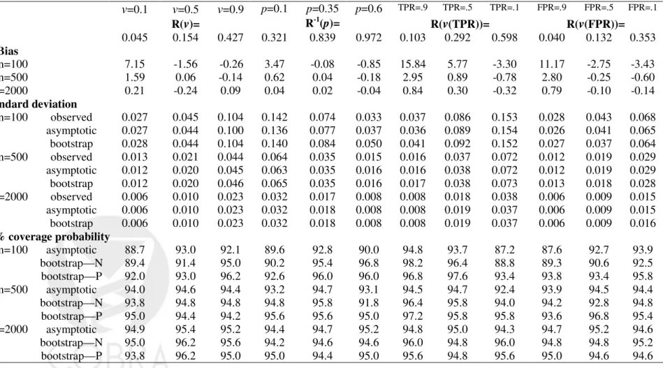
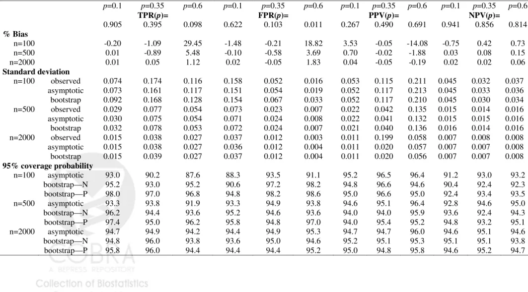
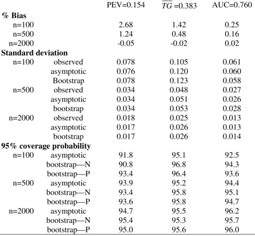
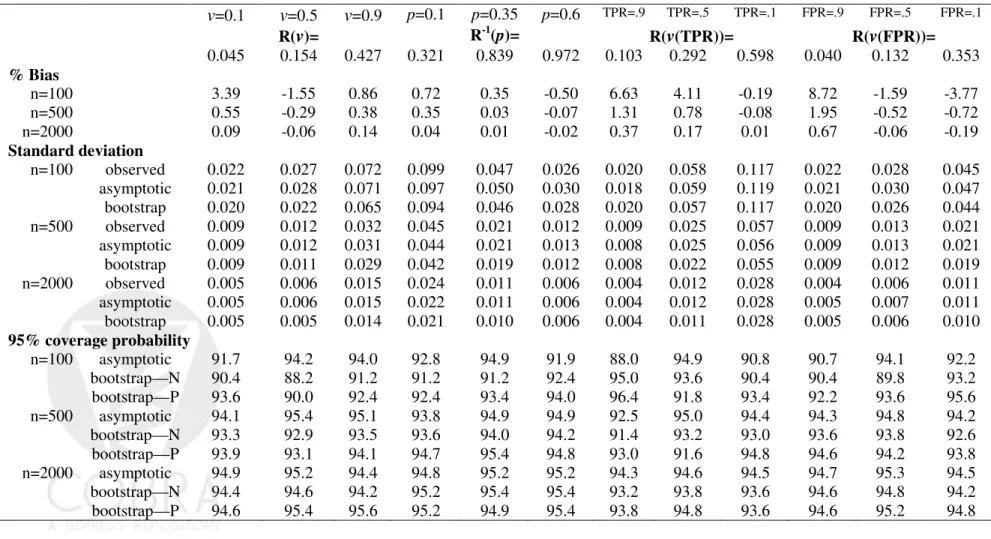
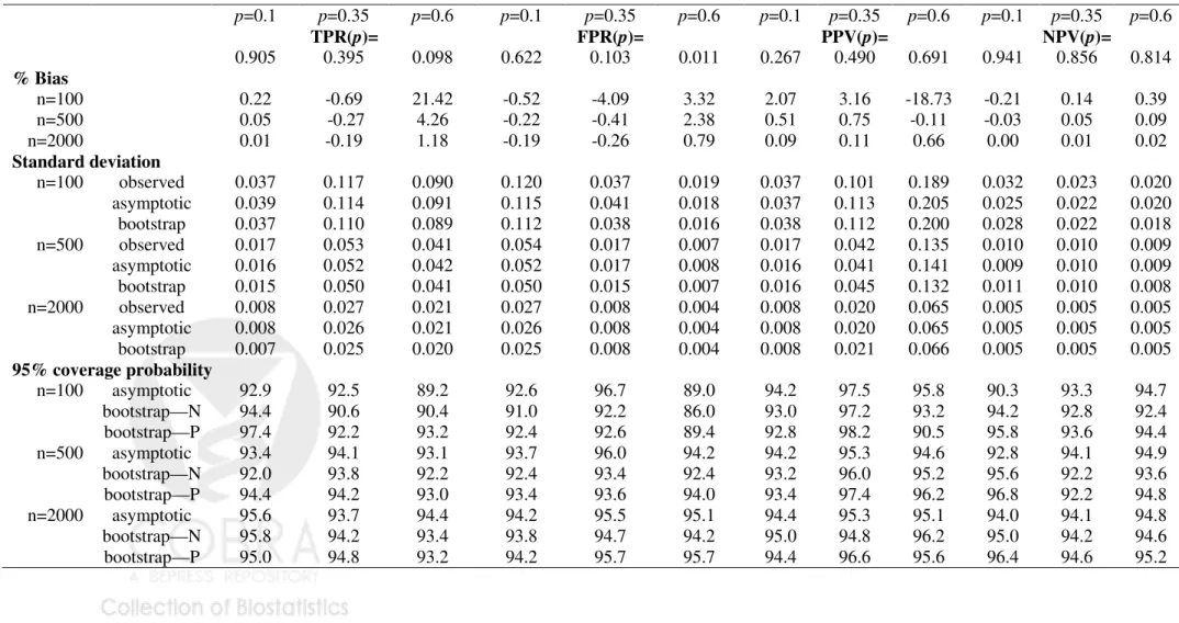
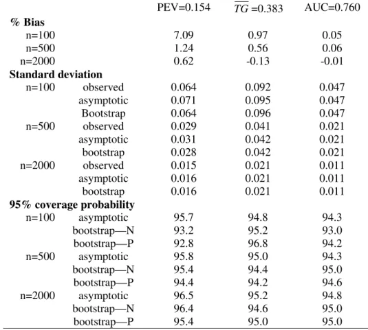
Table 1-3 displayed results for the summary indices under cohort study designs, while Table 4-6 are corresponding results under case-control study designs. Indeed, extensive simulation results for estimates of points on the predictiveness curve,R(ν) andR−1(p), were
already reported by Huang and Pepe (2008a). For completeness, we also included results for these two estimates under our simulation. We found little bias in the estimated values. Moreover estimated standard deviations based on asymptotic theory agree well with the actual standard deviations and with those estimated from bootstrap resampling. Coverage probabilities were excellent when sample sizes were moderate to large. We observed some under-coverage and some over coverage with small sample sizes (n =nD +nD¯ = 100). Not
surprisingly this occurred primarily at the boundaries of the case and control distributions and was not an issue for the overall summary measures, PEV, TG and AUC. Generally, coverage based on percentiles of the bootstrap distribution are somewhat better than those based on assumptions of normality, but the difference shrinks for larger n.
7
The Cystic Fibrosis Data
Cystic fibrosis is an inherited chronic disease that affects the lungs and digestive system of people. A defective gene and its protein product cause the body to produce unusually thick, sticky mucus which clogs the lungs and leads to life-threatening lung infections, and also obstructs the pancreas and stops natural enzymes from helping the body break down and absorb food. The main culminating event that leads to death is acute pulmonary exacerbations, i.e. lung infection requiring intravenous antibiotics.
The data for analysis here is from the Cystic Fibrosis Registry, a database maintained by the Cystic Fibrosis Foundation that contains annually updated information on over 20,000 people diagnosed with CF and living in the USA. In order to illustrate our methodology, we consider FEV1, a measure of lung function, and weight, a measure of nutritional status,
as measured in 1995 to predict occurrence of pulmonary exacerbation in 1996. Data from 12,802 patients 6 years of age and older are analyzed. 5245 subjects (41%) had at least one pulmonary exacerbation. A child’s weight is standardized for age and gender by reporting his/her percentile value in a healthy population of children of the same age and gender (Hamill,et al., 1977), while FEV1 is standardized for age, gender and height in a different
way, explicit formulae were provided by Knudson et al. (1983). We modelled the risk
functions using logistic regression models with weight and FEV1 entered the model as linear
terms, and both are negated to satisfy the assumption that increasing values are associated with increasing risk. Figure 1 shows the predictiveness curves for the entire cohort and Figure
2 shows the risk distributions separately for cases (those who had a pulmonary exacerbation) and for controls.
First, we use the entire cohort to estimate predictiveness summary measures for weight and lung function. Table 3 shows the point estimates discussed earlier in sections 2 and 3. Here we provide confidence intervals based on asymptotic distribution theory and on bootstrap resampling. Observe that standard deviations are all small and that corresponding confidence intervals are very tight. Bootstrap confidence intervals are almost identical to those based on asymptotic theory.
We used the summary indices as the basis for hypothesis tests to formally compare the predictive capacities of FEV1 and weight. The difference between estimates of the indices
was calculated and standardized using a bootstrap estimate of the variance of the differ-ence. By comparing these test statistics with quantiles of the standard normal distribution,
p-values were calculated. We see that differences between lung function and weight as
pre-dictive markers are statistically significant, no matter what summary index is employed. Note however that each test relates to a different question about predictive performance, depending on the particular summary index on which it is based. Asking if PEVs for weight and lung function are equal is not the same as asking if the proportion of subjects whose risks are less than 0.25, R−1(0.25), are equal. Asking if PEVs for weight and lung function
are equal is not the same as asking if the AUCs for risks associated with weight and FEV1
Next, we randomly sampled 1280 cases and 1280 controls from the entire cohort to form a nested case-control study sample that is about 1/5 th the size of the cohort. Table 4 presents results that use data on FEV1 and weight from the case-control subset and the estimate of
the overall incidence of pulmonary exacerbation from the entire cohort, ˆρ= 0.41. Estimates
of summary indices are very close to the cohort estimates but corresponding confidence intervals are much wider. Nevertheless conclusions remain the same. This demonstrates that in a study where predictive markers are costly to obtain, the nested case-control design could yield considerable cost savings.
Predictiveness summary measures, such as R(ν) andR−1(p), are based on a single point
on the predictiveness curve. Others, such as true and false positive rates and event rates, accumulate differences over part of the curve. Measures such as PEV, TG and AUC accumu-late differences over the entire curve. One might conjecture that measures that accumuaccumu-late differences would often be more powerful for testing if the predictiveness curves are equal. To investigate, we varied the case-control sample size and evaluatedp-values associated with
differences between the various summary measures. From Table 4, with a reasonably large case-control sample size (n=2560), we concluded that differences between almost all
sum-mary indices for the two markers are significantly different. However we see from Table 5 that as the size of the case-control study varies from medium (n=500) to small (n=100), the
point estimates of measures based on specific thresholds become much more variable and
p-values for differences between lung function and weight become statistically insignificant
marker remained firm when PEV, TG or AUC were used as the basis of hypothesis tests about equality of curves, even with very small sample sizes (n=100).
8
Concluding Remarks
This paper presents some new clinically relevant measures that quantify the predictive per-formance of a risk marker. New measures formally defined include TPR(p), FPR(p), PPV(p),
NPV(p),R(νT),R(νF), although several of these are already used informally in the applied
literature. We have previously argued for use ofR(ν) andR−1(p) in practice. In addition we
have provided new intuitive interpretations for some existing predictive measures, including the popular proportion of explained variation, PEV which is called the IDI by Pencina et
al. (2008), the standardized total gain, TG, and recently proposed risk reclassification
mea-sures, namely the NRI and the risk reclassification percent. We demonstrated that all of these measures are functions of the risk distribution, also known as the predictiveness curve. A fundamental initial step in the assessment of any risk model is to evaluate if risks calcu-lated according to the model reflect the probabilitiesP(D= 1|Y). The predictiveness curve can also be useful in making this assessment (Pepe et al., 2008) and is complemented by
use of the Hosmer-Lemeshow statistic (Hosmer and Lemeshow, 1989). In our cystic fibrosis example, the two linear logistic risk models, one for lung function and one for weight, both yield Hosmer-Lemeshow testp-values>0.05, indicating that they fit the observed data well.
the summary indices. Such has not been available for most of the measures heretofore, including the popular PEV measure. Our methods can now be used to construct confidence intervals for the summary indices. Simulation studies indicate that the methods are valid for application in practice with finite samples.
We also demonstrated in an example how summary indices can be used to make formal rigorous comparisons between markers. Such has only been possible previously for compar-isons based on the AUC or on point estimates of the predictiveness curve,R(ν) and R−1(p)
(Huang et al., 2007; Huang and Pepe, 2008).
Our methods accommodate cohort or case-control study designs. The latter are par-ticularly important in the early phases of biomarker development when biomarker assays are expensive or procurement of biological samples is difficult (Pepe et al., 2001). In such
settings nested case-control studies are much more feasible (Baker et al., 2002; Pepe et al.,
2008d). Our methodology is currently restricted to risk models that include a single marker or a predefined combination of markers. In practice studies often involve development of a marker combination and assessment of its performance. Compelling arguments have been provided in the literature for splitting a dataset into training and test subsets (Simon, 2006; Ransohoff, 2004). In these circumstances our methods apply to evaluation with the test data of the combination developed with the training data. It would be worthwhile however to explore use of cross validation techniques for simultaneous development and assessment of risk models using the summary indices we have described.
Which summary index should be recommended for use in practice? In our opinion, a summary index should not replace the display of the risk distributions (Figures 1 and 2) but should serve only to complement them. The choice of summary indices to report should be driven by the scientific objectives of the study. For example, if the objective is to risk stratify the population according to some risk threshold, below which treatment is not indicated and above which treatment is indicated, the corresponding proportions of the population that fall into the two risk strata, R−1(p
L) and 1−R−1(pL) would be key performance measures to report. Yet additional measures would also be of interest in this setting and should be reported including TPR(pL), FPR(pL), PPV(pL) and NPV(pL). When no risk thresholds
have been defined as clinically relevant, PEV or TG or AUC could complement the displays of risk distributions and serve as the basis of test statistics to test for the equality of differences between case and control risk distribution curves.
The final stages of evaluating a model for use in practice should incorporate notions of costs and benefits (i.e. utilities) that may be associated with decisions based on risk(Y).
However, specifying costs and benefits is typically very difficult in practice. Vickers and Elkin (2006) have recently proposed a standardized measure of expected utility for a prediction model that does not require explicit specifications of costs and benefits. The net benefit at risk thresholdpis defined asNB(p) =ρT P R(p)+(1−ρ)F P R(p)p/(1−p), and their decision curve plots NB(p) versus p. This weighted average of true and false positive rates could
complement descriptive plots of risk distributions. Moreover, the methods for inference that we have presented here give rise to methods for inference about decision curves too.
References
Baker, S.G., Kramer, B.S. and Srivastava, S. (2002) Markers for early detection of cancer: statistical guidelines for nested case-control studies. BMC Med. Res. Methodol.,2, 4.
Bura, E. and Gastwirth, J. L. (2001) The binary regression quantile plot: assessing the importance of predictors in binary regression visually. Biometrical J., 43, 5-21.
Cook, N.R. (2007) Use and misuse of the receiver operating characteristic curve in risk prediction. Circulation, 115, 928-935.
Cook, N.R., Buring, J.E. and Ridker, P.M. (2006) The effect of including c-reactive protein in cardiovascular risk prediction models for women. Ann. Intern. Med., 145, 21-29.
Expert Panel on Detection EaToHBCiA. (2001) Executive summary of the third report of the National Cholesterol Education Program (NCEP) Expert Panel on detection, evaluation, and treatment of high blood cholesterol in adults (Adult Treatment Panel III).J. Am. Med. Assoc., 285(19), 2486-2497.
Gail, M.H. and Pfeiffer, R.M. (2005) On criteria for evaluating models of absolute risk. Biostatistics, 6(2), 227-239.
Green, D.M. and Swets, J.A. (1996) Signal detection theory and psychophysics. New York:
Wiley.
Gu, W. and Pepe, M.S. (2009) Estimating the capacity for improvement in risk prediction with a marker. Biostatistics, 10(1), 172-186.
Gu, W. and Pepe, M.S. (2009a) Measures to summarize and compare the predictive capacity of markers. UW Biostatistics Working Paper Series.
Hamill, P.V., Drizd, T.A., Johnson, C.L., Reed, R.B. and Roche, A.F. (1977) NCHS growth curves for children birth-8 years. United States, Vital Health Statistics 11, pp. 1-74. Washington, DC.
Hosmer, D.W. and Lemeshow, S. (1989) Applied Logistic Regression (section 5.2.2). New
York: Wiley.
Hu, B., Palta, M. and Shao, J. (2006) Properties of R2 statistics for logistic regression.
Statist. Med.,25(8), 1383-1395.
Huang, Y. and Pepe, M.S. (2008a) Semiparametric and nonparametric methods for
evaluat-ing risk prediction markers in case-control studies. Biometrika (in press).
Huang, Y. and Pepe, M.S. (2008b) A parametric ROC model based approach for evaluat-ing the predictiveness of continuous markers in case-control studies. Biometrics, doi:
10.1111/j.1541-0420.2005.00454.x
Huang, Y., Pepe, M.S. and Feng, Z. (2007) Evaluating the predictiveness of a continuous marker. Biometrics, 63(4), 1181-1188.
Hunink, M., Glasziou, P., Siegel, J., Weeks, J., Pliskin, J., Elstein, A. and Weinstein, M. (2006) Decision making in health and medicine. Cambridge University Press.
Janes, H., Pepe, M.S. and Gu, W. (2008) Assessing the value of risk predictions using risk stratification tables. Ann. Intern. Med.,149(10), 751-760.
Janssens, A.C.J.W., Aulchenko, Y.S., Elefante, S., Borsboom, G.J.J.M, Steyerberg, E.W. and van Duijn, C.M. (2006) Predictive testing for complex diseases using multiple genes: Fact or fiction? Genet. Med.,8(7), 395-400.
Knudson, R.J., Lebowitz, M.D., Holberg, C.J. and Burrows, B. (1983) Changes in the normal maximal expiratory flow-volume curve with growth and aging. Am. Rev. Respir. Dis.,
127, 725-734.
Pencina, M.J., D’Agostino Sr., R.B., D’Agostino Jr., R.B. and Vasan, R.S. (2008) Evaluating the added predictive ability of a new marker: From area under the ROC curve to reclassification and beyond. Statist. Med.,27, 157-172.
Pepe, M.S. (2003) The Statistical Evaluation of Medical Tests for Classification and
Predic-tion. Oxford University Press.
Pepe, M.S., Etzioni, R., Feng, Z., Potter, J.D., Thompson, M.L., Thornquist, M., Winget, M. and Yasui, Y. (2001) Phases of biomarker development for early detection of cancer. J. Natl. Cancer Inst., 93, 10541061.
Pepe, M.S., Feng, Z. and Gu, W. (2008b) Comments on ’Evaluating the added predictive ability of a new marker: From area under under the ROC curve to reclassification and beyond’. Statist. Med., 27, 173-181.
Pepe, M.S., Feng, Z., Huang, Y., Longton, G.M., Prentice, R., Thompson, I.M. and Zheng, Y. (2008a) Integrating the predictiveness of a marker with its performance as a classifier. Am. J. Epidemiol., 167(3), 362-368.
Pepe, M.S. and Janes, H. (2008c) Gauging the performance of SNPs, biomarkers and clinical factors for predicting risk of breast cancer. J. Natl. Cancer Inst., 100(14), 978-979.
Pepe, M.S., Feng Z, Janes H, Bossuyt P and Potter J. (2008d) Pivotal evaluation of the accuracy of a biomarker used for classification or prediction: Standards for study design Journal of the National Cancer Institute, 100(20), 1432-1438
Pepe, M.S., Janes, H. and Gu, W. (2007) Letter by Pepe et al regarding the article, “Use and Misuse of the Receiver Operating Characteristic Curve in Risk Prediction”.
Cir-culation, 116, e132.
Prentice, R.L. and Pyke, R. (1979) Logistic disease incidence models and case-control studies. Biometrika,66(3), 403-411.
Qin, J. (1998) Inferences for case-control and semiparametric two-sample density ratio mod-els. Biometrika, 85(3), 619-630.
Qin, J. and Lawless, J. (1994) Empirical likelihood and general estimating equations. Ann.
Statist., 66(3), 403-411.
Qin, J. and Zhang, J. (1997) Empirical likelihood and general estimating equations. Ann.
Statist., 22(1), 300-325.
Qin, J. and Zhang, J. (2003) Using logistic regression procedures for estimating receiver operating characteristic curves. Biometrika, 84(3), 609-618.
Ransohoff, D.F. (2004) Rules of evidence for cancer molecular-marker discovery and valida-tion. Nat. Rev. Cancer,4(4), 309-314.
Ridker, P.M., Hennekens, C.H., Buring, J.E. and Rifai, N. (2000). C-reactive protein and other markers of inflammation in the prediction of cardiovascular disease in women. N. Engl. Med.,342, 836-843.
Ridker, P.M., Paynter, N.P., Rifai, N., Gaziano, J.M. and Cook, N.R. (2008) C-reactive protein and parental history improve global cardiovascular risk prediction: The risk score for men. Circulation, 118, 2243-2251.
Simon, R. (2006) Roadmap for developing and validating therapeutically relevant genomic classifiers. J. Clin. Oncol., 23(29), 7332-7341.
Stern, R.H. (2008) Evaluating new cardiovascular risk factors for risk stratification. J. Clin.
Hypertens., 10(6), 485-488.
Vickers, A.J. and Elkin, E.B. (2006) Decision curve analysis: a novel method for evaluating prediction models. Med. Decis. Making, 26(6), 565-574.
Ware, J.H. and Cai T. (2008) Comments on ‘Evaluating the added predictive ability of a new marker: From area under the ROC curve to reclassification and beyond’. Statist.
Med., 27, 185-187.
Youden, W.J. (1950) Index for rating diagnostic tests. Cancer, 3, 3235.
Zheng, B and Agresti, A. (2000) Summarizing the predictive power of a generalized linear model. Stat Med., 19(13), 1771-1781.
Appendix: Asymptotic Theory
To simplify notation, we suppose the risk model is logistic linear in Y:
logit{G(θ, Y)}=θ0+θ1Y.
I. Cohort Design
In a cohort study the log likelihood function is
l(θ|Y1, ..., Yn) = nD X i=1 log exp(θ0+θ1Yi) 1 +exp(θ0+θ1Yi) + nD¯ X i=1 log 1 1 +exp(θ0+θ1Yi) . (15)
Let ˆθ0, ˆθ1be the maximum likelihood estimators (MLE) ofθ0,θ1based on (15). The following
results are well known.
Result 1 Let A0(θ, t) = Z t −∞ exp(θ0+θ1y) (1 +exp(θ0+θ1y))2 dF(y) A1(θ, t) = Z t −∞ yexp(θ0+θ1y) (1 +exp(θ0+θ1y))2 dF(y) A2(θ, t) = Z t −∞ y2exp(θ 0+θ1y) (1 +exp(θ0+θ1y))2 dF(y) A(θ, t) = A0(θ, t) A1(θ, t)T A1(θ, t) A2(θ, t) ,
and A(θ) =A(θ,∞). If A(θ)−1 exists, √ n ˆ θ0−θ0 ˆ θ1−θ1 → dN(0, A(θ)−1).
We can also write √n(ˆθ −θ) = √1
n Pn i=1`θ(Yi) +op(1), where `θ(Yi) = A(θ)−1l˙θ(Yi), i = 1, ..., n. And ˙ lθ(Yi) = ∂l(θ|Yi)/∂θ0 ∂l(θ|Yi)/∂θ1 = Di−exp(θ0+θ1Yi)/(1 +exp(θ0+θ1Yi)) DiYi−Yiexp(θ0+θ1Yi)/(1 +exp(θ0+θ1Yi)) . Result 2 Asn → ∞, √ n(ˆρ−ρ)→dN(0, ρ(1−ρ)), √ n( ˆF(t)−F(t))→dN(0, F(t)(1−F(t))), √ n( ˆFD(t)−FD(t))→dN(0, FD(t)(1−FD(t))/η), √n( ˆF ¯ D(t)−FD¯(t))→dN(0, FD¯(t)(1−FD¯(t))/(1−η)), where η≡nD/n.
Lemma 1Let BD,0(t) = Z t −∞ 1 1 +exp(θ0+θ1y) dFD(y) BD,1(t) = Z t −∞ y 1 +exp(θ0+θ1y) dFD(y) BD,¯ 0(t) = Z t −∞ exp(θ0+θ1y) 1 +exp(θ0+θ1y) dFD¯(y) BD,¯ 1(t) = Z t −∞ yexp(θ0+θ1y) 1 +exp(θ0+θ1y) dFD¯(y),
and useBD,0, BD,1, BD,¯0 and BD,¯ 1 for the limits at t=∞.
Then we have cov(√n(ˆθ−θ),√n( ˆF(t)−F(t)) =A(θ)−1 ρBD,0(t)−(1−ρ)BD,¯0(t) ρBD,1(t)−(1−ρ)BD,¯1(t) cov(√n(ˆθ−θ),√n( ˆFD(t)−FD(t)) =A(θ)−1 BD,0(t)−FD(t)BD,0 BD,1(t)−FD(t)BD,1
cov(√n(ˆθ−θ),√n( ˆFD¯(t)−FD¯(t)) =A(θ)−1 −BD,¯0(t) +FD¯(t)BD,¯ 0 −BD,¯1(t) +FD¯(t)BD,¯ 1 Proof:
We prove the first result and proofs of the other two results follow from similar arguments.
cov(√n(ˆθ−θ),√n( ˆF(t)−F(t)) =cov(√1 n n X i=1 A(θ)−1l˙θ(Yi), 1 √ n n X i=1 (I(Yi ≤t)−F(t))) =cov(A(θ)−1l˙ θ(Y), I(Y ≤t)−F(t))) =A(θ)−1E( ˙lθ(Y)×I(Y ≤t)) =A(θ)−1{ρE( ˙lθ(YD)×I(YD ≤t)) + (1−ρ)E( ˙lθ(YD¯)×I(YD¯ ≤t))} =A(θ)−1 ρBD,0(t)−(1−ρ)BD,¯ 0(t) ρBD,1(t)−(1−ρ)BD,¯ 1(t)
Proof of Theorem items (i), (ii) and (iii) We show the proof for item (i). The proofs for items (ii) and (iii) follow similar arguments.
√
n( ˆR−1(p)−R−1(p)) = √n( ˆF(G−1(ˆθ, p))−F(G−1(θ, p)))
where
Rn =√n( ˆF(G−1(ˆθ, p))−Fˆ(G−1(θ, p)))−√n(F(G−1(ˆθ, p))−F(G−1(θ, p))) =op(1)
by equicontinuity of the process √n( ˆF −F). Earlier results and the delta method then imply: σ1(p)2 =var(√n( ˆR−1(p)−R−1(p))) =var(√n( ˆF(G−1(θ, p))−F(G−1(θ, p)))) +var(√n(F(G−1(ˆθ, p))−F(G−1(θ, p)))) + 2cov√n( ˆF(G−1(θ, p))−F(G−1(θ, p))),√n(F(G−1(ˆθ, p))−F(G−1(θ, p)))) (16) =R−1(p)(1−R−1(p)) + (∂R− 1(p) ∂θ ) T A(θ)−1(∂R− 1(p) ∂θ ) + 2(∂R− 1(p) ∂θ ) T A(θ)−1 ρBD,0(G−1(θ, p))−(1−ρ)BD,¯ 0(G−1(θ, p)) ρBD,1(G−1(θ, p))−(1−ρ)BD,¯ 1(G−1(θ, p)) .
The last equality follows from Result 2 (for variance of ˆF), Result 1 (for variance of ˆθ) and
Lemma 1 (for covariance of ( ˆF ,θˆ)).
Proof of Theorem items (iv) and (v) We write ˆ P P V(p) = ρˆ 1−ρˆ ˆ T P R(p) ˆ F P R(p),