Documents de Travail du
Centre d’Economie de la Sorbonne
Scale-dependence of the Negative Binomial Pseudo-Maximum Likelihood Estimator
Clément BOSQUET, Hervé BOULHOL
2010.92
Scale-dependence of the Negative Binomial
Pseudo-Maximum Likelihood Estimator
∗
Clément Bosquet
†Hervé Boulhol
‡November 9, 2010
Abstract
Following Santos Silva and Tenreyro (2006), various studies have used the Poisson Pseudo-Maximum Likelihood to estimate gravity specications of trade ows and non-count data models more generally. Some papers also report results based on the Negative Binomial estimator, which is more general and encompasses the Poisson assumption as a special case. This note shows that the Negative Binomial estimator is inappropriate when applied to a continuous dependent variable which unit choice is arbitrary, because estimates articially depend on that choice.
JEL Codes: C13, C21, F10
Keywords: pseudo-maximum likelihood methods, negative binomial estimator, Poisson regression, gamma PML
∗We are particulary grateful to Thierry Mayer who provided data as well as useful suggestions at an early
stage. We also would like to greatly thank Joao Santos Silva, Thierry Magnac, Pierre-Philippe Combes and Lionel Fontagné for useful comments, as well as participants of the GREQAM PhD Students lunch seminar, the 2009 RIEF doctoral meetings, the 2009 EEA congress, the 2009 AFSE congress and the 2009 ASSET congress.
†GREQAM, Université Aix-Marseille, corresponding author, [email protected] ‡OECD and Université Paris Panthéon-Sorbonne
Résumé
Depuis l'article de Santos Silva et Tenreyro (2006), plusieurs études ont utilisé le pseudo-maximum de vraisemblance (PMV) avec loi de Poisson pour estimer les équations de gravité des ux de commerce et, plus généralement, des modèles avec données continues (c'est-à-dire non discrètes). Certains papiers rapportent aussi des résultats obtenus à l'aide du PMV avec loi binomiale négative, estimateur plus général dont la loi de Poisson est un cas particulier. Cette note montre que l'estimateur du PMV avec loi binomiale négative est inapproprié lorsque la variable à expliquer est mesurée avec une unité dont le choix est arbitraire, parce que les estimations dépendent articiellement de ce choix.
Mots clés : méthodes du pseudo-maximum de vraisemblance, estimateur avec loi binomiale négative, régression de Poisson, pseudo-maximum de vraisemblance avec loi gamma
1 Introduction
Pseudo-Maximum Likelihood (PML) methods were introduced and then derived for Poisson models by Gourieroux, Monfort and Trognon (1984a,b). Following these seminal works, the Poisson PML (PPML) estimator, which assumes proportionality between the conditional variance and the conditional expectancy of the dependent variable, has often been used for count data models. However, beyond count data, Gourieroux et al. (1984b) note that "the pseudo-maximum likelihood method with Poisson family may be applied even if the dependent variable is any real number".
Santos Silva and Tenreyro (2006) highlight the advantages of this estimator for gravity equations of bilateral trade ows specied in levels, relative to the common practice of estimating these equations in log-levels by Ordinary Least Squares. Indeed, these authors show that the log-linear specication leads to biased estimates following Jensen's inequality, due to heteroskedasticity
in trade levels.1 Moreover, they provide some evidence that the PPML estimator is more
ecient than the nonlinear least squares estimator of the trade specication in level.
As a result, a number of empirical studies of trade ows apply the PPML estimator. As an extension, some researchers consider other PML estimators based on non-Poisson distributions such as gamma according to which the variance is proportional to the square of the conditional mean. The Negative Binomial (NB) PML estimator has also been increasingly used recently in trade as well as mergers and acquisitions studies, including Head, Mayer and Ries (2009), Burger, van Oort and Linders (2009), Briant, Combes and Lafourcade (2009), Westerlund and Wilhelmsson (2009) and Garita and van Marrewijk (2008). The NB distribution assumes that the conditional variance is a linear combination, to be estimated, of the conditional mean and of its square. The NB PML estimator is appealing because it encompasses both PPML and gamma PML as special cases.
This note shows that the NB PML estimator is inappropriate when applied to continuous dependent variables, such as trade or M&A ows, for which the choice of the unit measure is arbitrary. For example, in the case of trade equations, the NB PML estimated parameters
1Because E(Log x) 6= Log E(x) the expected value of the logarithm of trade ows depends on higher
moments, including the variance. Since the variance of the residuals is likely to depend on explanatory variables, estimators using the log specication are biased.
depend articially on whether trade ows are measured in thousands of dollars, in billions of dollars or in millions of euros. More precisely, when ows are measured in small units (e.g. thousands of dollars), the NB PML converges towards the gamma PML estimator. In contrast, when ows are measured in large units (e.g. trillions of dollars), the NB PML converges towards the Poisson PML estimator. This scale dependence has been unnoticed so far.
As an interesting case, Garita and van Marrewijk (2008) use the NB PML estimator with either the value or the number of mergers and acquisitions as the dependent variable. According to this note, the estimator based on the value will articially depend on the choice of unit, while in principle the estimator based on the number is immune to this problem. However, even for count data, the NB estimator is sensitive to whether the dependent variable is measure in the actual number, in hundreds, in thousands, etc.
Section 2 provides the proof of the scale-dependence of the NB estimator, and section 3 illustrates this proposition with an application based on the trade gravity equation.
2 Proof
The specication is yi = exp(Xi β +ui) where ui is the residual. The rst-order conditions
for PPML, NB PML and gamma PML are, respectively (Gourieroux, Monfort and Trognon ; 1984a,b): PPML: X i yi−exp(Xi β) Xi = 0 (1) NB PML: X i 1 +α exp(Xi β) −1 yi−exp(Xi β) Xi = 0 (2) gamma PML: X i exp(−Xi β) yi−exp(Xi β) Xi = 0 (3)
Whereas the underlying assumption of the PPML and gamma PML is that the conditional variance is proportional to the conditional expectancy and to its square, respectively, the
NB PML assumes that V ar(y|X) = E(y|X) +α E2(y|X), where α is a constant, generally
considered to be positive. Eq. (1-3) conrm that whenα→0, NB PML→PPML, while when
α→ ∞, NB PML → gamma PML.
This note focuses on the impact of using y˜ = λ y as the dependent variable instead of y
where λ is a scalar that can be either very small or very large depending on the unit choice.
The rst-order conditions indicate that both the Poisson and gamma estimator are independent
of scale, as only the constant, denoted β0, is aected by the linear transformation according
to β˜0(λ) = β0+Log λ, such that exp( ˜β0(λ)) = λ exp(β0). This implies that exp(Xi β˜(λ)) = λ exp(Xi β) ∀i, and the FOC (1) and (3) are unaected by scale2:
˜ β0(λ) = β0+Log λ ˜ βk(λ) = βk ∀k6= 0 ⇒ (4) PPML: X i ˜ yi−exp(Xi β˜) Xi = 0⇔λ X i yi−exp(Xi β) Xi = 0 (5) gamma PML: X i exp(−Xi β˜) y˜i−exp(Xi β˜) Xi = 0 ⇔ X i exp(−Xi β) yi−exp(Xi β) Xi = 0 (6)
In contrast, the rst-order condition for NB PML (eq. 2) is sensitive to λ. When y˜is the
dependent variable, that condition is:
X i 1 + ˜α exp(Xi β˜) −1 ˜ yi−exp(Xi β˜) Xi = 0 (7)
Forβ˜to be unaected (except the intercept) by the transformation, the FOC must be:
X i 1 + ˜α λ exp(Xi β) −1 λ yi−exp(Xi β) Xi = 0 (8)
The comparison of (2) and (8) implies that the condition under which the NB PML estimator
is independent of λ is α˜(λ) = α/λ, with α≡α˜(λ= 1).3
However, this condition is violated in general. Let us rst consider the two-step estimator implemented in various econometric softwares. The rst step consists in computing a consistent
2β≡β˜(λ= 1).
3Another way to see this is as follows. The NB PML assumption is V ar(˜y(λ)|X) = E[˜y(λ)|X] +
˜
α(λ)E2[˜y(λ)|X]. Under the condition thatβ˜is independent fromλ(exceptβ˜0), this becomes: λ2V ar[y|X] =
λ E[y|X] +λ2 α˜(λ) E2[y|X] ⇔V ar[y|X] = 1/λE[y|X] +λ α˜(λ)E2[y|X]. Independence of the estimator
with respect to λimplies thatλα˜(λ) =α.
estimator, e.g. PPML which is used in most softwares (Stata, SAS), andyˆidenotes the rst-step
estimated observations. In a second step,α is estimated by OLS from the following regression:
(yi −yˆi)2−yˆi =α yˆi2+i (9)
where i is a residual, which yields:
ˆ α= P i[(yi−yˆi)2−yˆi] ˆyi2 P iyˆi4 (10) This corresponds to the Quasi-generalized PML estimator for NB proposed by Gourieroux et al. (1984b), renamed "two-step NB" by Wooldridge (1999), and for which Head et al. (2009) provide a Stata code.
What happens to this estimator when the linear transformation y˜ = λ y is used as the
dependent variable? As shown before, the rst-step PPML estimator is unaected by scale,
hence yˆ˜i(λ) =λ yˆi. It follows that:
λ αˆ˜(λ) = λ P i[( ˜yi−yˆ˜i) 2−yˆ˜ i] ˆy˜i2 P iyˆ˜ 4 i =λ P i[λ 2 (y i−yˆi)2−λ yˆi] λ2 yˆi2 λ4 P iyˆi4 (11) = P i[λ (yi−yˆi)2−yˆi] ˆyi2 P iyiˆ 4 = ˆα+ (λ−1) P i(yi−yˆi)2 yˆi2 P iyiˆ 4
which proves that:
• λ αˆ˜(λ)6= ˆα as soon as λ6= 1 ;
• when λ→+∞,λ α˜ˆ(λ)→+∞ and NB PML→ gamma PML ;
• when λ → 0, λ αˆ˜(λ) → αˆ− Pi(yi−yˆi) ˆyi2 P iyˆi4 = − P iyˆi3 P
iyˆi4. When the software constrains the
estimated value to be positive (e.g. Stata), λ αˆ˜(λ)→0, and NB PML → PPML.
Section 3 provides an empirical example illustrating these results.
This problem is not an artefact of using a two-step estimator. Even the theoretical NB PML estimator exhibits scale dependence. To see this, calculate instead of eq. (9) the FOC on
α. The full log-likelihood is:4 LogL = X i Log Γ(α −1+y) Γ(α−1)Γ(y+ 1) −α−1Log[α] +yi Xi β (12) − α−1+yi
Log[1 +α exp(Xi β)]−Log[α]
where Γ is the standard Gamma function.5
While dierentiating this expression with respect to β leads to (2), dierentiating with
respect to α entails:6 α−2X i Log[1 +α exp(Xi β)] + yi−exp(Xi β) α−1+exp(Xi β) − +∞ X k=0 yi (k+α−1)(k+α−1+yi) ! = 0 (13)
With the linear transformation, the FOC becomes:
˜ α−2X i Log[1 + ˜α exp(Xi β˜)] + ˜ yi−exp(Xi β˜) ˜ α−1+exp(X i β˜) − +∞ X k=0 ˜ yi (k+ ˜α−1)(k+ ˜α−1+ ˜y i) ! = 0 (14)
As seen above, the non-scale-dependence ofβ(except the intercept) is equivalent toexp(Xiβ˜(λ)) =
λ exp(Xi β) ∀iand α˜(λ) =α/λ. By absurd reasoning, the FOC is then written:
λ2α−2X i Log[1 +α exp(Xi β)] + λ yi−λ exp(Xi β) λ α−1+λ exp(X i β) − +∞ X k=0 λ yi (k+λ α−1)(k+λ α−1+λ y i) ! = 0 (15) ⇔X i Log[1 +α exp(Xi β)] + yi−exp(Xi β) α−1+exp(X i β) ! =X i +∞ X k=0 yi (kλ +α−1)(k λ +α −1+y i) (16)
which is absurd given thatα is dened according to (13) by:
⇔X i Log[1 +α exp(Xi β)] + yi−exp(Xi β) α−1+exp(X i β) ! =X i +∞ X k=0 yi (k+α−1)(k+α−1+y i) (17)
That is, the FOC on α is scale-dependent as the right hand side termP
i +∞ P k=0 yi (k λ+α−1)( k λ+α−1+yi)
in eq. (16) depends onλ. The empirical example developed in the following section illustrates
4Calculations details are provided in Appendix A. 5Γ(x) =R+∞
0 t
x−1 e−tdt.
6Calculations details are provided in Appendix B.
that the direct estimation of α˜(λ) based on eq. (14) violates the condition that λ α˜(λ) is
independent of scale.
3 Application to the trade gravity equation
3.1 Data
Trade ow data are taken from the IMF Direction Of Trade Statistics (DOTS) database. For
the year 2000, there are 21,543 non-zero ows between 196 trading partners.7 The geographical
variables (distance between countries, common border, common language and colonial linkage
dummies) are provided by the CEPII database8, and the FTA data are based on Fontagné and
Zignago (2007) who improve those used by Baier and Bergstrand (2007).
3.2 Specication
The bilateral trade equation is estimated following Anderson and van Wincoop (2003) according to:
xij =exp(β0+β1 Log dij +β2 Bij +β3 Lij +β4 Cij +β5 F T Aij +F Xi+F Mj)uij (18)
where xij is the value of export from country i to country j, F Xi and F Mj are exporting
and importing countries xed eects, respectively. Bij,Lij and Cij are the traditionnal control
covariates: common border, common ocial language and colonial linkage dummies, respectively.
The uij are the multiplicative error terms of the nonlinear estimates. Following Anderson and
van Wincoop (2003), importer and exporter xed eects are used to control for multilateral resistance terms as well as for the income levels of both importers and exporters.
7Focusing on non-zero ows is sucient for illustration purposes. Including zero ows or focusing on other
years unsurprisingly leads to the same conclusion as the proof in section 2 is general.
8http://www.cepii.fr/anglaisgraph/bdd/distances.htm, Centre d'Etudes Prospectives et d'Informations
Internationales.
3.3 Results
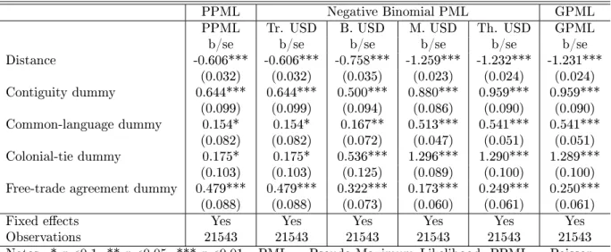
Table 1 shows the estimates of equation (18) from the PPML and gamma PML estimators, in the rst and last columns, respectively. The columns in between report the NB PML estimates based on dierent unit values for trade ows. Is is computed either by the Stata nbreg (or glm with nbinomial family) estimator, the SAS proc genmod procedure or the two-step Head et al. (2009)'s code, which yield identical estimated values. When ows are measured with a very large unit (trillions of US$), which means that ow values are very small, NB PML and PPML estimates are visually identical. At the other extreme, when ows take very large values (i.e. when the unit is small such as thousands of US$), the NB PML are very close to the gamma PML estimates. This illustrates that the NB PML estimator is inappropriate as the estimates depend arbitrarily on the unit choice of the dependent variable.
Table 2 compares the dispersion parameter α˜(λ) estimated by various NB PML estimators,
and shows that for all of them the condition under which these estimators are not sensitive
to scale (i.e. λ α˜(λ) does not depend on λ) is violated. The NB PML estimators that are
compared are: that computed by Stata, that by SAS, the two-step estimator using PPML in the rst step according to eq. (9-11), the two-step estimator using the geometric estimator in
the rst step according to Head et al. (2009), and the one-step estimator computing α˜ such
that likelihood is maximized (eq. 14, using Newton algorithm and PPML for β). Both Stata
and SAS compute an iterated estimator, reestimating eq. (9-11) at each step and starting
with PPML, with α˜ being the nal iterated value, and yield similar results. For all these NB
PML estimators, λα˜ depend onλ, converging towards zero whenλ becomes small and innity
when λ becomes large. That is, all NB PML estimators converge towards PPML and GPML,
respectively.
4 Conclusion
Although it is being increasingly used, the NB PML is not appropriate when the unit choice of the dependent variable is arbitrary.
Appendix
A Log-likelihood of the Negative Binomial estimator
Negative Binomial density:
P r[Y =y] = Γ(α −1+y) Γ(α−1)Γ(y+ 1) α−1 α−1+µ !α−1 µ µ+α−1 !y (19) Log-likelihood: LogL=X i Ai+α−1 Log[α−1]−Log[α−1+µi] +yi Log[µi]−Log[µi+α−1] (20) with: Ai =Log Γ(α−1+y i) Γ(α−1)Γ(y i+ 1) ! (21)
Replacing µi byexp(Xi β)leads to:
LogL=X
i
Ai−α−1
Log[α] +Log[α−1+exp(Xi β)]
+yi
Log[exp(Xi β)]−Log[exp(Xi β) +α−1]
(22)
⇔LogL=X i
Ai−α−1Log[α]−α−1Log[α−1+exp(Xi β)] +yi Xi β−yi Log[exp(Xi β) +α−1]
(23) ⇔LogL =X i Ai−α−1Log[α] +yi Xi β− α−1+yi Log[α−1+exp(Xi β)] (24) Rewriting:
Log[α−1+exp(Xi β)] =Log[α−1 1 +α exp(Xi β)
] =Log[α−1] +Log[1 +α exp(Xi β)] (25)
yields:
LogL=X
i
Ai−α−1Log[α] +yi Xi β− α−1+yi
Log[1 +α exp(Xi β)]−Log[α]
(26)
Rewriting: Bi =yi Xi β− α−1+yi Log[1 +α exp(Xi β)] (27) leads to: LogL =X i Ai+Bi−α−1Log[α] + α−1+yi Log[α] =X i Ai+Bi+yi Log[α] (28) Consistent with P
iBi as the objective function with respect to β in Gourieroux, Monfort and
Trognon (1984a).
B First-order condition with respect to
α
For derivating the Gamma function, the digamma function, denotedψ is used:9
ψ(x) =D Log[Γ(x)] = Γ 0(x) Γ(x) =−γ− 1 x +x +∞ X k=1 1 k(k+x) (29)
where D is the dierential operator andγ the Euler-Mascheroni' constant.
Dropping terms without α from (28) leads to the objective function with respect to α:
X i Log Γ(α −1 +y i) Γ(α−1) ! − α−1+yi
Log[1 +α exp(Xi β)] +yi Log[α] (30)
Rewriting: Ci =Log Γ(α −1+y i) Γ(α−1) ! (31) and: Di =− α−1+yi
Log[1 +α exp(Xi β)] +yi Log[α] (32)
the FOC would be P
iC 0 i +D
0
i = 0. Dierentiating Ci leads to:
Ci0 =−α−2 −γ− 1 α−1+y i +(α−1+yi) +∞ X k=1 1 k(k+α−1+y i) − −γ− 1 α−1+α −1 +∞ X k=1 1 k(k+α−1) ! (33)
9Andrews, Askey and Roy (1999)
Ci0 =−α−2 1 α−1 − 1 α−1+yi + (α −1+y i) +∞ X k=1 1 k(k+α−1+yi) −α −1 +∞ X k=1 1 k(k+α−1) ! (34) Ci0 =−α−2 yi α−1(α−1+yi)+yi +∞ X k=1 1 k(k+α−1+yi)+α −1 +∞ X k=1 1 k(k+α−1+yi)− 1 k(k+α−1) ! (35)
Rewriting Ei, the last term within the parenthesis:
Ei =α−1 +∞ X k=1 1 k(k+α−1+y i) − 1 k(k+α−1) =α−1 +∞ X k=1 −yi k(k+α−1+y i)(k+α−1) (36) =−yi +∞ X k=1 α−1 k(k+α−1+y i)(k+α−1) (37) leads to: Ci0 =−α−2 yi α−1(α−1 +y i) +yi +∞ X k=1 1 k(k+α−1+y i) −yi +∞ X k=1 α−1 k(k+α−1+y i)(k+α−1) ! (38) ⇔Ci0 =−α−2 yi α−1(α−1+y i) +yi +∞ X k=1 1 (k+α−1)(k+α−1+y i) ! (39) ⇔Ci0 =−α−2 +∞ X k=0 yi (k+α−1)(k+α−1+y i) (40)
Dierentiating Di leads to:
Di0 =α−2 Log[1 +α exp(Xi β)]− α−1+yi exp(Xi β) 1 +α exp(Xi β) + yi α (41) ⇔Di0 =α−2 Log[1 +α exp(Xi β)] + yi−exp(Xi β) α 1 +α exp(Xi β) (42) ⇔Di0 =α−2 Log[1 +α exp(Xi β)] + yi−exp(Xi β) α−1+exp(Xi β) ! (43)
which yields the FOC with respect to α:
α−2X i Log[1 +α exp(Xi β)] + yi−exp(Xi β) α−1+exp(X i β) − +∞ X k=0 yi (k+α−1)(k+α−1+y i) ! = 0 (44)
References
Anderson, J. and van Wincoop, E. (2003), `Gravity with Gravitas: A Solution to the Border Puzzle', American Economic Review 93(1), 170192.
Andrews, G., Askey, R. and Roy, R. (1999), Special Functions, Cambridge: Cambridge University Press.
Baier, S. L. and Bergstrand, J. H. (2007), `Do Free Trade Agreements Actually Increase Members International Trade?', Journal of International Economics 71(1), 7295.
Briant, A., Combes, P.-P. and Lafourcade, M. (2009), `Product Complexity, Quality of Institutions and the Pro-Trade Eect of Immigrants', CEPR Discussion Paper (7192). Burger, M., van Oort, F. and Linders, G.-J. (2009), `On the Specication of the Gravity Model
of Trade: Zeros, Excess Zeros and Zero-inated Estimation', Spatial Economic Analysis 4(2), 167190.
Fontagné, L. and Zignago, S. (2007), `A Re-evaluation of the Impact of Regional Agreements on Trade Patterns', Economie Internationale 109(1), 3151.
Garita, G. and van Marrewijk, C. (2008), `Countries of a Feather Flock Together Mergers and Acquisitions in the Global Economy', Tinbergen Institute Discussion Paper 067(2). Gourieroux, C., Monfort, A. and Trognon, A. (1984a), `Pseudo Maximum Likelihood Methods:
Applications to Poisson Models', Econometrica 52(3), 701720.
Gourieroux, C., Monfort, A. and Trognon, A. (1984b), `Pseudo Maximum Likelihood Methods: Theory', Econometrica 52(3), 681700.
Head, K., Mayer, T. and Ries, J. (2009), `How Remote is the Oshoring Threat?', European Economic Review (53), 429444.
Santos Silva, J. and Tenreyro, S. (2006), `The Log of Gravity', The Review of Economics and Statistics 88(4), 641658.
Westerlund, J. and Wilhelmsson, F. (2009), `Estimating the Gravity Model Without Gravity Using Panel Data', forthcoming in Applied Economics .
Wooldridge, J. M. (1999), Quasi-likelihood methods for count data, in M. H. Pesaran and P. Schmidt, eds, `Handbook of Applied Econometrics Volume II: Microeconomics', Oxford: Blackwell, pp. 352406.
Tables
Table 1: Scale-dependence of the Negative-Binomial Estimator Gravity equation ; 2000
PPML Negative Binomial PML GPML PPML Tr. USD B. USD M. USD Th. USD GPML b/se b/se b/se b/se b/se b/se Distance -0.606*** -0.606*** -0.758*** -1.259*** -1.232*** -1.231*** (0.032) (0.032) (0.035) (0.023) (0.024) (0.024) Contiguity dummy 0.644*** 0.644*** 0.500*** 0.880*** 0.959*** 0.959*** (0.099) (0.099) (0.094) (0.086) (0.090) (0.090) Common-language dummy 0.154* 0.154* 0.167** 0.513*** 0.541*** 0.541*** (0.082) (0.082) (0.072) (0.047) (0.051) (0.051) Colonial-tie dummy 0.175* 0.175* 0.536*** 1.296*** 1.290*** 1.289*** (0.103) (0.103) (0.125) (0.089) (0.100) (0.100) Free-trade agreement dummy 0.479*** 0.479*** 0.322*** 0.173*** 0.249*** 0.250***
(0.088) (0.088) (0.073) (0.060) (0.061) (0.061) Fixed eects Yes Yes Yes Yes Yes Yes Observations 21543 21543 21543 21543 21543 21543 Notes: * p<0.1, ** p<0.05, *** p<0.01 ; PML = Pseudo-Maximum Likelihood, PPML = Poisson PML, NB = Negative Binomial, GPML = gamma PML ; USD = United States Dollars, Tr.=Trillions, B.=Billions, M.=Millions, Th.=Thousands. Fixed eects are importer and exporter country xed eects.
Table 2: Estimation of the dispersion parameter α=λ α˜
unit Tr. USD B. USD M. USD Th. USD Stata 0 0.9e-4 1.75 2,510 SAS 0 0.9e-4 1.75 18,186 two-step (rst step=PPML, eq. 9-11) 0 0.2e-4 0.02 22 two-step (rst step=geometric, HMR) 0 3.6e-4 0.88 900 one-step (eq. 14) 1.4e-8 0.6e-4 2.50 3,734 Notes: Stata = nbreg procedure, SAS = genmod procedure, HMR = Head et al. (2009) ; USD = United States Dollars, Tr.=Trillions, B.=Billions, M.=Millions, Th.=Thousands.