Article
Model Predictive Control Optimization via Genetic
Algorithm Using a Detailed Building Energy Model
Germán Ramos Ruiz * , Eva Lucas Segarra and Carlos Fernández BanderaSchool of Architecture, University of Navarra, 31009 Pamplona, Spain; [email protected] (E.L.S.); [email protected] (C.F.B.)
*Correspondence: [email protected]; Tel.: +34-948-425-600 (ext. 802751)
Received: 10 November 2018; Accepted: 20 December 2018; Published: 23 December 2018
Abstract:There is growing concern about how to mitigate climate change in which the reduction of CO2emissions plays an important role. Buildings have gained attention in recent years since they are responsible for around 30% of greenhouse gases. In this context, advance control strategies to optimize HVAC systems are necessary because they can provide significant energy savings whilst maintaining indoor thermal comfort. Simulation-based model predictive control (MPC) procedures allow an increase in building energy performance through the smart control of HVAC systems. The paper presents a methodology that overcomes one of the critical issues in using detailed building energy models in MPC optimizations—computational time. Through a case study, the methodology explains how to resolve this issue. Three main novel approaches are developed: a reduction in the search space for the genetic algorithm (NSGA-II) thanks to the use of the curve of free oscillation; a reduction in convergence time based on a process of two linked stages; and, finally, a methodology to measure, in a combined way, the temporal convergence of the algorithm and the precision of the obtained solution.
Keywords:model predictive control (MPC); detailed building energy models (BEM); setpoint-objective optimization; genetic algorithm (NSGA-II); white box models; EnergyPlus; MPC computational time)
1. Introduction and Motivation of the Work
Growing concern about climate change mitigation has led the European Commission to propose an update of the 2012 Energy Efficiency Directive [1], adding a new 30% energy efficiency objective by the year 2030 and proposing a package of measures [2].
In this climate change scenario, buildings have a double implication. On one hand, they are enhancers, since they are responsible for around 30% of CO2emissions and for around a third of final energy consumption; and, on the other hand, they are mitigating factors, since buildings have a great potential for a low-cost contribution to climate change mitigation [3]. Through European Directive 2002/91/EC on the Energy Performance of Buildings (EPBD) and its recast (Directive 2010/31/EU) [4,5], the European Commission has provided EU members with guidelines for defining a building’s energy performance requirements, as well as introduced the nearly zero-energy building concept.
In this context, HVAC systems adopt a significant role, but using efficient equipment is not enough to achieve the highest energy performance [6]. HVAC systems should be correctly controlled and optimized, maintaining thermal comfort simultaneously, as they can provide great energy savings [7,8]. Although many different control mechanisms have been used for HVAC systems, thanks to their simplicity, on/off and PID (proportional-integrative-derivative) control are very common today in many buildings, resulting in non-optimal HVAC performance [9]. Recent advances in computing software and communication devices have made it possible to develop optimized control strategies to solve the intrinsic HVAC control challenges, explaining why research in model predictive control (MPC) for HVAC systems has increased in the last few years [9,10].
In buildings, model predictive control is used in general as an advanced control strategy to optimize their HVAC systems in order to minimize an objective function. To perform this optimization, it is necessary to predict and evaluate the building’s future behavior within a specific time horizon. Therefore, the typical elements that define an MPC optimization problem are: (1) a building energy model; (2) an optimization method; and (3) a cost function. All of these elements are closely related and their different options have advantages and disadvantages, one of which is computational time: 1. Building energy models (BEM) can be classified as physics-based models (white-box), pure
data-driven models (black-box) and hybrid models (gray-box) that use real data and physical equations to ascertain the behavior of the building. White-box or forward modeling approaches use detailed energy models developed with software tools such as EnergyPlus [11], TRNSYS [12], etc. to obtain highly accurate results. They are good models to predict the state of the building because they allow the definition of all the elements that affect its energy behavior, such as the weather, internal loads, construction, HVAC systems and subsystems, and so on, allowing the model to capture the building’s thermal dynamics with precision [13]. These are the adequate models if the cost function of the optimization is the indoor thermal comfort due to its prediction accuracy [14,15]. However, because they are very time-consuming to both produce and operate and their coupling with optimization tools is not an easy task [16], they are rarely used to optimize an HVAC system’s operation scheme [17]. Many authors have stated the problem of using detailed energy models in real building operation MPC where the optimization is repeated each hour to reduce weather and load forecasts uncertainties and to comply with the intraday market structure [16,18–21]. Despite this, some authors have used detailed models in MPC approaches and developed different strategies to reduce the search space of the optimization in order to reduce the computational time needed in the optimization loop [14,16,17,22–25] or have used the detailed models as baseline of simplified decision models [19,23]. However, the authors did not found in the literature any approach that uses detailed models with detailed results in less than an hour. In addition, Coffey et al. in [26] stated an additional problem: “There is no convergence test with the genetic algorithm, so there is no way of determining if the values found by the algorithm are the exact optimum”.
Black-box models or inverse models are in essence statistical models that need the data to be trained, which can limit the application of this technique [27]. They are computationally efficient although they need large numbers of data for the training process, generally provided by detailed energy models (white-box models). Additionally, the training process has to be repeated if the model undergoes any change (internal loads, use schedules, etc.). Since these models are used for prediction purposes, if the training process does not cover all forecasting possibilities, the model solutions may contain major errors [13]. However, due to the low computational time, these models are widely used for MPC optimization approaches. Examples of black-box models includes artificial neural network (ANN) approaches [28,29], fuzzy logic [30,31], support vector machines (SVM) [32], and so on. Gray-box or hybrid models are halfway between the white and black-box models that, thanks to the use of simplified physical models, are able to reduce the training process. The resistance and capacitance models (RC) are the most currently used [33–37]. Li and Wen highlight that one or two weeks are enough to train the data to predict the transient cooling load accurately [13]. Fiorentini et al. use a gray-box approach based on an RC model to manage a photovoltaic-thermal system (PVT) and a phase change material (PCM) integrated with the HVAC system to obtain different cooling scenarios that are more efficient than using only the heat pump [38].
2. In terms of optimization methods, those most commonly used are meta-heuristic optimization approaches, where we can find particle swarm optimization (PSO) [39], genetic algorithm (GA) [17,24,25,40], simulated annealing [41], ant colony optimization [42], and artificial bee colony (ABC) optimization [43,44], among others.
3. Finally, cost functions are the targets of the MPC optimization problems. In general, when there is only one objective function, the minimization of energy consumption is used [25]. Nevertheless, when the objective function has two objectives; these could be opposite objectives such as the minimization of energy consumption and the maximization of thermal comfort. There are different approaches to solve this issue: Ascione et al. propose using the predicted percentage dissatisfied index (PPD) to measure thermal comfort instead of predicted mean vote index (PMV) because it is an objective function that needs to be minimized (PPDMAX(%) gives the maximum hourly value of the PPD) [24]. If this solution is not possible, Afram et al. propose providing weighting factors to the cost function to compensate for different objectives [9].
Through a case study, the article demonstrates the methodology for obtaining feasible MPC optimization solutions using a detailed energy model developed in EnergyPlus. The novel contribution of this manuscript is based on three main pillars: (1) a reduction in the search space based on the use of the free oscillation curve; (2) a reduction in the convergence time of the stochastic algorithm, non-dominated sorting genetic algorithm II (NSGA-II), used as the optimization method, based on a two-stage process; and, finally, (3) a novel methodology to measure in a combined way the time of convergence of the algorithm and the accuracy of the process thanks to the free oscillation curve that offers a unique solution. The values obtained can be extrapolated to other cases.
The organization of the paper is as follows. Section2explains the proposed methodology and in Section3the case study used to test and evaluate its viability. Section4shows the procedure of the analysis and results, explaining how to deal with the search space and its implications. Finally, Section5summarizes the conclusions and future research.
2. Methodology
The aim of any model predictive control (MPC) methodology is to make use of a model to estimate a future control signal by minimizing an objective function. In the field of building energy efficiency, the idea is to obtain an optimal set of thermostat set-points for all building spaces (thermal zones) in a particular time horizon (e.g., 24 h) with the criterion (objective function) of optimizing energy consumption under different assumptions, such as a demand response event, a reduction of peak power to avoid bill penalization, or simply to optimize the building’s energy consumption by adapting to a variable tariff (using building’s thermal mass [45]).
This optimization process aims to provide the best solution among all the feasible options. It means that sometimes, due to the type of constraints in the optimization problem, there is more than one solution and this could affect the time of convergence of the algorithm. The key point will be to find the right balance between the computational time of the optimization process and the suitability of the solution obtained.
2.1. Simulation Environment and Optimization Engine (Genetic Algorithm)
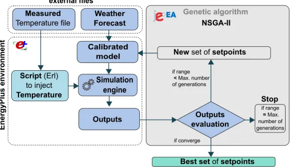
Figure1shows the optimization process. It is divided in two parts: the simulation environment (left side) and the algorithm in charge of the optimization process (right side).
• Simulation environment. As explained in Section1, building energy models play an important role in the process of obtaining good MPC solutions. The optimization process evaluates the outputs of the model in each iteration, so the more accurate the results, the better the evaluation. EnergyPlus software [11] is used to perform the simulations due to the proven quality of its results, which is perhaps why it is one of the most commonly used applications to perform detailed simulations [46]. The methodology starts with the use of calibrated energy models to simulate the behavior of the building. The process to obtain them is described in our latest research on this topic [47–50].
Once the model has been calibrated, it is necessary to reproduce in each simulation all of the aspects that influence the energy model so that the thermal dynamics of the building are not
compromised. That is the reason why the process needs two external files, as can be seen in Figure1: the weather forecast and the file with the measured temperatures of the building’s thermal zones. As Ascione et al. [24] highlight, the accuracy and reliability of weather forecasts is one of the main critical issues for MPC optimizations since inaccuracies greatly affect the simulation results. Secondly, the measured temperature file is needed to solve the EnergyPlus initialization issue described by many authors [17,19,22,51]. The software performs several warm-ups prior to the simulation in order to establish a temperature convergence in the thermal zone. These warm-ups can produce distortions in the results of MPC because, for a specific time horizon, all the simulations should be initialized with the same values. Thanks to a specific script developed in ERL (EnergyPlus Runtime Language), it is possible to inject the measured temperatures, ensuring that the model has the thermal dynamics captured before MPC process starts. Thus, the behavior of the calibrated detailed model is the most accurate possible.
Once the model is defined, the simulation gives us the objectives (outputs) that the optimization algorithm needs to evaluate the proposed solution. In this case, different temperature set-points (solutions) are evaluated through energy consumption minimization. These solutions could be used, for instance, in a real building scenario for day-ahead approaches. The choice of this cost function is explained in Section2.2, but others could have been chosen (predicted mean vote (PMV), use of renewable energy, evaluation of energy and demand cost, and so on).
Finally, it is important to highlight that detailed energy models have computational time as a major disadvantage. This is a critical issue due to the fact that the optimization process needs to run a high number of simulations in each iteration. To solve this issue, it is necessary to act on two fronts, improving hardware capabilities and correcting and adjusting the simulation file. The former is due to features such as clock speed and the number of computer cores are very important since they affect the simulation time and the number of parallel jobs that can be performed, respectively. The latter can result from incorrect run periods, unused elements (such as schedules, materials, constructions and loads), modeling inefficiencies (including a high number of shading surfaces and useless computed outputs), among others, stacked against the simulation time. All these key points should be checked before running the optimization process. • Optimization engine (genetic algorithm). The software used to perform the optimization
is JEplus+EA [52]. The algorithm that this software uses is a genetic algorithm called a non-dominated sorting genetic algorithm II (NSGA-II) [53]. It is an evolutionary algorithm based on the Darwin’s Theory of Evolution, where a population of individuals is evolved generation after generation. The user defines the size of the population and the number of generations. In the optimization process, the algorithm takes advantage of different strategies to prevent solutions falling into a local minimum, thanks to the simulated binary crossover (SBX) and polynomial mutation, and to reduce the time needed to converge, obtaining good solutions in less time using the non-dominated sorting of the population. It is one of the most commonly used algorithms to perform optimizations [46]. As it is a stochastic process, the algorithm has to perform many simulations before reaching an optimal solution and it cannot be guaranteed that the algorithm finds good solutions in a specific simulation time, but, as will be seen in the following sections, the accuracy ratio is very high. When the search space is too large and the simulation time is not enough, the algorithm could carry out unfeasible results. To avoid that, in this paper, we present a two-stage strategy where the algorithm will be performed twice with a different level of accuracy. This strategy allows a faster convergence to a solution than the one-stage strategy and it will be explained and discussed in detail in the case study section.
The objective function is another key element of the optimization process. In this methodology, the convergence towards the free oscillation curve that is obtained through the heating/cooling energy demand of the HVAC system is selected. This way, it is possible to test the accuracy of the algorithm during the optimization process. This is because the free oscillation curve offers a unique solution of zero energy consumption. The uniqueness of the solution allows us to verify
the performance of the algorithm in both aspects: the convergence time and accuracy in the proposed solution. The results of this test can be extrapolated to other optimization problems.
EnergyP lus environment Measured Temperature file Script(Erl) to inject Temperature Weather Forecast
Simulation
engine
external files
Genetic algorithmNewset of setpoints
Outputs evaluation
NSGA-II
Best setof setpoints Calibrated model if range <Max. number of generations if converge Stop if range =Max. number of generations Outputs
Figure 1.Model Predictive Control (MPC) general optimization schema. 2.2. Search Space Reduction Strategy
The search space reduction is an important issue that has been addressed by other authors previously [23,26]. It has a direct relationship with the optimization time, and, when working with detailed energy models, the dimension of the search space should be controlled in order to produce feasible results in time. In the present case, a stochastic algorithm was selected (NSGA-II). This kind of algorithm can work with discrete values in which it is easier to control the search space. In contrast, deterministic algorithms, such as the discrete Armijo gradient algorithm, which require smoothness in the cost function and it has to work with continuous values because it is very sensitive to discontinuities. In that case, the control of the search space is more complex and accordingly it is not recommended to use this algorithm for EnergyPlus optimization problems [54]. For this reason, finite search spaces (those formed by discrete values) are better than infinite search spaces (those formed by continuous values). That is why “the use of discrete variables is very popular in building performance optimization because it speeds up the optimization algorithm convergence and makes the procedure more realistic” as Ascione et al. explain [24,25].
This is closely related to the way a building’s HVAC system works because it does not make sense to have a thermostat set-point with several decimals or to compute two set-points with a difference between them of 0.01◦C. Thus, it is reasonable to use integer values, even float type values with one decimal place and rounded to half or a quarter degree Celsius. This decision is reinforced by the fact that, generally, the accuracy of building’s thermostats is half a degree.
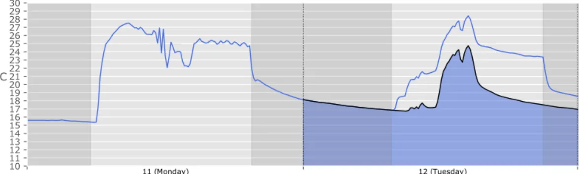
In addition, the methodology described in this article takes advantage of the free oscillation temperature of each thermal zone in order to reduce the search space. The free oscillation curve (FOC) represents the line of zero energy consumption, where the HVAC systems are off. There is no reason to compute solutions (temperature set-points) under the free oscillation curve in winter, or above it in summer. As an example, Figure2shows the measured temperature (blue line) and the free oscillation curve (black line) of thermal zone TZ14 of the case study. The shadowed blue area in Figure2represents all the set-points that have no sense to compute. This implies a significant reduction in the search space, resulting in savings in the computing time for the solution. It is worth highlighting that the accuracy of the FOC will depend on the accuracy of the model and the weather forecast.
10 11 12 13 14 15 16 17 18 19 20 21 22 23 24 25 26 27 28 29 30 11 (Monday) 12 (Tuesday) ºC
Figure 2.Measured temperature (blue line) and free oscillation temperature (black line) of thermal zone 14. Office building, School of Architecture (University of Navarra), 11–12 December 2017.
3. Case Study
In this section, the main components of the case study are stated. 3.1. Building Energy Model Description
This methodology has been tested using a case study, the office building of the School of Architecture of the University of Navarra in Pamplona, Spain (see Figure3), designed by the architects Carlos Sobrini, Rafael Echaide and Eugenio Aguinaga. This building of the 1970s is characterized by the use of simple materials (red bricks, simple-pane windows, concrete pillars, etc.). The façade is composed of two layers of brick 12 cm thick (interior and exterior) and with an insulation of mineral wool inside the chamber. The roof is formed (from inside to outside) by a dropped ceiling, concrete slab (30 cm), a waterproofing membrane, expanded polystyrene (EPS) foam insulation (12 cm), geotextile membranes and gravel (20 cm). The windows are simple-pane without a thermal bridge break. The building is protected from the wind by the School of Architecture on the north side and by a wall of red bricks in all the other orientations. It is fully monitored with temperature sensors in all the spaces (Onset-HOBO ZW-006 with TMC6-HD, TMC20-HD and TMC50-HD (Onset, Cape Cod, Massachusetts, US)), non-invasive sensors (YHDC SCT013 (Beijing Yaohuadechang Electronic CO LTD, China)) for the electric radiators and an energy meter (Kamstrup Multical 602, (Kamstrup A/S, Skamderborg, Central Jutlandia, Denmark)).
Figure 3.Office building, School of Architecture (University of Navarra).
The calibrated model has been realized using OpenStudio (v. 2.6.0) and EnergyPlus software (v. 8.9) [11,55]. Figure4shows different views of the model (by surface type and thermal zone) and the 25 thermal zones into which the building energy model (BEM) is divided, where the colors represent the uses of the different thermal zones. The entire model has a surface of 755.04 m2.
Figure 4.OpenStudio model of the office building (School of Architecture), University of Navarra. (left upper corner): render by surface type, (left lower corner): render by thermal zone, right: thermal zones and space types in the building energy model.
To test the methodology, real weather data for the year 2017 taken from an in situ weather station was used (Data Logger Hobo RX3003 (Onset, Cape Cod, MA, USA), Temperature/Relative Humidity Smart Sensor S-THB-M002 (Onset, Cape Cod, Massachusetts, USA), pluviometer S-RGF-M002 (Onset, Cape Cod, MA, USA), ultrasonic anemometer AO-WDS2E (HongYuv Technologies Co., Ltd., Chengdu, Sichuan, China) and a sunshine sensor BF5-SYS (Delta-T devices Ltd., Cambridge, UK)). For the temperature data of each thermal zone, the Onset-HOBO network of around 40 sensors provided the information. The selected day for performing MPC was 12 December 2017 because it was a very cold day after a week with three public holidays and the building had a very high energy demand. Figure5 shows a calendar where the blue color represents the selected MPC day and the light blue color the days of thermal history needed to ensure that the model has captured its own thermal dynamic. Other studies like that developed by May-Ostendorp et al. [23] run the model through a period of a week to preserve the thermal history of the building; Corbin et al. [14] analyze the number of days that the energy model needs to stabilize its loads, highlighting that similar analysis “must be conducted to establish the length of thermal history required by each model”. In our case study, due to the previous public holidays, two weeks have been selected.
Monday Tuesday Wednesday Thursday Friday Saturday Sunday
27
28
29
30
1
2
3
4
5
6
7
8
9
10
11
12
13
14
15
16
17
18
19
20
21
22
23
24
25
26
27
28
29
30
31
December 2017
Figure 5.Selected day for the model predictive control (MPC) case study (blue color), with thermal history indicated in light blue.
3.2. Model Predictive Control Optimization Parameters
As previously stated, the objective for the MPC optimization is to obtain the temperature set-points in a day-ahead time horizon (12 December 2017). In this case study, the computed time horizon is divided into blocks of one hour, so the number of samples for each solution is 24 values. Increasing
the number of samples for each solution implies an increase in the computational complexity of the optimization and, for buildings’ MPC approaches, an hour of time resolution is enough to obtain significant energy savings. As Afram et al. explain, there are fast-moving processes (airflow rate, water flow rate, etc.) and slow-moving processes (air and water temperature) in HVAC systems, and for slow-moving processes hourly data is the “appropriate temporal resolution to capture the process dynamics correctly” [9].
Another way of reducing computational time is by using discrete values for each set-point. As explained in Section2, discrete values are chosen for each hour of the day. A degree-granularity of half a degree is selected for each value in the time horizon solution. As shown in the following sections, the number of elements in this degree-granularity is a key point when the reduction of the search space is at stake.
The last important point to test an MPC optimization is the simulation time. We have performed the simulations using two computers: a standard computer and a workstation. The standard computer has an AMD Ryzen 1700X processor (GlobalFoundries, Chengdu, China) (16 threads, clock speed: 3.4 GHz) with 16 GB of RAM, and the workstation has two Intel Xeon Gold 6148 (Intel, Hillsboro, OR, USA) (40 threads, clock speed: 2.4 GHz) with 96 GB of RAM. The first one needs an average of 1 m:35 s to perform 16 simulations, and the second 2 m:21 s for 40 simulations. The clock speed of the processor is responsible for this time difference, but the number of simultaneous simulations in the workstation is considerably higher.
The next sections analyze the time difference in using both a standard computer and a workstation, the impact that supposes the search space reduction by using the free oscillation of each thermal zone, the influence of degree-granularity and finally other strategies to reduce the optimization time by using two stages in the optimization process of the MPC.
4. Analysis Procedure of the Case Study and Results
The aim of this section is to analyze how to solve the challenges detailed in Section2by using the BEM described in the previous section. To do so, several experiments are performed in order to show the difficulties and the solutions proposed when working with a detailed energy model in an MPC environment. These experiments show how the convergence time of the algorithm and accuracy of the MPC process can be measured. The approach of these experiments is based on the opportunity offered by the free oscillation curve as a known and unique solution. We measure the capacity of the algorithm to find that solution and this measurement then can be extrapolated to other possible MPC problems in order to have a reference case.
4.1. Measuring the Accuracy of the MPC Solutions
In relation to the accuracy of the obtained solutions, the root mean square error (RMSE) has been selected. TheRMSEis an uncertainty index that measures the spread of the data, the residuals with respect to the objective line, being also sensitive to outliers. These residuals measure the difference in degrees between the predicted values and the objective ones (the free oscillation). Equation (1) shows theRMSEformula, wherenis the number of observations (number of samples of the time horizon), andyi−yˆiis the difference between the values of the objective function in degrees (the free oscillation curve) and the obtained MPC solution in each momenti, respectively. LowerRMSEvalues mean there is a better fit with the target. For MPC optimization problems, a value lower than one degree has been considered suitable: RMSE= [1 n n
∑
i=1 (yi−yˆi)2] 1 2. (1)4.2. Convergence Time Test; Free Oscillation Curve Approach
In this section, we seek to show how the search space affects the convergence time of the algorithm when working with a detailed energy model in an MPC optimization environment. To achieve this,
we consider two experiments. In the first, the free oscillation curve is in the middle of a set of values (Figure6). The distance between each line is 0.5◦C. An upper/lower limit of 4.5◦C is considered, respectively. The time horizon will always be 24 h, which makes a search space of 1924 =4.89×1030. In the second experiment, the evaluation of set-point values under the free oscillation curve (winter) has no physical sense; therefore, these points can be eliminated from the search space, generating a reduced optimization problem of 1024, as can be seen in Figure6.
0: 00 1: 00 2: 00 3: 00 4: 00 5: 00 6: 00 7: 00 8: 00 9: 00 10: 00 11: 00 12: 00 13: 00 14: 00 15: 00 16: 00 17: 00 18: 00 19: 00 20: 00 21: 00 22: 00 23: 00 10 11 12 13 14 15 16 17 18 19 20 21 22 23 24 25 26 27 28 29 30
free oscillation
19 10 24 24 ºCFigure 6.Search space reduction that supposes the consideration of the free oscillation curve in the winter season. In both experiments, the MPC optimization is performed as a multi-zone optimization because the use of the free oscillation curve has been done in each thermal zone. In other cases, an approach of using the average temperature of all thermal zones can be considered and, based on the authors’ previous tests, similar results will be obtained.
In Figure7, the first experiment, with a search space of 1924possibilities, is analyzed. This scenario was tested with both computers, the standard and the workstation. The genetic algorithm NSGA-II is configured with 200 generations of 16 individuals for the standard computer and 80 generations of 40 individuals for the workstation, depending on the number of threads. Both configurations perform around 3200 simulations because, in each generation, the software (jEPlus + EA v.1.7.7 [56]) does not duplicate elite solutions. Thex-axis (abscissa) of Figure7shows the time and they-axis (ordinate) calculates theRMSEfrom each vector (in degrees). Each blue dot represents the simulation of one possible solution, and, when the solution has anRMSEbelow 1◦C (horizontal dashed line), the blue dot changes to red. This allows the user to identify easily when the algorithm is obtaining reasonably good solutions. The optimization performed by the standard computer is at the top of Figure7and the workstation is at the bottom. As can be seen in both figures, the blue dots are grouped in vertical lines of 16 or 40 individuals. This is how the algorithm evolves the initial population over time, from generation to generation.
In both figures, it is observed how the first populations have highRMSEvalues, and that their reduction in time is very slow; only after 4 h and 20 min of optimization is a solution below the limit of 1◦C found (indicated by the arrow), and only with the standard computer. It is obvious that, with this size of search space and with this strategy, it is difficult to obtain good results in a reasonable time.
RMSE
Figure 7.First experiment: MPC results without free oscillation curve consideration for search space reduction (standard computer (top) and workstation (bottom)).
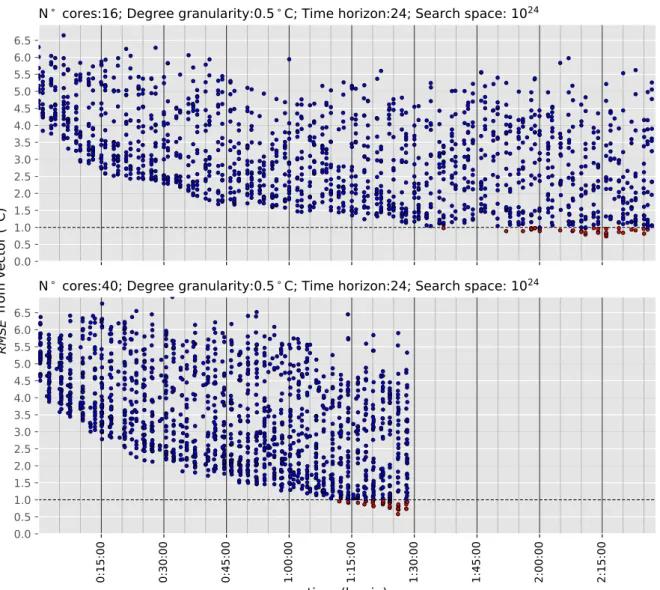
In Figure8, the second experiment with a search space of 1024possibilities is analyzed. As the MPC optimization has a lower search space, 100 generations have been selected for the standard computer and only 40 for the workstation, performing around 1600 simulations each. To prove the robustness of the methodology, these MPC optimizations were performed five times with each computer, the results of Figure8being some of them.
The results obtained with this search space reduction are very significant on both the lower values of theRMSEand the time needed to obtain them. As can be seen, the rhythm of the convergence time of the algorithm is very high, finding enough solutions with anRMSEbelow 1◦C (red dots) in less than half the time previously required. However, as it shows, the reduction in time that supposes the use of the workstation computer is overwhelming, obtaining solutions withRMSEvalues near 0.5◦C in less than 1.5 h. For this reason, from now until the end of this paper, all of the MPC optimizations were performed with the workstation. This simple experiment allows us to understand the importance of considering the free oscillation curve in MPC optimization problems, since it can drastically reduce both the search space and the convergence time of the algorithm. The confidence in the search space reduction of the free oscillation curve is based on the idea of having a high-fidelity calibrated model
that complies with international standards of calibration (ASHRAE 14-2014 Guidelines [57], M&V Guidelines [58] and International Performance Measurement and Verification Protocol (IPMVP) [59]). The authors have developed different techniques in previous articles in order to achieve these kinds of models [47–50].
RMSE
Figure 8.Second experiment: MPC results with free oscillation curve consideration for search space reduction (standard computer (top) and workstation (bottom)).
4.3. Search Space Reduction; Two Stages Process Approach
Most applications that need MPC optimizations (demand response [60], energy flexibility studies, etc.) have challenging computational times, in general below one hour [21]. As shown in the previous section, the search space reduction that is supposed to work with the free oscillation curve is not enough to reach this range, so it is necessary to look for a solution that can reduce the convergence time.
The proposed solution is to perform the MPC optimization in two stages: the first with a degree-granularity of 1◦C and the second with 0.5◦C. Both stages are dependent, as the second stage begins with the best optimization results obtained in the first. The benefits of this approach are substantial: first because the search space in each stage is smaller, which is positive for the genetic algorithm; secondly, because it decreases the convergence time of the algorithm by controlling in two stages the sensitivity of each parameter of the MPC solution; and finally, as the same accuracy is obtained with a significant reduction in time, consequently ensuring the optimization does not lose accuracy in the process.
In this case, to make the test more realistic compared to a real MPC optimization, the values of the free oscillation curve have not been included in the first stage as a possible option. This means that the best solution will never be reached in the first stage; a real case will probabilistically be more favorable and better results could be obtained.
Figure9shows the optimization results obtained using these two stages across a 24-h time horizon. The left side of the figure represents the first stage and the right side the second stage, where 35 min was chosen as the time limit for the former. The darker zones on both sides represent the best solution that can be achieved in each stage. As has been noted, as the free oscillation values are not included in the first stage, the lower possible value for theRMSEis 1◦C. In contrast, in the second stage, the darker zone represents the minimum error of the best solution achieved in the first stage (indicated by an arrow). In this case, the best solution of the first stage has anRMSEof 0.118◦C, which is the height of the darker zone on the right side (the second stage). The results in Figure9show many solutions from the 40th min and the accuracy at the end is near 0.5◦C ofRMSE. Thus, it is demonstrated that the approach is valid; the accuracy of the results obtained are similar to those obtained in Figure8and there is a convergence time reduction of more than 25 min.
RMSE error: 0.118 (°C)
FIRST STAGE SECOND STAGE
RMSE
Figure 9.MPC results using two stages to obtain the MPC vector (24 h).
However, sometimes the MPC optimization needs to be performed in lower time horizons. In these cases, there are fewer parameters to optimize in the MPC solution and hence the time needed is lower. Figure10shows an MPC optimization of 16 h with a first stage of only 20 min. From the 35th minute to the end, there are many solutions, with theRMSEnear 0.5◦C.
FIRST STAGE SECOND STAGE
RMSE error: 0.172 (°C)
RMSE
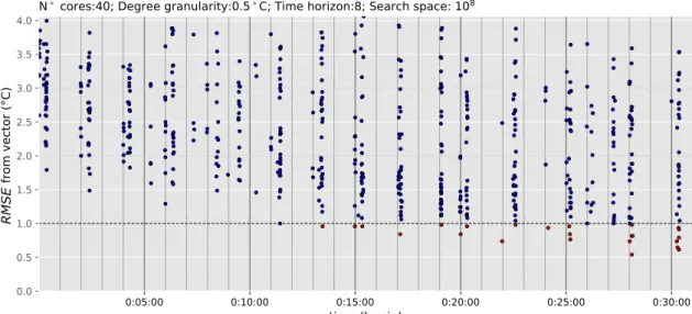
Finally, Figure11shows an MPC optimization across an 8-h time horizon. Here, the search space is very small, but, unlike the previous cases, the algorithm does not have enough time to evolve the population and obtain feasible solutions. It finds only one solution with anRMSEbelow 1◦C in the 24th min.
RMSE
RMSE error: 0.457 (°C)
FIRST STAGE SECOND STAGE
Figure 11.MPC results using two stages to obtain the MPC vector (8 h).
With small search spaces, it is not worth it to perform two stages because the number of generations is divided between them and hence there is not enough time to converge. In these cases, the normal approach of one stage is enough, as can be seen in Figure12, where the algorithm starts finding solutions from the 15th min.
RMSE
Figure 12.MPC results using one stage to obtain the MPC vector (8 h). 4.4. Energy Balance Using the Different Strategies
Table1summarizes the implication of the different MPC strategies in terms of energy. Firstly, an optimal model has been defined. In this case, we have assumed a model with all the set-points fixed at 21◦C that will serve us as our baseline model. Then, all the MPC errors obtained with the different strategies have been applied to this model. In order to analyzed the error in terms of energy, theRMSEerror (◦C), the energy (kWh) and its percentage with respect to the baseline model have been evaluated in three cases: without free oscillation, with free oscillation in one stage and with free oscillation in two stages.
Table 1.Energy balance after applying the different strategies to the real case study.
Time Limit
Without Free Oscillation With Free Oscillation
One Stage (Figure7) One Stage (Figure8) Two Stages (Figure9) RMSE(◦C) Energy (kWh) % RMSE(◦C) Energy (kWh) % RMSE(◦C) Energy (kWh) %
2 h:30 min 0.559 353.18 8.27% - - -
-1 h:30 min 0.559 353.18 8.27% 0.289 335.79 3.52% - -
-1 h:00 min 0.586 353.48 8.35% 0.637 359.99 10.01% 0.368 336.45 3.71% Energy from the optimum solution (baseline model): 326.53 kWh
In the first case, the solutions obtained using a standard MPC (without free oscillation) are very homogeneous in their energy demand (Table1). The search space is so large that the algorithm does not have enough time to evolve the population and obtain good results (see Figure7); in fact, the best solution found within a 2.5 h limit is the same as within 90 min. In the second case, the solutions obtained taking into account the free oscillation have a reduction of search space sufficient that its evolution in time is very fast (see Figures8and9). In the case of one stage optimization, the solution found within 1 h limit is a bit worse than the one obtained with the entire search space. The reason for that is, as is a stochastic optimization, the algorithm generates random solutions that sometimes need more time to converge. However, as can be seen, within a 90 min limit, the evolution of the optimization with this strategy improves, finding a solution that only differs from the optimum one by 3.52%. In the third case, the reduction in time is important, obtaining very good solutions in less than an hour. In this case, the solution was found in the 55th minute and only represents an increase in energy demand of 3.71% (9.92 kWh) with respect to the optimum. This is the main novelty of this paper and implies that, with this strategy, it is possible to comply with the limits recommended by Hedegaard et al. [21] to perform MPC optimizations.
5. Conclusions and Future Research
The main objective of all model predictive control approaches is to obtain future solutions for a problem based on actual and future data performed by a model. These solutions should be provided within a reasonable time and to a certain level of quality. In this context, an MPC optimization with a detailed energy model has been performed. A novel methodology to measure the convergence time and accuracy of the solution has been demonstrated through a specific case study. These values can be extrapolated to other similar problems where an optimal curve of set-points is sought.
The accuracy and convergence time have been tested in different time horizons (24, 16 and 8 h) thanks to a novel technique based on the free oscillation curve. In the cases of 24 and 16 h, a novel two-stage strategy has been performed with a significant reduction in time. In the case of the 8-h time horizon, it has not been necessary to perform a two-stage strategy to obtain good results. For that reason, 8 h can be considered the maximum time horizon that could be performed within a one-stage strategy.
The reduction of the search space can be considered another novel element of the methodology. Genetic algorithms need to control the search space in order to offer reliable solutions in time. Therefore, the computation of continuous values could carry the algorithm to unfeasible results. In this case, we have considered discrete values with a difference between them of 0.5◦C, specified as the granularity limit. The reason is that most thermostat errors are within that margin and lower values would only increase the search space without a significant improvement in the optimal curve. On the other hand, the introduction of the free oscillation curve in the computation of possible set-points for evaluation permits a reduction in the search space because this curve allows the elimination set-point values that have no physical sense and therefore should not be computed.
The approach of using detailed energy models, which have parameters with a physical sense, could extend this model predictive control optimization for many experts within the energy sector because these models could be available in many stages of the life cycle of a building. Alternatively,
when working with detailed energy models, real data from the building management system can easily be integrated in the optimization process. In contrast, simplified models, where the parameters have no physical sense, should be handled by experts with specific knowledge, thereby increasing the level of complexity [14].
This methodology should be performed in real test case studies where the results of the prediction should be confirmed with the data gathered from the meters in the real building.
Author Contributions:G.R.R. has written the manuscript, developed the scripts and performed the simulations; E.L.S. has supervised the Model Predictive Control concept; C.F.B. has developed the methodology that has been proposed in the article; All the authors have revised and verified all the manuscript before sending it to the journal.
Funding:This research was funded by the Government of Navarra under the project SYMMETRI (ref. PC010-011). Acknowledgments:We would like to thank the School of Architecture of the University of Navarra for coexisting with a monitored building, in particular to those staff who work in the office area, and to the Welsh School of Architecture of Cardiff University for hosting the stay of the researcher Carlos Fernández Bandera. Additionally, we highlight that the monitorization has been realized thanks to funding received from a research project granted by the Government of Navarra (SYMMETRI—“smart campus: electro-thermal microgrid”). Finally, we would like to thank Saviarquitectura Research Group for the equipment loans (workstation).
Conflicts of Interest:The authors declare no conflicts of interest.
Abbreviations
The following abbreviations are used in this manuscript:
ABC Artificial Bee Colony
ANN Artificial Neural Network
ASHRAE American Society of Heating, Refrigerating, and Air-Conditioning Engineers
BEM Building Energy Model
EPBD Energy Performance of Buildings
ERL EnergyPlus Runtime Language
FOC Free Oscillation Curve
GA Genetic Algorithm
HVAC Heating Ventilation and Air-Conditioning
IPMVP International Performance Measurement and Verification Protocol
MPC Model Predictive Control
NSGA Non Sorting Genetic Algorithm
PCM Phase Change Material
PID Proportional-Integrative-Derivative)
PMV Predicted Mean Vote
PPD Predicted Percentage Dissatisfied
PVT Photovoltaic-Thermal System
RC Resistance Capacitance
RMSE Root Mean Square Error
SBX Simulated Binary Crossover
SVM Support Vector Machine
References
1. Directive, E.E. Directive 2012/27/EU of the European Parliament and of the Council of 25 October 2012 on energy efficiency, amending Directives 2009/125/EC and 2010/30/EU and repealing Directives 2004/8/EC and 2006/32. Off. J. L2012,315, 1–56.
2. European Commission. Proposal for a Directive of the European Parliament and of the Council amending Directive 2012/27/EU on energy efficiency COM/2016/0761 Final—2016/0376 (COD); European Commission: Brussels, Belgium, 2016.
3. Fraunhofer, I.How Energy Efficiency Cuts Costs for a 2-Degree Future; Fraunhofer Institute for Systems and Innovation Research ISI: Karlsruhe, Germany, 2015.
4. EPBD. Directive 2002/91/EC of the European Parliament and of the Council of 16 December 2002 on the energy performance of buildings. Off. J. Eur. Union2002,1, 65–71.
5. Recast, E. Directive 2010/31/EU of the European Parliament and of the Council of 19 May 2010 on the energy performance of buildings (recast). Off. J. Eur. Union2010,18, 2010.
6. Peeters, L.; Van der Veken, J.; Hens, H.; Helsen, L.; D’haeseleer, W. Control of heating systems in residential buildings: Current practice. Energy Build.2008,40, 1446–1455. [CrossRef]
7. Braun, J.E. Reducing energy costs and peak electrical demand through optimal control of building thermal storage.ASHRAE Trans.1990,96, 876–888.
8. Liao, Z.; Dexter, A. The potential for energy saving in heating systems through improving boiler controls. Energy Build.2004,36, 261–271. [CrossRef]
9. Afram, A.; Janabi-Sharifi, F. Theory and applications of HVAC control systems—A review of model predictive control (MPC).Build. Environ.2014,72, 343–355. [CrossRef]
10. Serale, G.; Fiorentini, M.; Capozzoli, A.; Bernardini, D.; Bemporad, A. Model predictive control (MPC) for enhancing building and HVAC system energy efficiency: Problem formulation, applications and opportunities. Energies2018,11, 631. [CrossRef]
11. Crawley, D.B.; Lawrie, L.K.; Winkelmann, F.C.; Buhl, W.F.; Huang, Y.J.; Pedersen, C.O.; Strand, R.K.; Liesen, R.J.; Fisher, D.E.; Witte, M.J.; et al. EnergyPlus: creating a new-generation building energy simulation program. Energy Build.2001,33, 319–331. [CrossRef]
12. Trnsys, A.Transient System Simulation Program; University of Wisconsin: Madison, WI, USA, 2000. 13. Li, X.; Wen, J. Review of building energy modeling for control and operation. Renew. Sustain. Energy Rev.
2014,37, 517–537. [CrossRef]
14. Corbin, C.D.; Henze, G.P.; May-Ostendorp, P. A model predictive control optimization environment for real-time commercial building application. J. Build. Perform. Simul.2013,6, 159–174. [CrossRef]
15. Kwak, Y.; Huh, J.H.; Jang, C. Development of a model predictive control framework through real-time building energy management system data.Appl. Energy2015,155, 1–13. [CrossRef]
16. Li, X.; Malkawi, A. Multi-objective optimization for thermal mass model predictive control in small and medium size commercial buildings under summer weather conditions. Energy2016, 112, 1194–1206. [CrossRef]
17. Coffey, B.; Haghighat, F.; Morofsky, E.; Kutrowski, E. A software framework for model predictive control with GenOpt. Energy Build.2010,42, 1084–1092. [CrossRef]
18. Reynolds, J.; Rezgui, Y.; Kwan, A.; Piriou, S. A zone-level, building energy optimisation combining an artificial neural network, a genetic algorithm, and model predictive control. Energy2018,151, 729–739. [CrossRef]
19. Zakula, T.; Armstrong, P.R.; Norford, L. Modeling environment for model predictive control of buildings. Energy Build.2014,85, 549–559. [CrossRef]
20. Péan, T.Q.; Salom, J.; Costa-Castelló, R. Review of control strategies for improving the energy flexibility provided by heat pump systems in buildings. J. Process Control2018, in press.
21. Hedegaard, R.E.; Pedersen, T.H.; Petersen, S. Multi-market demand response using economic model predictive control of space heating in residential buildings.Energy Build.2017,150, 253–261. [CrossRef] 22. Henze, G.P.; Krarti, M.Predictive pOtimal Control of Active and Passive Building Thermal Storage Inventory;
Technical Report; University Of Nebraska: Lincoln, NE, USA, 2005.
23. May-Ostendorp, P.; Henze, G.P.; Corbin, C.D.; Rajagopalan, B.; Felsmann, C. Model-predictive control of mixed-mode buildings with rule extraction. Build. Environ.2011,46, 428–437. [CrossRef]
24. Ascione, F.; Bianco, N.; De Stasio, C.; Mauro, G.M.; Vanoli, G.P. Simulation-based model predictive control by the multi-objective optimization of building energy performance and thermal comfort. Energy Build. 2016,111, 131–144. [CrossRef]
25. Ascione, F.; Bianco, N.; De Stasio, C.; Mauro, G.M.; Vanoli, G.P. A new comprehensive approach for cost-optimal building design integrated with the multi-objective model predictive control of HVAC systems.Sustain. Cities Soc.2017,31, 136–150. [CrossRef]
26. Coffey, B. A Development and Testing Framework for Simulation-Based Supervisory Control With Application to Optimal Zone Temperature Ramping Demand Response Using a Modified Genetic Algorithm. Ph.D. Thesis, Concordia University, Montreal, QC, Canada, 2008.
27. Henze, G.; May-Ostendorp, P. HVAC Control Algorithms for Mixed Mode Buildings. InUS Green Building Council Green Building Research Fund Final Report; CRC Press: Boca raton, FL, USA, 2012; Volume 133. 28. Moon, J.W.; Kim, K.; Min, H. ANN-based prediction and optimization of cooling system in hotel rooms.
Energies2015,8, 10775–10795. [CrossRef]
29. Afram, A.; Janabi-Sharifi, F.; Fung, A.S.; Raahemifar, K. Artificial neural network (ANN) based model predictive control (MPC) and optimization of HVAC systems: A state of the art review and case study of a residential HVAC system.Energy Build.2017,141, 96–113. [CrossRef]
30. Paris, B.; Eynard, J.; Grieu, S.; Talbert, T.; Polit, M. Heating control schemes for energy management in buildings. Energy Build.2010,42, 1908–1917. [CrossRef]
31. Killian, M.; Kozek, M. Implementation of cooperative Fuzzy model predictive control for an energy-efficient office building.Energy Build.2018,158, 1404–1416. [CrossRef]
32. Feng, K.; Lu, J.; Chen, J. Nonlinear model predictive control based on support vector machine and genetic algorithm. Chin. J. Chem. Eng.2015,23, 2048–2052. [CrossRef]
33. Širok `y, J.; Oldewurtel, F.; Cigler, J.; Prívara, S. Experimental analysis of model predictive control for an energy efficient building heating system. Appl. Energy2011,88, 3079–3087. [CrossRef]
34. Huang, H.; Chen, L.; Hu, E. A new model predictive control scheme for energy and cost savings in commercial buildings: An airport terminal building case study. Build. Environ. 2015, 89, 203–216. [CrossRef]
35. Bruni, G.; Cordiner, S.; Mulone, V.; Sinisi, V.; Spagnolo, F. Energy management in a domestic microgrid by means of model predictive controllers. Energy2016,108, 119–131. [CrossRef]
36. Oldewurtel, F.; Parisio, A.; Jones, C.N.; Gyalistras, D.; Gwerder, M.; Stauch, V.; Lehmann, B.; Morari, M. Use of model predictive control and weather forecasts for energy efficient building climate control. Energy Build.2012,45, 15–27. [CrossRef]
37. Carrascal, E.; Garrido, I.; Garrido, A.J.; Sala, J.M. Optimization of the heating system use in aged public buildings via model predictive control. Energies2016,9, 251. [CrossRef]
38. Fiorentini, M.; Wall, J.; Ma, Z.; Braslavsky, J.H.; Cooper, P. Hybrid model predictive control of a residential HVAC system with on-site thermal energy generation and storage. Appl. Energy2017,187, 465–479. [CrossRef]
39. Chen, L.; Du, S.; He, Y.; Liang, M.; Xu, D. Robust model predictive control for greenhouse temperature based on particle swarm optimization.Inf. Process. Agric.2018,5, 329–338. [CrossRef]
40. Khanmirza, E.; Esmaeilzadeh, A.; Markazi, A.H.D. Design and experimental evaluation of model predictive control vs. intelligent methods for domestic heating systems. Energy Build.2017,150, 52–70. [CrossRef] 41. Aggelogiannaki, E.; Sarimveis, H. A simulated annealing algorithm for prioritized multiobjective
optimization—Implementation in an adaptive model predictive control configuration. IEEE Trans. Syst. Man Cybern. Part B (Cybern.)2007,37, 902–915. [CrossRef]
42. Ding, L.; Lv, J.; Li, X.; Li, L. Support vector regression and ant colony optimization for HVAC cooling load prediction. In Proceedings of the 2010 International Symposium on Computer, Communication, Control and Automation (3CA), Tainan, Taiwan, 5–7 May 2010; Volume 1, pp. 537–541.
43. Delgarm, N.; Sajadi, B.; Delgarm, S. Multi-objective optimization of building energy performance and indoor thermal comfort: A new method using artificial bee colony (ABC).Energy Build.2016,131, 42–53. [CrossRef]
44. Zhang, X.; Fong, K.F.; Yuen, S.Y. A novel artificial bee colony algorithm for HVAC optimization problems. HVAC&R Res.2013,19, 715–731.
45. Pavlak, G.S.; Henze, G.P.; Cushing, V.J. Evaluating synergistic effect of optimally controlling commercial building thermal mass portfolios.Energy2015,84, 161–176. [CrossRef]
46. Nguyen, A.T.; Reiter, S.; Rigo, P. A review on simulation-based optimization methods applied to building performance analysis.Appl. Energy2014,113, 1043–1058. [CrossRef]
47. Ruiz, G.R.; Bandera, C.F.; Temes, T.G.A.; Gutierrez, A.S.O. Genetic algorithm for building envelope calibration. Appl. Energy2016,168, 691–705. [CrossRef]
48. Ruiz, G.R.; Bandera, C.F. Analysis of uncertainty indices used for building envelope calibration. Appl. Energy2017,185, 82–94. [CrossRef]
49. Ruiz, G.R.; Bandera, C.F. Validation of Calibrated Energy Models: Common Errors. Energies2017,10, 1587. [CrossRef]
50. Fernández Bandera, C.; Ramos Ruiz, G. Towards a New Generation of Building Envelope Calibration. Energies2017,10, 2102. [CrossRef]
51. Machairas, V.; Tsangrassoulis, A.; Axarli, K. Algorithms for optimization of building design: A review. Renew. Sustain. Energy Rev.2014,31, 101–112. [CrossRef]
52. Zhang, Y.; Korolija, I. Performing complex parametric simulations with jEPlus. In Proceedings of the Ninth International Conference on Sustainable Energy Technologies (SET), Shanghai, China, 24–27 August 2010; pp. 24–27.
53. Deb, K.; Pratap, A.; Agarwal, S.; Meyarivan, T. A fast and elitist multiobjective genetic algorithm: NSGA-II. IEEE Trans. Evol. Comput. 2002,6, 182–197. [CrossRef]
54. Wetter, M.; Wright, J. A comparison of deterministic and probabilistic optimization algorithms for nonsmooth simulation-based optimization.Build. Environ.2004,39, 989–999. [CrossRef]
55. Guglielmetti, R.; Macumber, D.; Long, N. OpenStudio: an open source integrated analysis platform. In Proceedings of the 12th Conference of International Building Performance Simulation Association, Sydney, Australia, 14–16 November 2011.
56. Zhang, Y. Use jEPlus as an efficient building design optimisation tool. In Proceedings of the CIBSE ASHRAE Technical Symposium, London, UK, 18–19 April 2012; pp. 18–19.
57. ASHRAE. Guideline 14-2014, Measurement of Energy and Demand Savings; Technical Report; American Society of Heating, Ventilating, and Air Conditioning Engineers: Atlanta, GA, USA, 2014.
58. Webster, L.; Bradford, J.; Sartor, D.; Shonder, J.; Atkin, E.; Dunnivant, S.; Frank, D.; Franconi, E.; Jump, D.; Schiller, S.; et al. M&V Guidelines: Measurement and Verification for Performance-Based Contracts. Version 4.0; Technical Report, U.S. Department of Energy Federal Energy Management Program; U.S. Department of Energy: Columbia, WA, USA, 2015.
59. IPMVP Committee. International Performance Measurement and Verification Protocol: Concepts and Options for Determining Energy and Water Savings, Volume I; Technical Report; Efficiency Valuation Organization: Washington, DC, USA, 2012. Available online:www.evo-world.org(accessed on 22 December 2018). 60. Patteeuw, D.; Henze, G.P.; Helsen, L. Comparison of load shifting incentives for low-energy buildings
with heat pumps to attain grid flexibility benefits. Appl. Energy2016,167, 80–92. [CrossRef]
c
2018 by the authors. Licensee MDPI, Basel, Switzerland. This article is an open access article distributed under the terms and conditions of the Creative Commons Attribution (CC BY) license (http://creativecommons.org/licenses/by/4.0/).