Low-Complexity Compressive Sensing Detection
for Spatial Modulation in Large-Scale
Multiple Access Channels
Adrian Garcia-Rodriguez,
Student Member, IEEE
, and Christos Masouros,
Senior Member, IEEE
Abstract—In this paper, we propose a detector, based on the compressive sensing (CS) principles, for multiple-access spatial modulation (SM) channels with a large-scale antenna base sta-tion (BS). Particularly, we exploit the use of a large number of antennas at the BSs and the structure and sparsity of the SM transmitted signals to improve the performance of conventional detection algorithms. Based on the above, we design a CS-based detector that allows the reduction of the signal processing load at the BSs particularly pronounced for SM in large-scale multiple-input–multiple-output (MIMO) systems. We further carry out analytical performance and complexity studies of the proposed scheme to evaluate its usefulness. The theoretical and simulation results presented in this paper show that the proposed strategy constitutes a low-complexity alternative to significantly improve the system’s energy efficiency against conventional MIMO detec-tion in the multiple-access channel.
Index Terms—Spatial modulation, large-scale MIMO, multiple access, compressive sensing, energy efficiency.
I. INTRODUCTION
T
HE exponential growth of the data rates in wireless com-munications has caused a significant increase in the total energy consumption required to establish the communication links [1]. This is because novel transceiver structures with a higher number of antennas, transmission power or complexity in their signal processing algorithms have been designed to accommodate this growth [1], [2]. For this reason, the energy efficiency (EE) of the multi-user wireless transmission con-stitutes one of the main areas of research interest at present [1], [2]. Technologies such as large-scale MIMO and SM have been developed with the main objective of satisfying the EE re-quirements of future wireless communication systems [3], [4].Massive MIMO technologies increase the EE by incorporat-ing a large number of antennas at the BSs [4]–[7]. This leads to communication systems in which the use of conventional Manuscript received July 14, 2014; revised March 4, 2015; accepted May 8, 2015. Date of publication May 18, 2015; date of current version July 13, 2015. This work was supported in part by the Royal Academy of Engineering, U.K., and in part by EPSRC under Grant EP/M014150/1. The material in this paper was presented in part at the IEEE International Conference on Acoustics, Speech and Signal Processing, Brisbane, Australia, April 2015, and the IEEE International Conference on Communications, London, U.K., June 2015. The associate editor coordinating the review of this paper and approving it for publication was A. Ghrayeb.
The authors are with the Department of Electronic and Electrical Engineer-ing, University College London, London WC1E 6BT, U.K. (e-mail: adrian. [email protected]; [email protected]).
Color versions of one or more of the figures in this paper are available online at http://ieeexplore.ieee.org.
Digital Object Identifier 10.1109/TCOMM.2015.2434817
linear detection and precoding techniques becomes optimal in the large-scale limit [4], [5]. However, the increased number of radio frequency (RF) chains have a considerable influence on the EE, hence severely affecting the large-scale benefits from this perspective [8]. To alleviate this impact, SM poses as a reduced RF-complexity scheme by exploiting the transmit antenna indices as an additional source of information [3], [9]. Intuitively, instead of activating all the antennas simultaneously as in conventional MIMO transmission, SM proposes to switch on a subset of them and modify the receiver’s operation to detect both the active antenna indices and the amplitude-phase symbols. This reduces the number of RF chains when compared to conventional MIMO systems at the cost of decreasing the maximum achievable rates [3], [9], [10].
So far, the literature of SM has mostly focused on de-veloping strategies for point-to-point links [3], [9]–[15]. For instance, several low-complexity detectors that approach the performance of the optimal maximum likelihood (ML) esti-mation have been proposed [15]–[18]. In this context, the use of a normalized CS detection algorithm as a low-complexity solution for space shift keying (SSK) and generalized space shift keying (GSSK) peer-to-peer (P2P) systems was introduced in [18]. In this work, the authors apply a normalization to the channel matrix before the application of the greedy compressive detector to improve performance. However, the authors restrict its application to single-user SSK and GSSK systems, which constrains its use to low data rate transmission. The perfor-mance of the normalized CS detection for SSK and GSSK has been recently enhanced in [19], where the improvement is obtained by pre-equalizing the received signal.
More recently, the use of SM has been extended to the multiple access channel (MAC) as a way of enhancing the achievable rates of the conventional single-antenna devices considered in this setting [20]–[22]. The literature related to the study of multiple access SM builds upon [20], [21], where a characterization of the bit error rate (BER) probabilities of the optimal ML detector for both spatial and SSK modulations is performed. However, the signal processing load of the ML detector makes it impractical in the MAC as it grows exponen-tially with this parameter [20]. In this setting, several detection schemes to reduce the complexity of the ML detector in the MAC have been proposed and studied in [22], where the focus is onQ-ary SSK modulation.
A number of related works have concentrated on the design of detection schemes to account for the particularities of the large-scale MAC. The development of detection schemes in This work is licensed under a Creative Commons Attribution 3.0 License. For more information, see http://creativecommons.org/licenses/by/3.0/
this setting is motivated by the intractable complexity of non-linear detectors such as the sphere decoder when a high number of antennas and users are considered [4], [15]. The use of a message passing detection (MPD) algorithm is proposed in [23] for the MAC with a high number of antennas at the BS. This algorithm offers a performance improvement with respect to conventional MIMO systems with the same spectral efficiency. However, both the storage requirements and the total number of operations are conditioned by the high number of messages transmitted between all the nodes, which must be updated in every iteration [24]. A more complex local search detection algorithm based on finding the local optimum in terms of the maximum likelihood cost is also introduced in [23]. An iterative detector for large-scale MACs is developed in [25]. Here, the authors decouple the antenna and symbol es-timation processes to reduce the global detection complexity. The algorithm introduced in [26] accounts for the sparsity and signal prior probability of SM transmission in the MAC. In this work, the use of stage-wised linear detection is discarded due to its high complexity and the authors propose a generalized approximate message passing detector. A related approach has been developed in [27] to deal with quantized measurements and spatial correlation. Still, the above algorithms do not fully account for the particularities of iterative detection processes and the complexity benefits that can be obtained by leveraging the principles behind CS algorithms.
In this paper we propose a low-complexity detector based on CS for the MAC of SM systems with large-scale BSs. In particular, we show that the signal structure of SM in the MAC can be exploited to provide additional information and improve the performance of the CS algorithms [28], [29]. Moreover, the use of a high number of antennas in the MAC allows us to elim-inate the error floor that greedy CS techniques show in noisy scenarios for practical uncoded BERs [18]. Indeed, contrary to the common CS knowledge, in this paper we show by means of a thorough complexity analysis that the trade-off between complexity and performance is especially favorable for CS-based detection schemes in scenarios with a high number of receive antennas.
Furthermore, in this paper we compare the EE and signal processing (SP) complexity of the proposed strategy with the conventional zero forcing (ZF) and minimum mean square error (MMSE) linear detectors. In particular, we show that the improvements offered by the proposed technique allow enhancing the EE achieved with these detectors while re-ducing their computational complexity. In fact, the detailed complexity analysis leads us to derive interesting conclusions regarding the algorithms that must be used to solve the ZF and MMSE detection problems in large-scale SM-MIMO systems. To summarize, the contributions of this paper can be stated as follows:
• We propose and validate the use of CS-based algorithms as an efficient alternative to recover SM signals under large-scale MIMO conditions. Moreover, we design a CS-based detector specifically tailored for the MAC of SM systems to improve the performance and the EE of the detectors conventionally used for large-scale MIMO.
• As opposed to the previous literature, we perform an analytical characterization of the computational com-plexity of the iterative CS algorithm to determine the conditions in which the use of CS-based detection in SM is especially beneficial.
• We carry out a mathematical analysis of the performance and convergence of the CS greedy algorithms when applied to the proposed large-scale MAC scenario.
• We use the above complexity and performance analyses to characterize the EE of the proposed, which is shown to be superior to that of the existing linear detectors.
II. PRELIMINARIES
A. System Model of the Multiple Access Channel (MAC)
The model considered throughout this paper characterizes the MAC of a multi-user MIMO system comprised ofKmobile stations (MSs) withnt antennas each, and a single BS withN
receive antennas. The total number of antennas allocated at the MSs is denoted asM=K×nt. The behavior of the multiple
access system can be described by
y=Hx+w, (1) wherey∈CN×1is the signal received at the BS, andx∈CM×1 denotes the signal transmitted by the MSs. Moreover, w∈
CN×1∼CN(0, σ2
nIN) denotes the standard additive
white-Gaussian noise vector with variance σn2, and H∈CN×M ∼
CN(0,IN⊗IM)is a matrix whosem,n-th complex coefficient, hm,n, represents the frequency flat fading channel gain between
then-th transmit antenna and them-th receive antenna. In the previous expressions, ∼ indicates “distributed as”, IA is an A×A identity matrix, and ⊗ denotes the Kronecker product [30]. As typically assumed in the SM detection literature, the BS is expected to have a perfect knowledge of the communica-tion channelH[3], [4].
Throughout this paper we assume that the data symbols transmitted by the active antennas belong to a normalized
Q-QAM constellation satisfyingE[Es] =1, whereEs refers to
the symbol energy and the operator E denotes the expected value. Based on this, the total average signal-to-noise ratio (SNR) of the MACρcan be expressed as
ρ= E[xHx] σ2 n = S·E[Es] σ2 n , (2) where(·)H denotes the Hermitian transpose andS≤M is the total number of antennas simultaneously active amongst the MSs.
B. Multiple Access Spatial Modulation
SM and its generalized version reduce the hardware com-plexity of multiple-antenna devices by limiting the number of active antennas per user and conveying additional information onto their spatial position [3], [9]. In this section we focus on describing the operation of generalized SM transmission with a single RF chain since particularization to conventional SM is straightforward by lettingS=K and forcing the number of
antennas per user to be a power of two [9], [31]. Throughout this paper we use the term SM when referring to both conventional and generalized SM for ease of description. In SM, each trans-mitter conveys the same constellation symbol by activating a given number of antennasnaaccording to the input bit sequence
[3], [9], [31]. Without loss of generality, in the following we assume that the users activate the same number of antennas, i.e. we have S=na×K. Mathematically, the transmit
sig-nal xu∈Cnt×1 of the u-th SM transmitter can be expressed
as [9] xu= 0 · · · sql 1 · · · s q lk· · · 0 T , (3) where lk∈ [1,nt] denotes the active antenna index and sq
represents theq-th symbol of the transmit constellationB. The number of bits that can be encoded on the antenna indices is
log2
nt na
[8], [31]. In the previous expression,··denotes the binomial operation and·is the floor function. Therefore, the number of possible antenna combinations at the transmitter is given byr=2b, where blog2nt
na
. This determines the cardinality of A, the set comprised of the possible antenna groups withAlbeing thel-th element. Note that there may be
invalid antenna groups to preserve an integer length of the bit stream. The composite transmit vectorx∈CM×1is obtained by concatenating the transmit signals asx= [xT1xT2· · ·xTK]T.
When compared with conventional MIMO technologies, SM reduces the inter-user interference and the circuit power consumption of the MSs for the same number of antennas. However, this causes a reduction of the achievable rates with respect to conventional MIMO for the same number of antennas [3]. Particularly, while a conventional MIMO transmitter is able to conveyBMIMO=nt·log2(Q)bits, a single SM transmitter encodesBSM=b+log2(Q)bits in every channel use. At the receiver, detection schemes exploit the channel knowledge to determine the active antennas and the conveyed constellation symbols [3]. Among these, the optimum detector follows the ML criterion and its output reads as
ˆ x=arg min ˜ sp y−Hs˜p2 2. (4)
Here, the signal ˜sp∈CM×1 belongs to the set that includes
all the possible transmit signals and · p denotes the p
norm. The cardinality of,|| =(Q×r)K, exponential with the number of users K, establishes an upper bound on the complexity of SM detection.
C. Large-Scale MIMO and Low-Complexity Detection
The large-scale MIMO theory focuses on analyzing the ben-efits of communication systems with a high number of antennas at the BSs [4], [5]. One of the fundamental results in this field states that, provided thatN M, the received signal after linear detectiong∈CM×1satisfies
g=D(Hx+w) −−−−→a.s.
N→∞,M=const.x, (5)
where D∈CM×N is a linear detection matrix that for the
matched filter (MF), ZF and MMSE detectors read as [32] DMF=HH, (6)
DZF=H†=(HHH)−1HH, (7) DMMSE=(HHH+ςI)−1HH. (8) In the above, ς =M/ρ [32], (·)† denotes the pseudoinverse operation and(·)−1refers to the inverse matrix. Letg{u}be the decision vector corresponding to theu-th user. In the following we adopt the sub-optimal but low-complexity approach of decoupling the estimation of the spatial and amplitude-phase modulated symbols [22], [33]. Specifically, the estimated active antenna indicesAˆl and the transmitted constellation symbolqˆ
for theu-th user are obtained from (5) as
ˆ Al=arg max l g{Au} l 2, (9) ˆ q=D g{ˆu} Al , (10) whereg{u} {Al,Aˆl}
represent the entries of the decision vector of the
u-th userg{u} determined by the sets Al andAˆl respectively,
andDdenotes the demodulation function.
Note that the necessary increase in the number of transmit antennas when SM is used degrades the performance of the above-mentioned detectors due to the worse conditioning of the channel matrix. For this reason, in this paper we propose a low-complexity solution inspired by CS to take advantage of the large-scale MIMO benefits while, at the same time, reducing the detection complexity. In other words, in the following we look at scenarios whereN M does not necessarily hold but
N Kbrings the massive MIMO effect.
III. THETRIVIALAPPROACH: DIRECTAPPLICATION OF THECS ALGORITHMS FORSM DETECTION The main issue with the conventional ZF and MMSE linear detectors when applied to SM and generalized SM detection is that the entire channel matrix H∈CN×M must be used for detection even though onlyScolumns contribute to the acquisi-tion of the amplitude-phase signal informaacquisi-tion. We circumvent this by exploiting the sparsity of SM signals to reduce the complexity of linear detectors. The signals conveyed by SM are defined asS-sparse because they only containSM non-zero entries equal to the number of antennas simultaneously active S [18]. This property has been exploited by CS to improve signal estimation from compressive measurements. Specifically, CS capitalizes on signal sparsity to guarantee a reliable signal recovery with efficient algorithms [34], [35]. The CS measurements y∈RN×1 of a sparse signalx can be expressed as [35]–[37]
y=x+e, (11) where x∈RM×1 represents the original sparse signal, ∈
measurement error term. Note that the complex-valued system in (1) can be straightforwardly re-expressed to resemble the real-valued one in (11) [18]. In this paper, we exploit the similarity between (1) and (11) to improve the detection per-formance of the conventional linear MIMO detectors.
In CS, the restricted isometry property (RIP) determines whether signal recovery guarantees are fulfilled or not for any communication channel=H[35], [36]. For the case of the MIMO channel, the RIP of order S is satisfied for a channel matrixHif, for anyS-sparse signalx, the relationships
(1−δS)x22≤ Hx22≤(1+δS)x22 (12) hold for a constantδS∈(0,1). For instance, a matrix comprised
of independent and identically distributed Gaussian random variables is known to satisfy δS≤0.1 provided that N≥ cSlog(M/S), withcbeing a fixed constant [36]. Note that this kind of channel communication matrix conventionally arises in rich scattering environments with Rayleigh fading [4].
Once the signal measurements are acquired and contrary to the ML detector given in (4), the detection of the SM signals in CS relies on the sparsity of SM transmission to generate an estimate. For the case withδ2S<
√
2−1 [37] we solve (4) in a low-complexity CS-inspired fashion as
minimizex1
subject toHx−y2≤μ, (13) In the above expression the constantμlimits the noise power
w2≤μ. Although the above optimization problem can be solved with well-known convex approaches, these alternatives are often computationally intensive, so faster techniques that offer a trade-off between performance and complexity such as greedy algorithms are commonly used instead [36].
From the vast variety of CS greedy algorithms, in this section we choose one of the most efficient schemes to approximate the solution of (13): the Compressive Sampling Matching Pursuit (CoSaMP) [38]. The CoSaMP is a low-complexity algorithm that goes through an iterative reconstruction process to recover both the active antenna indices and the amplitude-phase in-formation of the transmitted signals. Moreover, this algorithm provides optimal error guarantees for the detection of sparse signals since, similarly to the more complex convex algorithms, a stable signal recovery is guaranteed under noisy conditions with a comparable number of receive antennas [38]. In our results we show that the large number of antennas at the BS ben-efits the use of this algorithm for SM detection by performing a thorough complexity analysis as opposed to [18], [38]. More-over, as the structure of the transmitted signals in the MAC is not accounted for in the generic CS detection, in the following we consider an approach specifically tailored for the considered scenarios to improve the detection performance.
IV. PROPOSEDENHANCEDCS TECHNIQUE: SPATIAL MODULATIONMATCHINGPURSUIT(SMMP) One of the key characteristics of the conventional greedy CS algorithms is that no prior knowledge of the sparse signal other
Algorithm 1Spatial Modulation Matching Pursuit Inputs:H,y,S,na,imax.
1:Output:x˜iend S-sparse approximation
2:x˜0←0,i←0 {Initialization} 3:whilehalting criterionfalsedo
4: r←y−Hx˜i {Update residual} 5: i←i+1
6: c←HHr {MF to estimate active antenna indices} {7–11: Detectnaindices with highest energy per user}
7: ←∅
8: forj=1→Kdo
9: M← {(j−1)·nt, . . . ,j·nt−1}
10: ←M(arg max{|c|M|}na)∪
11: end for
{12–13: Detect remainingk−Shighest-energy indices} 12: c()←0
13: ←arg max{|c|}(k−S)∪
14: T ←∪supp(x˜i−1) {Merge supports} 15: b|T ←H†Ty {Least squares problem} 16: b|TC ←0
{17–21: Obtain next signal approximation} 17: x˜i←0
18: forj=1→Kdo
19: M← {(j−1)·nt, . . . ,j·nt−1}
20: x˜i|M(arg max{|b|M|}na)←max{|b|M|}na
21: end for 22:end while
than the number of non-zero entries is assumed. However, when applied to the proposed scenario, this condition can generate situations in which the output of the detector does not have physical sense. For instance, the detected signal could have more than one active antenna per user, which is not possible when conventional SM modulation is used [3]. This undesired operating condition is caused by the noise and inter-user in-terference effects that arise in the MAC. To mitigate these, in this sub-scheme we incorporate the additional prior knowledge about the distribution of the non-zero entries in the transmitted signal to further enhance performance [28].
The detection algorithm considered in this paper is referred to as spatial modulation matching pursuit (SMMP) to explicitly indicate that it corresponds to a particularization to SM op-eration of the structured CoSaMP itop-eration developed in [29]. In particular, SMMP reduces the errors in the identification of the active antennas by exploiting the known distribution of the non-zero entries [28], [29]. This also improves the convergence speed of the algorithm as less iterations are required to deter-mine the active antenna indices. While it is intuitive that the concept behind this strategy could be incorporated to other CS detection algorithms, in the following we focus on the CoSaMP algorithm for clarity.
The pseudocode of the proposed strategy is shown in Algorithm 1 for convenience and its operation can be described as follows [29], [38]. The algorithm starts by producing an estimate of the largest components of the transmitted signal to
identify the active antennas [38]. For this, the algorithm em-ploys the residual signalr∈CN×1given by
ry−Hx˜i=H(x− ˜xi)+w, (14) wherex˜i∈CM×1is the approximation of the transmit signal at thei-th iteration. The residual signal concentrates the energy on the components with a largest error in the estimated received signaly˜=Hx˜i [25], [39]. The decision metric used to deter-mine the plausible active antennasc∈CM×1is obtained as the output of a MF and can be expressed as
c=HHr. (15) From this decision metric, the active antenna estimation process forms a set of decision variables with cardinality || =
k≥S. The setprovides an estimate of the plausible active antennas. Note that these entries do not have to correspond to theScoefficients with highest estimated energy in the transmit-ted signal as in the CoSaMP algorithm [38]. For instance, let x= [0,0,−1,0|0,1,0,0]be the signal transmitted in a MAC withK=S=2 users with nt =4 antennas each and BPSK
modulation. The total number of transmit antennas isM=nt× K=8. Then, the setin the conventional CoSaMP algorithm could be formed by anyS=2 entries of the set of integers
ϒCoSaMP= {1,2, . . . ,8}without any restriction. This contrasts with the considered SMMP algorithm, in which the setis formed by at leastna=1 entry of the setϒSMMP1 = {1,2,3,4}
and another one fromϒSMMP2 = {5,6,7,8}. In simple terms, the proposed algorithm forces that at leastnaentries per user
are selected as we exploit the knowledge that
xk0=na, k∈ [1,K], (16)
where · 0 determines the number of non-zero entries [34], [36]. This is represented in lines 7–11 of Algorithm 1, where the arg max{·}p and max{·}p functions return the indices and
the entries of the p components with largest absolute value in the argument vector, and ∅ denotes the empty set. The remainingk−Sentries are instead selected as the entries with highest energy independently of the user distribution. These additional entries aim at improving the support detection pro-cess by involving the LS problem, which offers an enhanced performance in the antenna identification with respect to the estimate provided by the MF [4].
Once the entries with highest error energy in the current residual have been estimated, the setT is obtained as
T ∪supp(x˜i−1), (17)
where supp(·)identifies the indices of the non-zero entries. This set provides a final estimate of the plausible active antennas used for transmission by incorporating the ones considered in the previous iteration [39]. Therefore, the setT determines the columns of the matrixHused to solve the unconstrained least squares (LS) problem given by
minimize b|T HTb|T −y 2 2→b|T =H † T(Hx+w), (18)
where b|T denotes the entries of b∈CM×1 supported in T. This notation differs from HT, which refers to the submatrix obtained by selecting the columns ofHdetermined byT.
The LS approximation is a crucial step as the complexity reduction and the performance improvement w.r.t. the conven-tional linear alternatives depend on the efficiency of this process [38]. This procedure can also be seen as implementing a ZF detector in which, instead of inverting all the columns of the channel matrix, only the columns that have been previously included in the support are inverted. This allows exploiting the large-scale MIMO detection benefits as the equivalent ZF detector generally satisfiesN 2k[5]. Due to the possibility of using different algorithms to solve this problem, a detailed analysis of their complexity is developed in Section V-A.
After solving the LS problem, the signal approximation of thei-th iterationx˜iis built by selecting the entries with highest energy at the output of the LS problem based on a user-by-user criterion following (16). Finally, the sparse output of the algorithmx˜iendis obtained after the algorithm reaches the
maxi-mum pre-defined number of iterationsimaxor a halting criterion
is satisfied [38]. Overall, although sub-optimal for a large but finite number of antennas, the proposed scheme exploits the high performance offered by linear detection schemes together with the structured sparsity inherent to SM transmission to reduce complexity. We also note that, although shown via iterative structures in Algorithm 1, the additional operations required in the considered algorithm can be implemented via vector operations with reduced computational time.
Regarding the compromise between complexity and perfor-mance of the considered technique, it should be noted that several parameters can be modified to adjust this trade-off [38]:
• Maximum number of iterations of SMMP (imax): The
total number of iterations determines the complexity and detection accuracy of the algorithm. This parameter can be used to adjust the performance depending on the computational capability of the BS as shown hereafter.
• Number of entries detected at the output of the MF (k): The parameter k determines the dimensions of the LS problem, hence severely affecting the SP complexity. It also influences the detection performance since the solution is conditioned by the LS matrixHT.
• Maximum number of iterations of the iterative LS(ilsmax): The accuracy of the LS solution is improved in every iteration when iterative algorithms are used [41]. Hence, there exists a trade-off between complexity and perfor-mance that can be optimized at the BS depending on the communication requirements. As this parameter greatly affects the global complexity, a detailed study of the re-quired number of iterations is developed in Section VI-A. At this point we also point out that the main difference of the proposed approach with respect to the typical CS is that we also consider over-determined scenarios, i.e. communica-tion systems where N≥M. As shown hereafter, this entails that SMMP is not only able to reduce the complexity of the conventional linear detectors in scenarios whereN≥M, but it also provides performance guarantees when this condition does not hold.
TABLE I
COMPLEXITY INNUMBER OFREALFLOATING-POINTOPERATIONS(FLOPS)TOSOLVE Am×nLEASTSQUARESPROBLEM
V. COMPLEXITYANALYSIS
The analysis of the computational complexity is commonly performed by determining the complexity order. This is the ap-proach adopted in [18], [23], [38] to determine the complexity of the proposed algorithms. Instead, in this paper we adopt a more precise approach since, as shown in the following, the complexity order does not provide an accurate characterization of the total number of operations due to the iterative nature of the greedy CS-based algorithms. In fact, as opposed to the results obtained in [18] and [38], here we conclude that the LS problem can dominate the global complexity.
A. Complexity of the Least Squares Problem
An efficient implementation of the LS algorithm is required to reduce the complexity of the proposed approach since otherwise it can dominate the total number of floating point operations (flops) [38]. In general, the methods to solve the LS problem can be classified according to their approach to obtain the solution into direct and iterative procedures [41]:
• Direct methods include the QR and the Cholesky decom-positions and they are based on producing a system of equations that can be easily solved via backward and forward substitutions. The total number of flops is con-ditioned by the costly decompositions that must be per-formed at the beginning of each coherence period [43].
• Iterative methods solve the LS problem by refining an initial solution based on the instantaneous residual [41]. These approaches prevent the storage intensive decom-positions required by direct methods, an aspect especially beneficial in the proposed scenario due to the large dimensions of the channel matrixH.
The number of flops of the QR decomposition, Cholesky decomposition, Richardson iteration and conjugate gradient (CG) LS algorithms are detailed in Table I. Note that the fact that each complex calculus involves the computation of several real operations have been taken into account in Table I. Moreover, for simplicity, it has been considered that a real product (division) has the same complexity of a real addition (subtraction), a usual assumption in the related literature [40].
Regarding the complexity of the Richardson iteration, note that it depends on a parameter 0< α <2/λ2max(A) that de-termines the convergence rate of the algorithm [41]. In the last expression,λmax(A)denotes the maximum singular value of an arbitrary matrixA. The determination of this parameter becomes necessary if a high convergence speed is required and these additional operations are included in Table I. Concerning the CG algorithm, Table I shows that the complexity differs depending on the availability of an initial approximation to the LS solution [41]. This difference must be considered because, as opposed to the other detectors, the complexity reduction of the greedy CS-based approach is based on the increasing accuracy of the approximations as the algorithm evolves, hence improving the convergence speed as explained in Section IV.
The comparison between the direct LS methods shows that, even though the QR decomposition is more numerically accu-rate, it also is more complex than the Cholesky decomposition [43]. Therefore, the Cholesky decomposition is preferred for the considered scenario due to the high dimensions of the matri-ces involved in the LS problem [43]. Regarding the complexity of the iterative methods, the results in Table I describe the reduction of the complexity order when compared to the direct methods pointed out in [38]. However, this improvement does not guarantee a reduction in the number of operations as the total complexity is highly dependent on the number of iterations required until convergence as shown in Section VIII.
B. Overall Complexity of the Proposed Algorithm
Based on the above analyses, a tight upper bound on the total number of real flops of the ZF and SMMP detectors is shown in Table II. The complexity of the ZF detector is solely determined by the operations required to solve the LS problem. Therefore, the increase in the number of transmit antennas of SM may have a significant impact on the total complexity. This is because, whileM=Kfor the conventional large-scale MIMO scenarios with single-antenna users, the relationshipM =K×ntis
satis-fied for SM transmitters in the MAC. However, the performance improvements offered by SM justify the complexity increase at the BSs, where computational resources are expected to be available [20].
TABLE II
COMPLEXITY INNUMBER OFREALFLOATING-POINTOPERATIONS(FLOPS)OFDIFFERENTLARGE-SCALEMIMO DETECTORS
TABLE III
COMPLEXITY ANDBEROF ABASESTATIONWITHN=128,
K=S=12,nt=8,imax=2ANDSNR=5 dB
Additionally, we point out that the flop calculation for the proposed algorithm has been performed for the worst-case scenario in which none of the S entries from the previous SMMP iteration coincide with the k coefficients selected at the output of the MF. This means that the average number of operations is generally smaller than the one shown in Table II. In spite of this, this tight upper bound allows us to determine the conditions under which CS-based detection is convenient.
The total number of real flops and the BERs for a specific large-scale MIMO scenario are represented in Table III as an illustrative example. The relevant system parameters are
N=128,K=S=12,nt =8,imax=2 and SNR=5 dB. The
number of CG iterations ilsmax is set to ensure the maximum
attainable performance. Overall, it can be seen that the SMMP algorithm offers a considerable performance improvement with reduced complexity. The results of Table III, which are further developed in Section VIII, also lead us to conclude that the use of iterative LS algorithms for conventional linear detection may be able to reduce the detection complexity over a channel coher-ence time. Note that the solution of the LS problem is not exact in these cases, which influences the resulting BERs as shown in Table III. This results in a performance improvement for the conventional ZF detector due to the energy concentration on the components that correspond to the active antennas. Indeed, the significant complexity benefits attained by the use of iter-ative LS algorithms motivate the study of their convergence speed in the following section.
VI. CONVERGENCE ANDPERFORMANCEANALYSES
A. Convergence Rate of the Iterative LS in Large-Scale MIMO
The complexity of the proposed algorithm highly depends on the number of iterations required to obtain a solution to the LS problem. Although the required number of iterations to
achieve convergence cannot be known in advance due to the random nature of the communication channel, in this section we derive two expressions to determine the number of iterations depending on the required output accuracy: a straightforward but less accurate one based on an asymptotic analysis, and a more complex and precise one that resorts to the cumulative dis-tribution function (CDF) of the condition number. This offers a more refined and intuitive approach than the one adopted in [38] as the resultant expressions directly depend on the number of antennas of the communication system. Furthermore, the fol-lowing study can be used to determine whether it is convenient from a numerical perspective to use iterative LS algorithms to solve the ZF problem when applied to large-scale MIMO scenarios without SM.
The convergence rate of the iterative LS methods is deter-mined by the condition number of the LS matrixHL∈CN×|L| [38], [41]. Throughout this section,Lis a set defined asLT when the SMMP algorithm is used whereas it is given by
L{1,2, . . . ,M}for ZF. The standard condition number∈
[1,∞]of the matrixHLis defined as [41], [44]
(HL)=λmax(HL) λmin(HL) = σmax HHLHL σmin HHLHL = (W), (19) whereλmaxandλmindenote the maximum and minimum sin-gular values of the argument matrix respectively,σmaxandσmin denote the maximum and minimum eigenvalues, and (W) refers to the modified condition number defined in [44]. In the last equality,W∈Cs×s is a Wishart matrix witht degrees of freedomW∼CWs(t,Is)defined as [44], [45]
WHLHHL, ifN≤ |L|,
WHHLHL, otherwise. (20) In the above,s=min(N,|L|)andt=max(N,|L|).
The conditions of large-scale MIMO greatly favor the use of the iterative algorithms thanks to the reduced difference between the maximum and minimum singular values of the communication channel, which in turn ensures a fast con-vergence [4], [41]. This effect is enhanced by the proposed algorithm due to the operation with a better conditioned matrix than conventional ZF or MMSE detectors. In other words, even though several LS problems are solved when the SMMP algo-rithm is used, the overall complexity can be reduced w.r.t. the
conventional ZF or MMSE detectors because the dimensions of the LS matrices are smaller and the convergence speed of the algorithm is faster. In fact, we argue that the effectiveness of the CS greedy algorithms in terms of complexity is maximized when a high number of antennas at the BS is considered due to the faster convergence when compared to conventional linear detectors.
To characterize the above-mentioned convergence rate, in this paper we use the results of conventional and large-scale MIMO theory related to the distribution of the condition num-ber of complex Gaussian and Wishart matrices [44], [45]. Throughout, we focus on the CG algorithm for brevity, but sim-ilar conclusions can be derived for other iterative LS methods [38], [41]. In particular, the residual generated by each iteration of the CG algorithm satisfies [41]
bi−H†Ly 2≤2· i· b0−H†Ly 2, (21)
where the index i denotes the iteration number, bi is the LS
approximation at thei-th iteration andis defined as
=((HL)−1
HL)+1. (22) Based on the above result, an upper bound in the number of CG iterations can be expressed as [41]
ils< 1 2(HL)·log 2 ε , (23) whereεis the relative error defined as
ε= bi−H†Ly 2 b0−H†Ly 2 . (24)
From the above expressions it can be concluded that the con-vergence speed of the iterative LS methods increases when a smaller number of entries are selected at the output of the MF in the proposed algorithm. This is because the high number of antennas available at the BS greatly favors the convergence of the CG due to the reduced condition number. This is character-ized by the following proposition on the convergence of the CG algorithm in the large antenna number limit.
Proposition 1: An upper bound in the number of iterations required by the LS CG algorithm to achieve a relative error reduction ofεunder large-scale MIMO conditions is given by
ils<1 2 · 11+−√√β (|L|) β (|L|) ·log 2 ε , (25) where the functionβ(V),V∈Z+is defined as
β(V)=N/V ifN≥V,
β(V)=V/N otherwise. (26)
Proof: The large-scale limit theory establishes that the condition number of a channel matrixH∈CN×k with entries
hm,n∼CN(0,1)independent and identically distributed (i.i.d.)
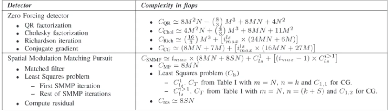
Fig. 1. Empirical CDF and limit condition number for (a)N=128,|L| =8 and (b)N=128,|L| =32.
converges almost surely in the asymptotic limit of transmit and receive antennas to [45, Theorem 7.3]
(HT)−−−−→ N,|L|→∞ 1+√1/β (|L|) 1−√1/β (|L|)= 11+−√√β (|L|) β (|L|) . (27) Equation (27) provides a useful approximation to determine the maximum condition number of a Rayleigh channel with a high number of receive antennas [4]. This can be seen in Fig. 1, where the CDF of the condition number of a Rayleigh fading channel matrix with N=128 receive antennas is depicted. The number of columns is|L| =8 and|L| =32 for Fig. 1(a) and (b) respectively. From the results of this figure it can be concluded that the condition number of the channel matrix is below the bound shown in (27) with a high probability. To conclude the argument, (27) is substituted into (23). In spite of being valid in a high number of cases, the probability of requiring a higher number of iterations for certain badly conditioned channels cannot be quantified with the above approximation. For this reason, in the following we resort to the analysis of the CDF of the modified condition number
F(ξ)=P(≤ξ)withξ ≥1 developed in [44]. To do so, we first defineσ [σ1, σ2, . . . , σk]as the ordered eigenvalues of
the Wishart matrix defined in (20) so that 0< σ1≤. . .≤σk.
Moreover, let V(σ) be the Vandermonde matrix with m,n-th entryvm,n=σnm−1[30, Section 4.6]. The CDF of the modified
condition numberof an uncorrelated central Wishart matrix is given by [44, Equation (9)] F(ξ)= k m=1 (s−m)! k n=1 (t−n)! −1 k l=1 ∞ 0 |ϒ|dσk. (28)
Here,|ϒ|denotes the determinant of the matrixϒ, whosem, n-th entryυm,nis defined as υm,n= ⎧ ⎨ ⎩ γ (t−k+m+n−1, ξσk) −γ (t−k+m+n−1, σk) , m=l v2 m,nσ t−k l e−σl , m=l (29)
where γ (a,b)is the lower incomplete gamma function given byγ (a,b)=0be−tta−1dt. Equations (28) and (29) allows us to
estimate the CDF of the condition number of a communication channel, which in turn is necessary to determine the number of LS iterations as shown in the following. Using the above results, the following theorem can be stated:
Theorem 1: The probability that a given number of LS iterationsilsmaxsuffices to achieve a relative error reduction of
εin the LS CG algorithm is given by
P ils≤ilsmax =F ⎛ ⎜ ⎝ ⎡ ⎣2·ilsmax log 2 ε ⎤ ⎦ 2⎞ ⎟ ⎠. (30)
Proof: The first step to derive (30) is to note that the definition of the condition number used in [44] varies with respect to the one employed in [41], [45]. Attending to their relationship, which is shown in (19), the CDF of the standard condition numbercan be expressed as
F(θ)=P(≤θ)=F(θ2). (31) In plain words,F(θ2) gives the probability that for a given constantθ, the condition number of the LS matrix is below that value. The solution of the above expression can be immediately obtained via numerical integration [44]. Once the CDF of the standard condition number has been characterized, the number of iterations of the CG algorithm in the considered scheme can be determined. Particularly, by using (23) the probability that a given number of LS iterationsilsmax achieves a relative error reduction ofεcan be expressed as
P ils≤ilsmax =P ⎛ ⎝≤ 2·ilsmax log 2 ε ⎞ ⎠. (32)
The proof is completed by substituting (32) into (31). The result of Theorem 1 can be used to show the trade-off between accuracy and complexity of the CG when the number of LS iterations is varied. In other words, (30) characterizes the impact of varying the number of iterations of the CG algorithm in the performance of the ZF and greedy CS detectors.
B. Convergence Rate and Error Analysis of CS-Based Detection in Large-Scale MIMO
The evolution of the error at thei-th iteration between the original signal and the sparse approximation is studied in [38] provided that the assumptionδ4S<0.1 on the restricted
isometry constant is satisfied. In this section we derive a more intuitive metric to characterize the error reduction based on the number of antennas used for signal transmission and recep-tion. In particular, we apply the results on the maximum and minimum singular values of a random Gaussian matrix to the analysis developed in [38] to derive the following bound.
Theorem 2: The Euclidean norm of the error between the sparse signal at thei-th iteration of the generic and SMMP CS algorithms and the transmitted signal is upper bounded by
x− ˜xi2≤c1(N,S)x− ˜xi−12+c2(N,S)w2. (33)
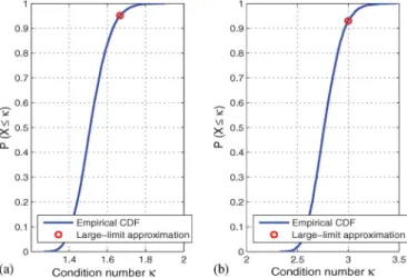
Fig. 2. Theoretical and empirical evolution of the maximum Euclidean norm of the error vs. number of iterations forN=128,K=16,nt=4,na=1, imax=4,k=2K, SNR=4 dB, 4-QAM and 105channel realizations.
Here, c1(N,S) andc2(N,S)depend on the number of active antennas for transmission and reception and are given by
c1= ⎛ ⎜ ⎝2+ T4S 2+4√β(4S) β(4S) T3S 1−√β(1 3S) 2 ⎞ ⎟ ⎠ × T4S T2S 1+2√β(4S) β(4S) +1+2√β(2S) β(2S) 1−√ 1 β(2S) 2 , (34) c2= ⎛ ⎜ ⎝2+ T4S 2+4√β(4S) β(4S) T3S 1−√β(1 3S) 2 ⎞ ⎟ ⎠ ⎛ ⎜ ⎝ 2+√β(2 2S) √ T2S 1−√β(1 2S) 2 ⎞ ⎟ ⎠ +√ 2 T3S− √ T3S √β( 3S) , (35) whereTCmax(N,C),C∈R+.
Proof: The proof is shown in Appendix A. Note that, as opposed to [38], (40) and (41) show the direct relationship between the norm bounds and the dimensions of the measurement matrix. In other words, the RIP hypothesis is not longer necessary thanks to the use of the random matrix theory results. The bound derived in (33) allows characterizing the error reduction per iteration as a function of the number of receive antennas. In other words, the convergence speed and performance of the algorithm is upper bounded by (33) as a smaller value of thec1(N,S)will allow obtaining a faster convergence whereasc2(N,S)characterizes the error floor. This is shown in Fig. 2, where the maximum empirical Euclidean norm of the error for the proposed algorithms is obtained over 105 channel realizations and compared with the analyt-ical bound. The theoretanalyt-ical result is obtained by using (33) with a number of receive antennas that guarantees algorithmic convergence [38]. In this figure, it can be seen that the use of a theoretical large-scale approximation allows us to upper
bound the evolution of the empirical maximum2norm of the error for a practical number of iterations. Moreover, Fig. 2 also depicts the faster convergence and reduction in the maximum Euclidean norm of the error offered by the SMMP algorithm w.r.t. the straightforward CS approach.
VII. ENERGYEFFICIENCY
The study of the EE becomes especially important in the uplink of multi-user scenarios due to the necessity of finding energy-efficient schemes that allow increasing the battery life-time [1]. In this section, we define the EE model that will be used hereafter to characterize the EE improvements offered by the proposed technique in the MAC when compared to other detection schemes. Towards this end, we express the EE as the rate per milliwatt of total consumed power by using the metric [26], [46]–[52]
= Se "K
u=1Pu
subject to BER≤BERobj. (36)
Here, BERobj is the objective average BER,Se refers to the
spectral efficiency in bits per channel use (bpcu), andPuis the
total power consumption of theu-th MS in milliwatts required to achieve a given BERobj. The total power consumption per
MS can be expressed as [47] Pu=PCu+PTu= [Pψ+P] + ⎡ ⎣ ⎛ ⎝nt j=1 pu,j ⎞ ⎠·ζ ⎤ ⎦. (37)
In the previous expression, PCu=Pψ+P denotes the total
circuit power consumption excluding the power amplifier (PA) and it is divided into two components: Pψ that represents the circuit power consumption that depends on the number of active antennas, and P that corresponds to the static power consumption and it is fixed to a reference value of 5 mW per MS [47]. In particular,Pψ comprises the additional power consumption required to activate the circuitry of the RF chains and the digital signal processors for transmission. Moreover,
PTu= "nt
j=1pu,j·ζrefers to the power consumption of the PAs and it depends on the factorζ = νη and the power of the signal that is required to be transmitted by each of the antennaspu,j.
In the last expression, the factorνis the modulation-dependent peak to average power ratio (PAPR) andηcorresponds to the PA efficiency [46]. Based on the above, the global EE can be expressed as = Se "K u=1 # [Pψ+P] +"nt j=1νη ·pu,j $,
subject to BER≤BERobj. (38)
For the simulations of this work, the efficiency factor corre-sponds to the one of a class-A amplifier, η=0.35, which is commonly used in this setting due to the linearity required to transmit QAM signals [46].
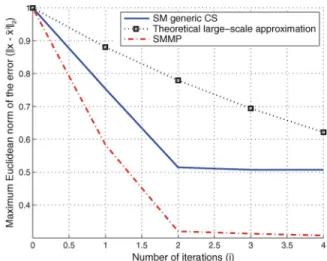
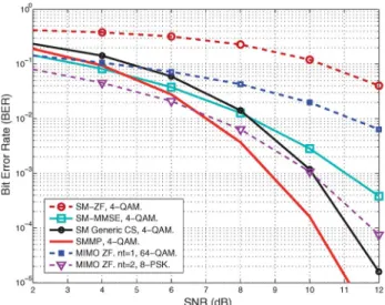
Fig. 3. BER vs. SNR forN=128,K=S=16,nt=4,na=1,imax=2, k=KandSe=64 bpcu.
VIII. SIMULATIONRESULTS
Monte Carlo simulations have been performed to charac-terize the performance and complexity improvements of the proposed technique. To maintain the coherence with the SM literature, we compare conventional massive MIMO systems and SM systems with the same spectral efficiency. The per-formance and energy efficiency results of spatial multiplexing systems with the same number of transmit antennas have not been represented in these figures to avoid congestion and because they exhibit a worse behavior when compared to the spatial multiplexing systems considered here. In the following, SM-ZF and SM-MMSE refer to the linear ZF and MMSE detectors introduced in Section II-C, SM Generic CS denotes the CoSaMP algorithm without the improvement described in Section III, and the techniques with MIMO on their description correspond to those of a conventional MIMO scenario without SM. For reasons of brevity, in this section we selectk=Sfor the generic and SMMP CS algorithms. Note that this decision entails a minimization of the computational complexity for the CS-based algorithms following the results of Table II. Additionally, we also consider the MPD algorithm in spite of its increased computational complexity [23]. The performance results, unless stated otherwise, have been obtained with an exact solution of the LS problem via Cholesky decomposition for clarity.
Fig. 3 characterizes the performance of the above-mentioned detectors in a scenario withN=128,K=16,nt=4,na=1
corresponding to the single active antenna SM, and a resulting spectral efficiency of Se=64 bpcu. The results of this
fig-ure have been obtained withimax=2 iterations of Algorithm
1, which ensures a reduced complexity when compared to the algorithms developed in [23]. Note that an error floor is expected due to the non-feasible solutions produced by the generic CS algorithm. This, however, cannot be appreciated in these results since the high number of antennas considered at the BS moves the error floor to very low BER values [18]. Fig. 3 shows that the proposed algorithm is able to reduce the required transmission power by more than 4 dB w.r.t.
Fig. 4. BER vs. SNR forN=128,K=16,nt=7,na=2,imax=3,k= S=2KandSe=96 bpcu.
conventional MIMO with nt=1 and 16-QAM to achieve a
target BER of 10−4. Moreover, it is portrayed that SMMP approaches the performance of the more complex MPD and outperforms the SM-ZF detector. This is because the proposed strategy is able to iteratively identify the active antenna indices and then perform a selective channel inversion with a matrix of reduced dimensions. Instead, the performance of conventional MIMO with two active antennas per user approaches the per-formance of SMMP. However, we remark that in this case the power consumption and complexity of the MSs is increased due to the additional RF chains implemented.
Fig. 4 shows the performance of the considered detectors in a scenario withN=128, K=16,nt=7, generalized SM
withna=2 active antennas per user, and a resulting spectral
efficiency of Se=96 bpcu. The results of this figure show
that generalized SM systems with SMMP detection are capable of improving the performance of conventional MIMO systems employing the same number of RF chains (‘MIMO-ZF.nt =
1’). The use of SMMP also allows outperforming conventional MIMO systems with a pair of RF chains (‘MIMO-ZF.nt=2’)
for the range of practical BERs. Moreover, it can be seen that the SMMP algorithm clearly improves the performance of other linear detectors such as the SM-MMSE detector. In the following we focus our attention on single active antenna SM for reasons of brevity, although it is clear that the resultant conclusions also extend to generalized SM transmission.
The number of users is increased fromK=16 of Fig. 3 to
K=32 in Fig. 5, which shows a scenario especially favorable for the proposed technique. Fig. 5 shows that the proposed strategy is able to provide an enhancement of up to three orders of magnitude in the BER at high SNR values w.r.t. conventional large-scale MIMO, and both ZF and MMSE detectors in SM. The performance improvement offered by SM when compared to conventional MIMO transmission is coherent with the behav-ior described in [20], [53]. The effect of acquiring inaccurate channel state information (CSI) on the performance is also shown in Fig. 5(b). The imperfect CSI is modeled following
%
H=√1−τ2H+τB, whereτ ∈ [0,1]regulates CSI quality
Fig. 5. BER vs. SNR forN=128,K=S=32,nt=4,na=1,imax=3, k=KandSe=128 bpcu with (a) perfect and (b) imperfect CSI(τ=0.25).
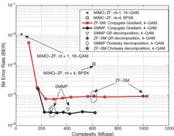
Fig. 6. BER vs. complexity for N=128, K=S=16, nt=4, na=1,
SNR=6 dB,Se=64 bpcu,imax=2,k=Kwith different LS methods.
and B∈CN×M ∼CN(0,IN⊗IM) characterizes the channel
estimation error [54]. The results of this figure for τ =0.25 highlight the robustness of SMMP when compared to tradi-tional CS-based detection, which makes it the best alternative in terms of performance under imperfect CSI.
Fig. 6 shows the trade-off between performance and com-plexity in real flops for a MAC withN=128,K=16,na=1, Se=64 bpcu,imax=2,k=Kand SNR=6 dB. The number
of antennas per user isnt=4 when SM is used, whereas it is nt=1 andnt =4 for conventional MIMO. Note that the
com-plexity and performance of the CG algorithm varies depend-ing on the number of iterations as explained in Section V-A. From the results of this figure it can be concluded that the SMMP approach offers the best performance with a restrained complexity. When compared to large-scale MIMO systems with the same spectral efficiency and alike number of RF chains (‘MIMO-ZF,nt=1’), the use of SM increases the complexity
due to the higher number of antennas at the MSs, but in turn offers a performance improvement of more than two orders of
Fig. 7. BER vs. complexity forN=128,K=S=8,nt=4,na=1, SNR=
2 dB,Se=32 bpcu,imax=2,k=Kwith different LS methods.
magnitude. This improvement is not as significant with respect to the spatial multiplexing system with the same number of antennas (‘MIMO-ZF,nt =4’), where instead the complexity
is dramatically reduced. Fig. 6 also shows the complexity improvements that can be obtained when the iterative CG algo-rithm termed ‘ZF-SM. Conjugate Gradient’ considered in this paper is used to solve the LS problems against traditional direct methods such as ‘ZF-SM. QR decomposition’ and ‘ZF-SM. Cholesky decomposition’ in Fig. 6. The number of iterations and, inherently, the complexity can be adjusted depending on the BER required at the BS. This leads us to conclude that the use of the CS-based detection is especially convenient in fast fading scenarios with a reduced channel coherence period. This is because whereas CS-based detection methods perform the same computations in every channel use, the linear detectors solved with direct methods focus the intensive computations at the beginning of the coherence period and reduce the complex-ity afterwards [2].
A similar conclusion can be obtained from the results of Fig. 7, where we focus on controlling the attainable perfor-mance by varying the number of LS iterations in the CG algorithm. We also note that, as opposed to the conclusions achieved in [18], [38], the iterative LS algorithm accounts for 60% of the global detection complexity, hence justifying the need of an accurate complexity characterization. Overall, it can be concluded that the proposed strategy offers significant performance and complexity improvements with respect to con-ventional detection schemes in systems with the same number of antennas.
Regarding the EE of the CS-based detection, Fig. 8 shows this metric for a MAC with N=128 and a varying number of users. The transmission power is varied depending on the number of users so that BERobj=10−3 in (36). The circuit
power consumption depending on the number of active anten-nas is set to a realistic value ofPψ =20 mW [46], and the noise variance is fixed toσ2=0.01. We note that the PAPR factor of the single-antenna users is increased w.r.t. SM due to the use of a higher modulation orderQ. From the results of this figure it can be concluded that the use of SM allows to significantly
Fig. 8. EE vs. number of usersKto achieve BER=10−3.N=128,nt=4, na=1.Pψ=20 mW.
Fig. 9. EE vs. number of usersKto achieve BER=10−3.N=128,nt=4, na=1.Pψ=10 mW.
increase the EE of the conventional large-scale MIMO for low and intermediate system loading factors. This improvement due to the reduced circuit power consumption and PAPR was already noticed in [55] for the downlink of small-scale P2P systems. Moreover, the proposed technique outperforms the rest of conventional detectors, hence constituting an energy-efficient alternative in the MAC.
Fig. 8 also shows that, in spite of the transmission energy savings that can be obtained whennt =2 and 4-QAM are used
in MIMO systems, the increased circuit power consumption caused by the higher number of RF chains penalizes the EE. To show this effect, in Fig. 9 we reduce the power consumed by the RF chainsPψ to half, i.e.,Pψ =10 mW. By doing so, now it can be seen that the use of a MIMO system withnt=2
outperforms the option of having single-antenna devices. Still, the EE of the SM alternatives is significantly higher than the one of MIMO strategies for a low and intermediate number of users due to the reduced transmission power required to compensate the inter-user interference.
IX. CONCLUSION
In this paper, a low-complexity detection algorithm for SM has been presented. The proposed strategy is based upon CS by incorporating the additional structure and sparsity of the trans-mitted signals in the MAC. Our complexity and performance analyses show that the benefits of the proposed are maximized when a high number of receive antennas at the BS are used due to its faster convergence and improved performance. Overall, the results derived in this paper confirm that the CS-based detection for SM constitutes a low-complexity alternative to increase the EE in the MAC. Possible future work can be carried out in the analytic characterization of the bit error rate performance of the proposed scheme in the large-scale regime.
APPENDIXA PROOF OFTHEOREM2
The proof of Theorem 2 commences by recalling the re-sults regarding the maximum and minimum singular values of Wishart matrices with large dimensions [4]. LetWbe the Wishart matrix defined in (20) with the entries of the matrix HL∈CN×|L| satisfying hm,n∼CN(0,1). For these
expres-sions, no assumptions on the definition and cardinality of L andR are adopted. For large N and |L|, the maximum and minimum eigenvalues ofWconverge to
σmin(W) −→ N,|L|→∞T|L|× 1−√ 1 β (|L|) 2 σmax(W) −→ N,|L|→∞T|L|× 1+√ 1 β (|L|) 2 (39) where β(V) was defined in (26) and TCmax(N,C),C∈ R+. Based on the above expressions, we can redefine some relationships that will be useful in the sequel
HH Ly2≤ T|L|× 1+√ 1 β (|L|) y2, H†Ly 2≤ ⎛ ⎝ 1 T|L|× 1−√ 1 β(|L|) ⎞ ⎠y2, HHLHLx2T|L|× 1±√ 1 β (|L|) 2 x2, HHLHL−1x 2 ⎛ ⎝ 1 T|L|× 1±√ 1 β(|L|) ⎞ ⎠ 2 x2. (40)
Note that the last two inequalities can determine upper and lower bounds [38]. Moreover, the following relationship is also satisfied
HH
RHL≤ β(TBB)+√2β(TB
B), (41)
where the set G with cardinality B is given by GR∪L. As the derivation of the previous expression is based upon the ideas developed in [38], but considering instead that the spectral
norm ofHHRHL is always smaller than the one ofHHGHG−T
and that the functionβ :Z+→R+, here we avoid a detailed description for brevity.
The objective of the proof is to establish an upper bound on the2norm of the error between the transmitted signal and the approximation obtained by the generic CS algorithm at thei-th iteration [38], i.e.,
x− ˜xi2≤Rmax, (42)
whereRmaxis the upper bound to be derived andx˜iis the
esti-mated signal at thei-th iteration. The upper bound is obtained by following the arguments developed in [38] and applying the results obtained in (40) and (41) where convenient. To preserve the coherence with [38], in the following it has been assumed that|T| ≤3Sor, in other words,|| =2Sentries are selected at the output of the MF per iteration.
To derive the desired result, first note that the difference between the S-sparse transmitted signal x and the output of the LS problembis bounded when selecting the bestS-sparse approximationx˜i[38]. Formally,
x− ˜xi2≤ x−b2+ b− ˜xi2≤2x−b2, (43) where the basic norm propertya+z ≤ a + zhas been applied. With the purpose of deriving an upper bound to the right-hand side of (43), we first expressx−b2as
x−b2≤ x|TC2+ x|T −b|T2, (44)
where the inequality holds because b is supported on T fol-lowing (18). We now focus on deriving an upper bound for
x|T −b|T2, which is given by x|T −b|T2 (a) =x|T −H†T(Hx|T +Hx|TC+w) 2 (b) ≤ HHTHT−1HHTHx|TC 2+ H†Tw 2 (c) ≤ ⎛ ⎜ ⎝ T4S β(4S) + 2T4S √β( 4S) T3S 1−√β(1 3S) 2 ⎞ ⎟ ⎠x|TC2+ w2 √ T3S− √ T3S √ β(3S) . (45) In the above expressions, (=a) holds by definition (18), and(≤b) follows from the definition of the pseudoinverse matrix and by noting thatH†THx|T =x|T. Moreover,(≤c)is obtained by using the relationships derived in (40) and (41) along with the fact that, by definition,|T| ≤3SandxisS-sparse. Substituting the last inequality of (45) into (44) we obtain the desired upper bound x−b2≤ ⎛ ⎜ ⎝1+ T4S β(4S)+ 2T4S √β( 4S) T3S 1−√β(1 3S) 2 ⎞ ⎟ ⎠x|TC2+ w2 √ T3S− √ T3S √β( 3S) . (46)