Group Lasso for generalized linear models in high
dimension
M´
elanie Blaz`
ere, Jean-Michel Loubes, Fabrice Gamboa
To cite this version:
M´
elanie Blaz`
ere, Jean-Michel Loubes, Fabrice Gamboa. Group Lasso for generalized linear
models in high dimension. 2014.
<
hal-00850689v3
>
HAL Id: hal-00850689
https://hal.archives-ouvertes.fr/hal-00850689v3
Submitted on 22 Jan 2014
HAL
is a multi-disciplinary open access
archive for the deposit and dissemination of
sci-entific research documents, whether they are
pub-lished or not.
The documents may come from
teaching and research institutions in France or
abroad, or from public or private research centers.
L’archive ouverte pluridisciplinaire
HAL
, est
destin´
ee au d´
epˆ
ot et `
a la diffusion de documents
scientifiques de niveau recherche, publi´
es ou non,
´
emanant des ´
etablissements d’enseignement et de
recherche fran¸cais ou ´
etrangers, des laboratoires
publics ou priv´
es.
Oracle inequalities for a Group Lasso procedure applied to
generalized linear models in high dimension
M´
elanie Blaz`
ere, Jean-Michel Loubes and Fabrice Gamboa
Abstract
We present a Group Lasso procedure for generalized linear models (GLMs) and we study the properties of this estimator applied to sparse high-dimensional GLMs. Under general conditions on the covariates and on the joint distribution of the pair covariates, we provide oracle inequalities promoting group sparsity of the covariables. We get convergence rates for the prediction and estimation error and we show the ability of this estimator to recover good sparse approximation of the true model. Then we extend this procedure to the case of an Elastic net penalty. At last we apply these results to the so-called Poisson regression model (the output is modeled as a Poisson process whose intensity relies on a linear combination of the covariables). The Group Lasso method enables to select few groups of meaningful variables among the set of inputs.
Keywords: Generalized linear model, high dimension, sparse model, groups of variables, Group Lasso, oracle inequalities.
1
Introduction
Handling high dimensional data is nowadays required for many practical applications ranging from astronomy, economics, industrial problems to biomedicine. Being able to extract information from these large data sets has been at the heart of statistical studies over the last decades and many papers have extensively studied this setting in a lot of fields ranging from statistical inference to machine learning. We refer for instance to references therein.
For high-dimensional data, classical methods based on a direct minimization of the empirical risk can lead to over fitting. Actually adding a complexity penalty enables to avoid it by selecting fewer coefficients. Using anℓ0 penalty leads to sparse solutions but the usely non-convex
mini-mization problem turns out to be extremely difficult to handle when the number of parameters becomes large. Hence the ℓ1 type penalty has been introduced to overcome this issue. On the
one hand this penalty achieves sparsity of an estimated parameter vector and on the other hand it requires only convex optimization type calculations which are computationally feasible even for high dimensional data. The use of aℓ1 type penalty, first proposed in [25] by Tibshirani, is now
a well established procedure which has been studied in a large variety of models. We refer for example to [2], [5], [26], [8], [24], [32] and [4].
Group sparsity can be promoted by imposing a ℓ2 penalty to individual groups of variables
and then aℓ1 penalty to the resulting block norms. Yuan and Lin [31] proposed an extension of
the Lasso in the case of linear regression and presented an algorithm when the model matrices in each group are orthonormal. This extension, called the Group Lasso, encourages blocks sparsity. Wei and Huang [29] studied the properties of the Group Lasso for linear regression, Nardi and Rinaldo [18] established asymptotic properties and Lounici, Pontil, van de Geer and Tsybakov [14] stated oracle inequalities in linear Gaussian noise under group sparsity. Meir, van de Geer and B¨uhlmann [17] considered the Group Lasso in the case of logistic regression and Zhang and Huang [32] studied the benefit of group sparsity. Another important reference is the work of Negahban, Ravikumar, Wainwright and Yu [20]. In this last paper a unified framework for the study of rates of convergence in high dimensional setting is provided under two key assumptions (restricted strong convexity and decomposability). This work and these two assumptions will be discussed in more details in Section3.
In this paper we focus on the Group Lasso penalty to select and estimate parameters in the generalized linear model. One of the application is the Poisson regression model. More precisely, we consider the generalized linear model introduced by McCullagh and Nelder [16]. Let F be a distribution on R and let (X, Y) be a pair of random variables with X ∈ Rp and Y ∈ R. The
conditional law of Y|X = x is modeled by a distribution from the exponential family and the canonical parameter is the linear predictor. Thus the conditional distribution of the observations givenX =xisP(Y|β∗, x) = exp(yβ∗Tx
−ψ(β∗Tx)), whereβ∗TxsatisfiesRexp(yβ∗Tx)F(dy)<∞ and ψ is the normalized function. Notice that E(Y|X) a.s= ψ′(β∗TX) in other words β∗TX a.s=
h(E(Y|X)) where h=ψ′−1 is the so-called link function. Some common examples of generalized
linear models are the Poisson regression for count data, logistic and probit regression for binary data or multinomial regression for categorical data. The quantities of interest that we would like to estimate are the component (β∗
j)16j6p of β∗ and for a given x we may also wish to predict
the responseY|X =x. A natural field of applications for such models is given by genomics and Poisson regression type models. In particular thousands of variables such as expressions of genes and bacterias can be measured for each animal (mices) in a (pre-)clinical study thanks to the developpement of micro arrays (see, for example, [3] and [7] ). A typical goal is to classify their health status, e.g. healthy or diseased, based on their bio-molecular profile, i.e. the thousands of bio-molecular variables measured for each individual (see for instance [9], [22] and [21]).
The paper falls into the following parts. In Section2we describe the model and the Group Lasso estimator for generalized linear models. In Section 3 we present the main results on coefficients estimation and prediction error and in Section 4 we consider the model in the particular case of a Poisson regression. We also study here the general model in the case of a mixture of anℓ1 and
ℓ2 penalty. The Group Lasso estimator is then used on simulated data sets in Section 5 and its
performances are compared to those of the Lasso estimator. The Appendix is devoted to the proof of the main theorems.
2
Sparse Variable selection for generalized linear models
2.1
The model
The Exponential family on the real line is a unified family of distributions parametrized by a one dimensional parameter and is widely used for practical modelling. LetF be a probability distribution onRnot concentrated on a point and
Θ := θ∈R: Z exp(θx)F(dx)<∞ . Define M(θ) := Z exp(θx)F(dx) (θ∈Θ) and ψ(θ) := log(M(θ)) (θ∈Θ).
LetP(y;θ) = exp(θy−ψ(θ)) withθ∈Θ. The densities of probability (related to a mesure adapted to the continuous or discrete case){P(.;θ) :θ∈Θ}is called the exponential family. Θ is the natural parameter space andθis called the canonical parameter. The exponential family includes most of the commonly used distributions like normal, gamma, poisson or binomial distributions [16].
We consider a pair of random variables (X, Y) where Y ∈ R and X ∈ Rp such that the
conditional distribution Y|X =xis P(Y|β∗, x) = exp(yβ∗Tx
−ψ(β∗Tx)), with β∗Tx∈ Θ. Our aim is to estimate the components (β∗
j)16j6p of β∗ in order to predict the response Y|X = x
conditionally on a given value ofx. We assume that
• (H.1): the variableX is almost surely bounded by a constantL i.e. there exists a constant
L >0 such thatkX k∞6La.s.
and we consider
Λ =β ∈Rp: ∀x∈[−L, L]p, βTx∈Θ .
Let (X1, Y1), ...,(Xn, Yn) be i.i.d copies of (X, Y) where Xi = (Xi,1, ..., Xi,p)T fori= 1, ..., n. We
consider the case of high-dimensional regression i.e p≫ n. The log-likelihood for a generalized linear model is given by
L(β) = n X i=1 YiβTXi−ψ(βTXi).
We denote the generalized linear model loss function by
l(β) =:l(β;x, y) =:−yfβ(x) +ψ(fβ(x)), (1)
wherefβ(x) :=βTx. Notice that this function is convex inβ (asψis convex). The associated risk
is defined byPl(β) =:El(β;Y, X) and the empirical risk byPnl(β) where Pnl(β) := 1 n n X i=1 −YiβTXi+ψ(βTXi) . Obviously β∗= argmin β∈Λ Pl(β).
2.2
Group Lasso for generalized linear model
Assume thatX is structured intoGn groups each of sizedg forg∈ {1, ..., Gn}. Fori= 1, ..., n
we set Xi= (Xi1, ..., X g i, ..., X Gn i )T where Xig= (Xi,g1, ..., Xi,dgg )T
and PGng=1dg = p. This decomposition is often natural in biology and micro arrays data when
the covariates are genes expresssion (see for instance [23] and [30]). We allow the number of groups to increase with the sample size n, so we can consider the case where Gn ≫ n. Define
dmax := max
g∈{1,...,Gn}dg and dmin:=g∈{1min,...,Gn}dg. Forβ ∈
Rp we denote byβg the sub-vector ofβ
whose indexes correspond to the index set of thegthgroup ofX.
Let us consider the Group Lasso estimator which achieves group sparsity and is obtained as the solution of the convex optimization problem
ˆ βn = argmin β∈Λ ( Pnl(β) + Gn X g=1 s(dg)kβgk2 )
wherern is the tuning parameter.
Here k.k2 refers to the Euclidian norm and s is a given function. An increase in rn leads
to a diminution of theβg to zero, this means that some blocks become simultaneously zero and
groups of predictors drop out of the model. Typically we chooses(dg) :=pdg to penalize more
heavily groups of large size. Notice that if all the groups are of size one then we recover the Lasso estimator. The Group Lasso achieves variables selection and estimation simultaneously as the Lasso does. The penalty function is the sum of theℓ2 norm of the groups of variables. Thus
the Group Lasso estimator acts like the Lasso at the group level [18], [14], [31]. Actually the objective function above is the sum of a particular loss function (which is convex and based on the exponential family) with a weighted regularizer. This type of convex optimization problem is referred as a regularized M-estimator in the paper of Negahban et al. [20]. We can also notice that the penalty norm satisfies the decomposability condition defined in this last paper.
We study estimation and prediction properties of the Group Lasso in high dimensional settings when the number of groups exceeds the sample size i.e. Gn ≫n. Define H∗={g:β∗g 6= 0} the
Such a set characterizes the sparsity of the model. In the followingH∗c denotes the index set of the groups which are not inH∗. We can notice thatH∗ andm∗ depend onnbut for simplicity we
do not specify this dependency. In general, it will be hopeless to estimate all unknown parameters from data except if we make the assumption that the true parameter is group sparse. In this paper we consider that β∗ is partitioned into a number of groups, in correspondance with the
partition ofX, only few of which are relevant. The index of group sparsity m∗ will be discussed
more deeply after Theorem3.7. We also assume (H.3): there exists a constant B >0 such that
PGn g=1
p
dgkβ∗gk26B.
3
Main Results
3.1
Bounds for estimation and prediction error
Under some assumptions on the value of the parameterrn and on the covariance matrix ofX
we are going to show the ability of this estimator to recover good sparse approximation of the true model. To prove oracle inequalities for the Group Lasso applied to generalized linear model we need to state concentration inequalities for the empirical process Pn(l(β)) for β ∈ Λ. This step
is essential to compute an appropriate lower bound for the regularization parameter that ensures good statistical properties of the estimator with high probability. Notice that this step requires a boundedness assumption on the (Xi,j) (cf. proof of Proposition3.1).
To state concentration inequalities we first break down the empirical process into a linear part and a part which depends on the normalized parameterψ
(Pn−P) (l(β)) = (Pn−P) (ll(β)) + (Pn−P) (lψ(β))
wherell(β) :=ll(β, x, y) =−yβTxandlψ(β) :=lψ(β, x) =ψ(βTx).Define
A= Gn \ g=1 {Lg6rn/2} where Lg:= 1 p dgn n X i=1 (YiXig−E(Y X g)) 2
for allg∈ {1, ..., Gn}and
B= sup β:PGng=1 √ dgkβg−β∗gk 26M |νn(β, β∗)|6 rn 2 where νn(β, β∗) := (Pn−P) (lψ(β∗)−lψ(β)) PGn g=1 p dgkβg−β∗gk2+εn
withM = 8B+εn andεn = n1. We assume thatGn andnare such that log(2nGn) 61. The next
proposition shows that the event A ∩ B occurs with high probability for some suitable values of the tuning parameter.
Proposition 3.1. Let rn>AKL CL,B∨ max {|x|6Lκn}∩Θ|ψ ′ (x)|) r 2 log(2Gn) n
whereK is a universal constant,A >√2,κn:= 17B+2n andCL,B is defined in Lemma3.2. We
have
P(A ∩ B)>1−(C+ 2dmax)(2Gn)−A
2
/2.
The proof rests on concentration inequalities and is detailled in the appendix. Indeed infering a bound for the probability of the eventsAandBis equivalent to prove concentration inequalities for the linear and non linear part of the empirical process. A concentration inequality for the linear part is derived from Bernstein inequality once the following lemma has been proved. This lemma provides moment bounds forY.
Lemma 3.2. Let(X, Y)a pair of random variables whose conditional distribution isP(Y;β∗|X =
x) = exp(yβ∗Tx−ψ(β∗Tx)) and assume assumptions (H.1-3) are fulfilled. For all k ∈N∗ there
exists a constantCL,B (which depends only on LandB) such thatE(|Y|k)6k!(CL,B)k.
The boundedness assumption on the components ofX is required to prove this lemma. Then, for the non linear part of the empirical process, we use again this assumption to show that we can restrict the study ofψ to a suitable compact set. Sinceψ is lipchitzian on this compact set, concentration results for lipchitzian loss functions (see [12]) allow to bound the probability of the eventB.
Thus, on the event A which occurs with high probability (see Proposition 3.1), we have an upper bound for the linear part of the empirical process (Pn−P)ll(β∗)−l
l( ˆβn)
.
Proposition 3.3. On the eventA
(Pn−P)ll(β∗)−ll( ˆβn)6rn 2 Gn X g=1 p dgkβˆng−β ∗g k2. Proof. We have (Pn−P)ll(β∗)−ll( ˆβn) = Gn X g=1 ( ˆβng−β ∗g )T " 1 n n X i=1 YiXig−E(Y X g) # 6 Gn X g=1 p dgkβˆgn−β ∗g k2 1 p dgn n X i=1 (YiXig−E(Y X g)) 2 .
The last bound is obtained by using Cauchy-Schwarz inequality. Then on the eventAthe propo-sition follows.
Therefore the difference between the linear part of the empirical process and its expectation is bounded from above by the tuning parameter multiplied by the norm (associated to the Group Lasso penalty) of the difference between the estimated parameter and the true parameterβ∗. We
can state a similar result for the non linear part of the empirical process, the key of the proof is based on the fact that the estimator ˆβn is in a neighborhood of the target parameterβ∗ on the
eventATB.
Lemma 3.4. On the event ATB we have PGng=1pdgkβˆng −β∗gk2 6 M, where we recall that
M = 8B+εn andεn= 1n.
Then the next proposition provides an upper bound for (Pn−P)lψ(β∗)−l ψ( ˆβn)
and is directly involved by the definition ofB and Lemma3.4.
Proposition 3.5. On the eventA ∩ B
(Pn−P)lψ(β∗)−lψ( ˆβn) 6rn 2 Gn X g=1 p dgkβˆng−β∗ g k2+εn ! .
Once concentration of the loss function around its mean is stated, we have to ensure that the loss function is not too flat in such a way that if the loss difference l( ˆβn)−l(β∗) converges to
zero then ˆβn converges toβ∗. In this paper such a property holds assuming that the covariance
matrix satisfies a Group Stabil condition (see condition below). This condition is closely related to the one of Negahban et al. [20] called Restricted Strong Convexity property. Notice that in our analysis the boundedness of the covariates is required to prove such a property. In fact, thanks to the boundedness of the covariates, we first bound from below the mean deviation of the loss function by a quadratic function (see PropositionA.1in Appendix A). This first step enables to relate the deviation in the loss to the deviation of the estimated parameter from the true one. Then the Group Stabil condition implies that the loss function satisfies a local strong convexity property. This has been characterized as a common step for convergence of M-estimator (see [20]). Notice that the boundedness assumption on the components ofX is not required to obtain a kind of strong convexity. For example, as stated by Negahban et al., if the covariates have sub-gaussian tails and if the covariance matrix is positive definite then the loss function satisfies a form of restricted strong convexity property with high probability. However, as noticed above the boundedness assumption is necessary to establish Proposition3.1.
Therefore the key condition to derive oracle inequalities rests on the correlation between the covariates i.e. on the behavior of the Gram matrix 1nPni=1XiXiT which is necessarily singular
when p > n. Meier, van de Geer and B¨uhlmann [17] proved that the group Lasso is consistent in the particular case of logistic regression and gave bounds for the prediction error under the assumption thatE(XXT) is non singular. In this paper we give sharp bounds for estimation and
prediction errors for generalized linear models using a weaker condition similar to the restricted eigenvalue condition (RE) of Bickel, Ritov and Tsybakov [2]. This condition is quite weaker than the one of Bunea, Tsybakov and Wegkamp [6]. In their article Bickel, Ritov and Tsybakov also give several sufficient conditions for RE (which are easier to check). Here we use a condition which is a group version of the Stabil Condition first introduced by Bunea [5] for logistic regression in the case of anℓ1 penalty. This condition is similar (within a constantε) to the condition used by
Lounici, Pontil, van de Geer and Tsybakov [14] to state oracle inequalities for linear regression. Forc0,ε >0, we define the restricted set as
S(c0, ε) = δ: X g∈H∗c p dgkδgk26c0 X g∈H∗ p dgkδgk2+ε .
On this set we assume that the covariance matrix satisfies the Group Stabil condition defined below. This condition ensures local stong convexity in a neighborhood ofβ∗.
Let Σ :=E(XXT) be thep×pcovariance matrix.
Definition : Group Stabil Condition
Letc0, ε >0 be given. Σ satisfies the Group Stabil conditionGS(c0, ε, k) if there exists 0< k <1
such that
δTΣδ>k X
g∈H∗
kδgk22−ε
for anyδ∈S(c0, ε).
Before going any further we have to define two norms that are used to control the estimation error. For allz∈Rp, let
kzkR:= Gn X g=1 p dgkzgk2 and kzk2,1:= Gn X g=1 kzgk2.
The normk.kR is called the regularizer norm.
We are now able to state the main result of this paper which provides meaningful bounds for the estimation and prediction error when the true model is sparse and log(Gn) is small as compared
Letγ∗:=P
g∈H∗dg. We recall thatκn:= 17B+
2
n.
Theorem 3.6. Assume conditionGS(3,21n, k) is fulfilled. Let
rn>AKL CL,B∨ max {|x|6Lκn}∩Θ|ψ ′ (x)|) r log(2Gn) n
whereA >√2,Kis a universal constant andCL,Bis defined in Lemma3.2. Then, with probability
at least1−(C+ 2dmax)(2Gn)−A 2
/2 (whereC is given in Proposition3.1), we have
kβˆn−β∗kR6 4 cnk rnγ∗+ 1 + 1 rn 1 2n, kβˆn−β∗k2,16 4 cnk√dmin rnγ∗+ 1 + 1 rn 1 2n√dmin and E ˆ βTnX−β ∗T X26 16 c2 nk rn2γ∗+ 2rn+ 1 2cnn . where cn:= min {|x|6L(9B+1 n)}∩Θ ( ψ′′(x) 2 ) .
Notice thatcn >0 since the measure associated to the distributionF is not concentrated on a
point.
These results are similar to those of Nardi and Rinaldino [18] who proved asymptotic properties of the Group Lasso estimator for linear models. We can notice that ifγ∗ =O(1) then the bound
on the estimation error is of the orderO
q
logGn n
and the Group Lasso estimator still remains consistent for the ℓ2,1-estimation error and for the ℓ2-prediction error under the Group Stabil
condition if the number of groups increases almost as fast asO(exp(n)). The term√logGn is the
price to pay for having a large number of factors and not knowing where are the non zero ones. Sincekβˆn−β∗k2≤ kβˆn−β∗k2,1, we also have
kβˆn−β∗k26 4 cnk√dmin rnγ∗+ 1 + 1 rn 1 2n√dmin .
However, a sharper bound for the l2-norm of the estimation error holds but under a stronger
assumption thanGS(3, 1 2n, k).
Theorem 3.7. Assume GS(2m∗,3, 1 2n, k
′
)i.e there exists 0< k′ <1 such that
δTΣδ>k′X g∈J kδgk2 2− 1 2n
for anyδ such thatPg∈Jc p
dgkδgk263Pg∈J p
dgkδgk2+21n andJ such that |J| ≤2m∗. Then
we have with probability at least1−(C+ 2dmax)(2Gn)−A
2/2 kβˆn−β∗k22610 dmax dmin ( 16 k′2 c2 n rn2γ∗+ 2rn+ 1 2k′c nn + 1 2k′n ) .
Proof. Let J∗ = H∗∪I and I is the set of indice corresponding to the m∗ largest values of p
dgkβˆng−β∗gk2 inH∗c. We can prove (see proof of Theorem 3.1 in [14] withλg=rn p dg ) that X g∈J∗c kβˆng−β ∗g k22≤9 dmax dmin X g∈J∗ kβˆng−β ∗g k22 (2)
and X g∈J∗c p dgkβˆng−β ∗g k263 X g∈J∗ p dgkβˆng−β ∗g k2+ 1 2n.
Therefore on one hand, using assumptionGS(2m∗,3, 1 2n, k ′ ), we deduce k′ X g∈J∗ kβˆng−β ∗g k22≤E ˆ βTnX−β ∗T X2+ 1 2n (3)
and on the other hand, by the same arguments as those used in the proof of Theorem3.6to state Equation (14), we have E ˆ βnTX−β ∗T X26 16 c2 nk′ r2nγ∗+ 2rn+ 1 2ncn . (4)
From equation (3) and equation (4) we conclude
X g∈J∗ kβˆg n−β∗ g k2 26 16 k′2c2 n r2 nγ∗+ 2rn+ 1 2k′ cnn + 1 2k′ n. (5)
Finally inequalities (2) and (5) conclude the proof.
The convergences rates obtained in Theorem3.6and Theorem3.7are exactly of the same order as the ones stated by Lounici and al. [14] for the Group Lasso in a Gaussian setting. The oracle inequality stated in Theorem3.7 shows that the l2-estimation error is bounded byO
γ∗logGn n underGS(2m∗,3, 1 2n, k ′
). Therefore, in the case of finite size groups,m∗still could be much larger
than logGn and the estimator remains consistent. We can also notice that the number of samples
required in order that the prediction and estimation error (with respect to the l2 norm) goes to
zero is almost of the order ofO(γ∗logG n).
As mentionned above the group structured norm satisfies the decomposability property (see [20]). Furthermore, under the assumptions made, the loss function satisfies a local restricted strong convexity property. According to Negahban et al., these properties are two important conditions that ensure good statistical properties of M-estimators. This is especially true for the Group Lasso applied to generalized linear model as shown in Theorem3.6and Theorem3.7. Indeed, these two theorems demonstrate the ability of the Group Lasso to recover good approximation of the true model for sparse generalized linear models under the Group Stabil condition.
3.2
Lasso for generalized linear models
When each group is of size one we recover the Lasso estimator ˆ
βn= argmin
β∈Λ {
Pnl(β) + 2rnkβk1}
where kβk1 = Pnj=1|βj|. Thus following step by step the proof of Theorem 3.6 we can easily
deduce bounds for estimation and prediction error for the Lasso estimator in the case of gen-eralized linear models. Notice that the l2-estimation error of the Lasso applied to GLMs was
first studied by Negahban and al. (see [19] and [20]). The Lasso is a special case of the Group Lasso where γ∗ = s∗ with s∗ := |I∗| = j:β∗
j 6= 0 and Gn = p. We still consider
high-dimensional data i.e. n ≪ p and sparsity assumption on the target β∗ i.e. s∗ ≪ p and we
assume (H.1-3) except that for (H.3) we consider the ℓ1 norm i.e. kβ∗k1 6 B. The
condi-tion GS in this case requires the existence of 0 < k < 1 such that δTΣδ > kP
j∈I∗δ2j −ε for any δ ∈ S(c0, ε) = n δ∈Rp :P j∈I∗c|δj|6c0Pj∈I∗|δj|+ε o
. We recover the Stabil condition
St(c0, ε, k) of [5]. We also define condition St(2s∗, c0, ε, k
′
) i.e there exists 0< k′ <1 such that
δTΣδ > k′P
j∈Jδj2−ε for any δ which satisfies P
j∈Jc|δj| 6 c0Pj∈J|δj|+ε and J such that
Theorem 3.8. Assume conditionSt(3, 1 2n, k)is fulfilled. Let rn >AKL CL,B∨ max {|x|6Lκn}∩Θ|ψ ′ (x)| r log(2p) n
whereA >√2andCL,Bdepends only onLandB. We have, with probability at least1−C(2p)−A
2
/2
(whereC is a universal constant),
kβˆn−β∗k16 4 cnk rns∗+ 1 + 1 rn 1 2n and EβˆnTX−β∗TX 2 6 16 c2 nk r2 ns∗+ 2rn+ 1 2ncn .
Furthermore ifSt(2s∗,3,21n, k′) holds then we have
kβˆn−β∗k22610 dmax dmin ( 16 k′2 c2 n r2ns∗+ 2rn+ 1 2k′c nn + 1 2k′n ) , withcn := min {|x|6L(9B+1 n)}∩Θ ψ′′(x) 2 .
Proof. The proof of Theorem3.8follows the same guidelines as the one for the Group Lasso. The main difference comes from concentration inequalities for the linear and log Laplace transform part of the loss function, leading to simpler bounds.
This result extends the one of Bunea [5] for logistic regression to generalized linear model and states convergence rates for the estimation and prediction error. The error bounds presented in Theorem3.8 are of the same order as the ones stated by Bickel, Ritov and Tsybakov [2] in their analysis of the properties of the Lasso for standard linear models. We can also notice that in [19] Negahban and al. obtained bounds for the l2-estimation error of the Lasso applied to GLMs of
the same order as the one we get but under stronger conditions. In fact they assume that the distribution of the responseY based on a predictorX is given by
P(Y|X;β∗) = exp(Y β∗TX−ψ(β∗TX))
with |X| ≤ A and |Y| ≤ B and that ψ′′ is bounded from below on a suitable set. In our work we do not make these two last assumptions. The restricted eigenvalue property they use is also slightly stronger than St(3, εn, k). In addition we establish oracle inequalities for the prediction
error.
The bounds in Theorem3.8are meaningful ifrn is small (in particular ifn≫log(p)) ands∗is
small. Indeed, the bound on thel1-estimation error is of the order ofO
s∗qlogp n
. We can also notice that the minimum number of samples required to make the l2-estimation and prediction
error decrease to zero is of the order ofO(s∗logp).
Then a relevant issue is the benefit of the Group Lasso over the Lasso. To understand better the power of a group structured estimator when the covariates have a group structure we refer to Huang and Zhang [10]. In this paper the authors investigate the benefit of sparsity with group structure compared to the usual Lasso. They develop a concept called strong group sparsity which means that the signalβ∗ is efficiently covered by grouping. They showed that the Group Lasso is better than the usual Lasso for strongly group sparse data in the case of a standard linear model (see also [15]). Comparing Theorem3.6and Theorem 3.8we see that an important improvement over the Lasso is given when the number of non-zero groups is much smaller than the total number of non-zero coefficients. Actually when the number of covariates increases this estimator removes completely the effect of the number of predictors. Indeed if we assume that the maximum size of the groups is finite then the estimation error for the Group Lasso depends only on the total number of groups Gn and on the number of significant groupsm∗. Besides the prediction error
for the Lasso is of the order ofO(s∗logp
n ) whereas it is of the order of O(m ∗logGn
n ) for the Group
Lasso. Therefore ifβ∗has a group structure this is a meaningful improvement whenpis large and
the number of groups Gn is much more smaller. Notice this comparaison must be tempered by
the fact that the two estimators require different conditions on the covariance matrix. In fact for a same data set there is not a condition which is weaker and implies the other. We also refer to the simulations in Section5that show some of the benefit of the Group Lasso over the Lasso when the covariates have a group structure in term of estimation and prediction error.
4
Applications and extensions
4.1
Group Lasso for Poisson regression
Sparse logistic regression has been widely studied in the literature (see, for example, [5] and [17]) but not the Poisson one for a sparse model. This last model is also very useful for many practical applications. For instance it is used to model count data and contingency tables. Poisson models are a special case of generalized linear models where the conditionnal law ofY givenX =x
has a Poisson distribution with parameter λ∗(x) := exp(β∗Tx). Therefore the conditional mean
for Poisson regression is modeled byE(Y|X =x) = exp(β∗Tx). Thus the normalized functionψis
the exponential function and is defined onR. For this special link function we are going to specify
the constants which appear in Theorem3.6. The log-likelihood based on the observations is given by L(β) = n X i=1 YiβTXi−exp(βTXi)−log(Yi!)
and thus the Poisson loss function is defined by
l(β) =:l(β;x, y) =:−yβTx+ exp(βTx).
It is formula (1) withψ= exp. In the particular case of Poisson regression the conditional law is defined byY|X ∼ P(λ∗(X)) and the higher moments for a Poisson distribution are given by
E Yk|X= k X l=1 (λ∗(X))lSl:k whereSl:k = 1 l! Pl i=0(−1)l−i li
ik >0 is the number of partitions of a set withl members intok
undersets. The numberPkl=1Sl:k := Bk is called thekth Bell number and this number satisfies
the relationBn+1=Pnk=0 nkBk (see for example [11]). So we can easily prove by induction that
Bk6k! for allk>1. Then we have on the event{06λ∗(X)<1}
E Yk=E k X i=1 (λ∗(X))iSi:k ! 6 k X i=1 Si:k6k!
and on the event{16λ∗(X)} using (H.1) combined with (H.3) we find
E Yk= k X i=1 Si:kE (λ∗(X))i6k!(eLB)k BecauseeLB>1 we deduce that for allk>1
E|Y|k 6k!(eLB)k.
Thus for Poisson regression we haveCL,B=eLB. Besides max |x|6Lκn n |ψ′(x)|o=eLκnand min |x|6L(9B+1 n) ψ′′(x) 2 = 1 2e −L(9B+1
n) where we recall that κn := 17B+ 2
n. Therefore, in the case of Poisson regression,
Corollary 4.1. Let cn:= 12e−L(9B+
1
n). Assume that conditionGS(3, 1
2n, k)holds. If rn>AKLeL(17B+ 2 n) r log(2Gn) n
withA >√2then, with probability at least 1−(C+ 2dmax)(2Gn)−A
2/2 , we have kβˆn−β∗kR6 4 cnk rnγ∗+ 1 + 1 rn 1 2n, kβˆn−β∗k2,16 4 cnk √ dminrnγ ∗+ 1 + 1 rn 1 2n√dmin and EβˆTnX−β∗TX 2 6 16 c2 nk rn2γ∗+ 2rn+ 1 2ncn . Furthermore if conditionGS(2m∗,3, 1 2n, k ′ )holds, then kβˆn−β∗k226 dmax dmin " 160 1 k′2c2 n r2 nγ∗+ 5 2rn+ 1 k′ cnn + 10 1 2k′ n # .
4.2
Elastic net for generalized linear models
The most difficult part of the proof of Theorem 3.6 is to prove Proposition 3.1. Once this proposition has been proved it becomes easy to generalize the results presented above to any standard penalization using a modified version of the condition GS (depending on the norm we use). For example we can replace the ℓ1 norm by a combination of ℓ1 and ℓ2 norms. It is the
so-called Elastic net introduced by Zou, Trevor and Hastie [33] in the frame of linear regression. They showed that this estimator outperforms the Lasso in many situations for real world data and simulations. It is an alternative to the Group Lasso (the Elastic net has a behaviour similar to the one of the Group Lasso estimator). As the Lasso does, the Elastic net encourages sparsity and group selection but contrary to the Lasso when the sample sizenis smaller thanpthe Elastic net can select more thannsignificant variables. This estimator is the solution of a convex optimization problem. Zou, Trevor and Hastie in [33] proposed an algorithm to solve this problem. The Elastic net estimator for the generalized linear model is defined by
ˆ
βn = argmin β∈Λ
P
nl(β) + 2rnkβk1+tnkβk22 (6)
where rn and tn are the penalty parameters. Theorem 4.2 is an extension of the results first
proved by Bunea [5] in the special case of logistic regression. Let 2tnB = rn. We have the
following theorem
Theorem 4.2. Assume conditionSt(4, 1
2n, k)holds. Let rn>AKL ( CL,B∨ max {|x|6L(17B+2 n)}∩Θ |ψ′(x)| ) r log(2p) n
whereA >√2andCL,B depends only onL andB. Then, with probability at least1−C(2p)−A
2
/2
(whereC is a universal constant), we have
kβˆn−β∗k16 (2.5)2 tn+cnk rns∗+ 1 + 1 rn 1 2n and E ˆ βnTX−β ∗T X26 2(2.5) 2 cnk(tn+cnk) rn2s∗+ 2rn+ 3 2cnn . wherecn := min {|x|6L(9B+1 n)}∩Θ ψ′′(x) 2 .
We can notice that thanks to theℓ2penalty the bound for theℓ1andℓ2errors are less sensitive
5
Simulations
We are going to compare the performances of the Lasso and Group Lasso for Poisson Regression on simulated data sets. Computations have been performed usingR. We use the packagegrplasso
developped by Meir, van de Geer and Buhlmann [17] for the Group Lasso and the packageglmnet
developped by Friedman, Hastie and Tibshirani [8] for the Lasso. The functionglmnet fits the entire lasso regularization path for some generalized linear model via penalized maximum likeli-hood. We use this function in the particular case of Poisson regression. The function grplasso
fits the solution of a Group Lasso problem for a model of typegrpl.modelwhich generates models to be used for Group Lasso algorithm and identify the exponential family of the response and the link function which is used. Here we consider the functionPoissReg() which generates a Poisson model.
We simulate 100 data sets for each simulation and we ran the Lasso and Group Lasso on these data sets. Each data set X is cut into three separate subsets: a training data set, a validation data set and a test data set. We simulate responses via the model Y ∼ P(exp(Xβ∗)) where
β∗ = (β∗1, ..., β∗G) with g groups with non zero coefficients among the G groups. The training
data set (Xtrainof sizentrain) is used to fit the model (we estimate the targetβ∗ for a sequence of
the tuning parameterλand denote byβλthe estimate ofβ∗ obtained for such a parameter for the
Lasso and the Group Lasso estimator). Then, we use the validation data (Xvalid of sizenvalid) to
evaluate the performance of the fitted model according to a specific loss function. We define the optimal tuning parameter as the one for which the deviation from the fitted mean to the response is minimal i.e. λopt∈argmin
λ 1 nvalidk Y −exp(Xvalidβλ)k22
. From that we determine the model with the parameter vectorβλopt. Then we compute the hits i.e the number of correctly identified
relevant variables, the false positives i.e the number of non significant variables choosen as relevant and the degreee of freedom i.e the total number of variables selected in the model. Finally, we estimate the performance of the selected model by computing the coefficients estimation error kβ∗−β
λoptk1and the prediction errorkXtestβ
∗−X
testβλoptk2on the test data (Xtestof sizentest).
We ran the Lasso and Group Lasso on these data sets.
Eight models are considered in the simulations. For each simulationntrain = 50,nvalid = 50,
ntest = 100. To compare the Lasso and Group Lasso we use a random design matrix where the
predictors are simulated as followed according to a uniform distribution to have bounded predictors. 1. • Xi=U1+εi for 16i610 withU1∼U([0,1])
• Xi=U2+εi for 116i620 withU2∼U([0,1])
• Xi=Ui for the last 100 variables Ui∼U([−0.1,0.1])
withεi i.i.d∼U([0,0.01]).
The covariates within the first two blocks are highly correlated (∼0.8) and there are small correlations between the blocks. The target is
β∗= (0.3, ...,0.3 | {z } 10 ,0.2, ...,0.2 | {z } 10 ,0, ...,0 | {z } 10 , ...,0, ...,0 | {z } 10 | {z } 10 ).
2. The simulation is the same as the first one except thatεi i.i.d ∼U([0,1]). Thus there are
small correlations within and between groups (∼0.5).
3. The simulation is the same as the first one except thatεi i.i.d∼U([0,1.2]). Thus there are
very small correlations within and between groups (∼0.2).
For all the following simulations the non zero groups are generated in the same way as in the second example. Forj= 1, ..., m∗ andi= 1, ..., d
j,Xi=Uj+εi where Uj∼U([0,1])
andεi i.i.d∼U([0,1]). The non influencial groups are simulated according toXi=Ui with
Ui ∼ U([−0.1,0.1]). In the two following simulations we increase the size of the non zero
4. β∗= (0.3, ...,0.3 | {z } 20 ,0.2, ...,0.2 | {z } 20 ,0, ...,0 | {z } 20 , ...,0, ...,0 | {z } 20 | {z } 10 ). 5. β∗= (0.3, ...,0.3 | {z } 5 ,0.2, ...,0.2 | {z } 5 ,0, ...,0 | {z } 5 , ...,0, ...,0 | {z } 5 | {z } 10 ).
In the last three simulations it is the number of the non zero groups which is increased. 6. β∗= (0.2, ...,0.2 | {z } 10 ,0.2, ...,0.2 | {z } 10 ,0, ...,0 | {z } 10 , ...,0, ...,0 | {z } 10 | {z } 10 ). 7. β∗= (0.2, ...,0.2 | {z } 10 , ...,0.2, ...,0.2 | {z } 10 | {z } 4 ,0, ...,0 | {z } 10 , ...,0, ...,0 | {z } 10 | {z } 10 ). 8. β∗= (0.2, ...,0.2 | {z } 10 , ...,0.2, ...,0.2 | {z } 10 | {z } 6 ,0, ...,0 | {z } 10 , ...,0, ...,0 | {z } 10 | {z } 10 ).
The results of the eight simulations are reported in Table I hereafter wherepis the number of covariates,s∗ the number of significant covariates,Gthe number of groups,m∗ the number of non
zero groups and v is the size of the non zero groups. The Group Lasso seems to perform better than the Lasso to include the relevant predictors into the model particularly when there are high within group correlations. The Lasso tends to select fewer variables among the influencial ones (the Lasso selects only some variables from the groups of highly correlated predictors) than the Group Lasso does in the case of highly correlated covariates and when the size or the number of the nonzero groups is large. The Group Lasso succeeds in including the true significant groups in most of the cases. On the contrary the Group Lasso estimator tends to add more irrelevant covariates than the Lasso does in particular when the number or the size of the non influencial groups is large. We can expect such a result because the Group Lasso estimator includes not single variable one after another but groups of variables (when one of the covariates is included in the model all the others which belongs to the same group are also included in the model). Thus the Group Lasso selects models that are larger than the true model. However when the Group Lasso selects a number of covariates which is the same than the number of significants covariates it is, with high probability, the correct groups which are included. We have also measured the performances of the Lasso and Group Lasso in terms of estimation error and prediction error. The Group Lasso seems to perform better than the Lasso in term of estimation error and of prediction error in most of the cases and the improvement is particularly meaningful for prediction error. We can also notice that the performances of the two estimators decreases with the increase ofGandm∗. To conclude, the
Group Lasso estimator seems to perform better than the Lasso to include the hits in the model and in terms of prediction and estimation error when the covariates are structured into groups and in particular in the case of high correlations within groups.
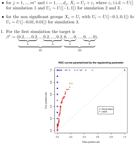
To better understand the difference of behaviour between the Lasso and the Group Lasso in terms of variables selection we also provide some kind of ROC curves. These curves are created by plotting the fraction of true positives (of the estimated parameter) out of the positive coefficients ofβ∗ for discretized values of the penalty parameter going from zero (completely dense solution)
up to the value where the first group of covariates enters the model (completely sparse solution). To ensure that we well detect each new inclusion of covariates, the discretization involves 10000
Simulation 1 2 3 4 5 6 7 8
s∗/p 20/120 20/120 20/120 40/240 10/60 20/120 40/140 60/160
G 12 12 12 12 12 12 14 16
m∗ 2 2 2 2 2 2 4 6
v 10 10 10 20 5 10 10 10
Mean Hit lasso (%) 86,9 99,4 99,95 66,27 87,6 95,9 78,79 54,16 Mean Hit group lasso (%) 100 100 100 98,5 100 100 100 98,8 Mean False positive lasso (%) 15,02 10,61 9,25 2,39 47,38 18,96 9,33 8,87 Mean False positive group lasso (%) 28,7 36,1 33,9 74 34,2 29,6 61,9 37,9 Mean Nonzero lasso 32,4 30,49 29,24 31,29 32,45 38,14 40,85 41,37 Mean Nonzero gp lasso 48,7 56,1 53,9 187,4 27,1 49,6 101,9 97,2 Mean Prediction error lasso 0,19 0,15 0,18 6,73 0,15 0,17 3,22 17,97 Mean Prediction error gp lasso 0,021 0,007 0,004 1,98 0,03 0,016 0,012 1,32
Mean Estimation error lasso 6,36 2,84 2,08 9,79 15,31 6,37 8,45 16,28 Mean Estimation error gp lasso 5,54 2,66 1,64 18,65 4,22 3,40 2,77 12,76
Table 1: Results of the simulations for the eight models
values of the penalty parameter. We plot the curves for each model considered. Three models are described below and the respective ROC curves are shown in Figures1,2 and3.
For each model we have
• forj= 1, ..., m∗ andi= 1, ..., d
j,Xi =Uj+εiwhereεi i.i.d∼U([−1,1]) and Uj∼U([0,1])
for simulation 1 andUj ∼U([−1,1]) for simulation 2 and 3 .
• for the non significant groupsXi =Ui with Ui ∼U([−0.1,0.1]) for simulation 1 and 2 and
Ui∼U([−0.01,0.01]) for simulation 3.
1. For the first simulation the target is
β∗= (0.2, ...,0.2 | {z } 5 , ...0.2, ...,0.2 | {z } 5 | {z } 10 ,0, ...,0 | {z } 5 , ...,0, ...,0 | {z } 5 | {z } 50 ). 0.0 0.2 0.4 0.6 0.8 1.0 0.0 0.2 0.4 0.6 0.8 1.0 False−positive rate T rue−positiv e r ate
ROC curves parametrized by the regularizing parameter
Group lasso Lasso
Figure 1: Simulation 1
β∗= (0.2, ...,0.2 | {z } 5 , ...0.2, ...,0.2 | {z } 5 | {z } 10 ,0, ...,0 | {z } 5 , ...,0, ...,0 | {z } 5 | {z } 100 ). 0.0 0.2 0.4 0.6 0.8 1.0 0.0 0.2 0.4 0.6 0.8 1.0 False−positive rate T rue−positiv e r ate
ROC curves parametrized by the regularizing parameter
Group lasso Lasso
Figure 2: Simulation 2
3. For the third simulation the target is
β∗= (0.2, ...,0.2 | {z } 5 , ...0.2, ...,0.2 | {z } 5 | {z } 10 ,0, ...,0 | {z } 5 , ...,0, ...,0 | {z } 5 | {z } 100 ). 0.0 0.2 0.4 0.6 0.8 1.0 0.2 0.4 0.6 0.8 1.0 False−positive rate T rue−positiv e r ate
ROC curves parametrized by the regularizing parameter
Group lasso Lasso
Figure 3: Simulation 3
The simulations clearly illustrate that contrary to the Lasso the Group Lasso includes not single covariates one after another but all the covariates which belong to the same group at the same time. The Group Lasso tends to include in priority the significant groups and then the non significant groups in such a way that for some values of the penalty parameter the rate of perfect selection can
be very close to one and even equal to one in some particular cases (see for instance Figure1). We can notice that the ROC curves for the Lasso follow at the beginning those of the Group Lasso and then fall below. The break in the curves of the Lasso illustrate a special feature of this estimator. Actually the number of covariates included in the model for the Lasso is restricted by the sample size whereas for the Group Lasso the restriction is given by the number of groups. That is why for the Lasso the number of true positives but also the number of false positives are smaller than those of the Group Lasso (once approximately 100 covariates are added in the model the Lasso stop including other ones). We can also notice that the Group Lasso is less stable than the Lasso in terms of variables selection. In fact a little change in the penalty parameter can substantially increase the number of false positives. This particular feature of the Group Lasso due to a group structure penalty is reflected in Table I with a rate of false positives larger for the Group Lasso in most of the cases. Thus Figures1, 2 and 3 confirm what has been previously deduced from the results presented in Table I. To conclude the Group Lasso seems to be more reliable than the Lasso to include the variables of interest but in return it tends to incorporate more false positives.
6
Conclusion
We consider the generalized linear model in high dimensional settings and use the Group Lasso estimator to estimate the regression parameter β∗ when the covariates are naturally structured into groups of variables and the true parameter is group sparse (just a few variables are relevant to explain the response). Under some assumptions on the sparsity ofβ∗, on the correlations between
the groups of covariates and on the tuning parameter of the estimator we state general oracle inequalities for estimation and error prediction for the Group Lasso estimator applied to generalized linear models. In the particular case of groups of size one, we provide original inequalities for the Lasso in the case of generalized linear models extending the results of Bunea [5] for logistic regression. Furthermore, we extend these results to other penalties such as the Elastic net. Then we compare the performances of the Lasso to the ones of the Group Lasso on simulated data. We show the improvement in terms of variables selection and prediction errror of the Group Lasso compared to the Lasso when the covariates are structured into groups. Moreover we illustrate on these simulated data the impact of the total number of groups, of the number of non zero groups and of the size of the groups on the performances of the Group Lasso. The conclusion is that the Group Lasso estimator behave well in a high dimensional setting under sparsity and group correlations assumptions. However the main drawback of the Group Lasso is that we need an a priori knowledge on the groups and it is not always possible.
A
Proof of Theorem
3.6
A.1
The main steps of the proof
The proof follows the guidelines in [4] or [13]. Using the mere definition of ˆβn, we have
Pnl( ˆβn) + 2rn Gn X g=1 p dgkβˆngk26Pnl(β∗) + 2rn Gn X g=1 p dgkβ∗gk2. (7) Hence we get Pl( ˆβn)−l(β∗)+ 2rn Gn X g=1 p dgkβˆngk2 6(Pn−P)l(β∗)−l( ˆβn)+ 2rn Gn X g=1 p dgkβ∗gk2. (8)
We decompose the empirical process into a linear part and a part which depends on the normalized parameterψ.
= (Pn−P)ll(β∗)−ll( ˆβn)+ (Pn−P)lψ(β∗)−lψ( ˆβn)
where
ll(β) :=ll(β, x, y) =−yβTx
and
lψ(β) :=lψ(β, x) =ψ(βTx).
From Proposition3.3 and Proposition3.5and by addingrnPGng=1
p
dgkβˆgn−β ∗g
k2 to both sides
of the inequality (8) we find, onA ∩ B, that
rn Gn X g=1 p dgkβˆng−β ∗g k2+P l( ˆβn)−l(β∗) 62rn Gn X g=1 p dg kβˆng−β ∗g k2+kβ∗gk2− kβˆngk2 +rn 2 εn. Ifg /∈H∗thenkβˆg n−β∗gk2+kβ∗gk2− kβˆngk= 0 and otherwisekβ∗gk2− kβˆgnk26kβˆng−β∗gk2. So
the last inequality can be bounded by 4rn X g∈H∗ p dgkβˆgn−β ∗g k2+ rn 2 εn. (9)
By the definition ofβ∗ we have Pl( ˆβ
n)−l(β∗) >0 and therefore X g /∈H∗ p dgkβˆng−β ∗g k263 X g∈H∗ p dgkβˆng−β ∗g k2+εn 2 i.e ˆβn−β∗∈S(3, εn
2 ). The next proposition provides a lower bound forP
l( ˆβn)−l(β∗)
.
Proposition A.1. On the eventA ∩ B we have
Pl( ˆβn)−l(β∗)>cnE fβnˆ (X)−fβ∗(X) 2 withcn := min |x|6L(9B+1 n) ψ′′(x) 2 . Proof. Pl( ˆβn)−l(β∗)=−EhE(Y|X)fˆ βn(X)−fβ∗(X) i +Ehψ′(fβ∗(X)) fβnˆ (X)−fβ∗(X) i +E " ψ′′ (fβ˜(X)) 2 fβnˆ (X)−fβ∗(X) 2#
where ˜βTX is an intermediate point between ˆβT
nX and ˜βTX given by a second order Taylor
expansion ofψ. Sinceψ′(fβ∗(X)) =E(Y|X) we find
Pl( ˆβn)−l(β∗)=E " ψ′′(fβ˜(X)) 2 fβnˆ (X)−fβ∗(X) 2# . Besides we have |β˜TX|6|β˜TX−β∗T X|+|β∗T X| 6 Gn X g=1 kβ∗g−βgk2kXgk2+ Gn X g=1 kβ∗gk2kXgk2.
Applying (H.1), we find
kXgk26L
p
dg.
Then using Lemma3.4and (H.3) we find
|β˜TX|6LM+LB a.s. (10) Furthermore,β∗ and ˆβ
n belongs to Λ which is a convex set. Therefore ˜β ∈Λ and ˜βTX ∈Θ a.s.
Thus we conclude Pl( ˆβn)−l(β∗)>cnE fβnˆ (X)−fβ∗(X) 2 wherecn := min {|x|6L(M+B)}∩Θ ψ′′(x) 2 .
From PropositonA.1and (9) we deduce that
rn Gn X g=1 p dgkβˆng−β ∗g k2+cnE ˆ βnTX−β ∗T X2 64rn X g∈H∗ p dgkβˆgn−β ∗g k2+ rn 2 εn. (11)
Then the end of the proof is similar to the end of the proof of Theorem 2.4 in [5]. Let Σ be the
p×pcovariance matrix whose entries areE(XkXj). We have EβˆT
nX−β
∗T
X2= ( ˆβn−β∗)TΣ( ˆβn−β∗).
Because conditionGS(3,εn2 , k) is satisfied we have
cn( ˆβn−β∗)TΣ( ˆβn−β∗)>cnk X g∈H∗ kβˆng−β ∗g k22− εn 2 . Then by using Cauchy-Schwarz inequality in (11) we find
rn Gn X g=1 p dgkβˆng−β ∗g k2+cnk X g∈H∗ kβˆgn−β ∗g k22 64rn sX g∈H∗ dg sX g∈H∗ kβˆng−β∗gk22+ (rn+ 1) εn 2 . Now the fact that 2xy6tx2+y2/tfor allt >0 leads to the following inequality
rn Gn X g=1 p dgkβˆng−β ∗g k2+cnk X g∈H∗ kβˆgn−β ∗g k22 64trn2γ∗+ 1 t X g∈H∗ kβˆng−β ∗g k22+ (rn+ 1) εn 2 . (12) Replacingtby 1 cnk in (12) we obtain Gn X g=1 p dgkβˆgn−β ∗g k26 4 cnk rnγ∗+ (1 + 1 rn )εn 2 . i.e kβˆn−β∗kR6 4 cnk rnγ∗+ (1 + 1 rn )εn 2 .
What is more p dminkβˆn−β∗k2,16 Gn X g=1 p dgkβˆng−β ∗g k2. This yields kβˆn−β∗k2,16 4 cnk√dmin rnγ∗+ 1 + 1 rn 1 2n√dmin . (13)
A similar argument could be made to prove
EβˆT nX−β ∗T X26 16 c2 nk rn2γ∗+ 2rn+ 1 cn εn 2 . (14)
Finally we conclude the proof using Proposition3.1.
A.2
Proof of Proposition
3.1
Proof. Let A > √2. We recall that we have made the assumption log(2nGn) 6 1. We deduce Proposition3.1from the two following lemmas.
Lemma A.2. Let
rn> 8 √ 2ALCL,B r log(2Gn) n ! ∨ 16A2LCL,B log(2Gn) n withA >1. Then
P{A}>1−2dmax(2Gn)1−A
2 . Lemma A.3. Let
rn>20AL max {|x|6Lκn}∩Θ|ψ ′ (x)| r2 log 2G n n whereA>1. Then P(B)>1−C(2Gn)−A 2 /2 where we recallκn:= 17B+ 2
n. We can notice thatP(B)n→∞−→ 1.
Thus if rn>AKL CL,B∨ max {|x|6Lκn}∩Θ|ψ ′ (x)|) r 2 log(2Gn) n
withKchoosen such that
rn>max (C1, C2, C3) where C1:= 8 √ 2ALCL,B r log(2Gn) n C2:= 16A2LCL,Blog(2Gn) n and C3:= 20AL max {|x|6Lκn}∩Θ|ψ ′ (x)| r 2 log 2Gn n
thenP(A ∩ B)>1−(2dmax+C)(2Gn)−A
2
A.3
Proofs of the technical lemmata
Proof of Lemma 3.2
Proof. Letθ∈Int(Θ) andYθ be a real random variable with density exp(θy−ψ(θ))F(dy). First
we prove that for allk∈N, there exists a constant Cθ>0 which depends onθsuch that E|Yθ|k6k!Ck
θ.
Thekthabsolute moment ofY
θ is thekthderivate ofHθ:=E(es|Yθ|) at 0. Lets∈Cbe given. We
have
Hθ(s) =
M+(s+θ) +M−(θ−s)
M(θ) where we defineM+ andM− as
M+: C −→ C z 7−→ Ry>0eyzF(dy) and M− : C −→ C z 7−→ Ry<0eyzF(dy).
M is analytic on ΩΘ :={z∈C: Re(z)∈Int(Θ)} and so does M+ and M−. Therefore Hθ :
s7−→E(es|Yθ|) is analytic onUθ:={s∈C: Re(s+θ)∈Int(Θ) and Re(θ−s)∈Int(Θ)}. Since
θ∈Int(Θ),Hθis analytic at the point 0 and hence the function is also holomorphic in a
neighbor-hood of 0. We recall the following result for analytic functions (see [28]).
Theorem: Iff is holomorphic on a domainΩofCthenf ∈ C∞(Ω) and if in additionΩis simply
connected then for all contourγ aroundz∈Ωwe have
f(n)(z) = n! 2iπ Z γ f(v) (v−z)n+1dv.
Using the previous theorem onHθ at 0 and taking γ as a circle with radius R centered in 0
(such thatHθ is holomorphic onD(0, R), of courseRdepends onθ) we obtain that for all k∈N
|Hθ(k)(0)|6 k! 2π Z γ Hθ(v) vk+1 dv 6 k! Rk sup |z|6R| Hθ(z)|. (15)
and the result follows withCθ := max 1,
1
R|z|sup6R|
Hθ(z)| !
. Thanks to assumption (H.2) we can apply (15) withθ=β∗TX and find that for allk∈N,
E |Y|k|X6k! Cβ∗TXk.
Finally (H.1) combined with (H.3) leads to
E |Y|k6k! sup
|θ|6LB
Cθ !k
and the result follows withCL,B:= sup |θ|6LB
Cθ.
Proof of Lemma 3.4
Proof. The proof is based on the convexity of the loss function and of the penalty, the main idea of the proof is similar to the one used by B¨uhlmann and van de Geer [4] for the Lasso to show consistency of the excess of risk. Definet:= M
M +PGng=1pdgkβˆgn−β∗gk2
NoticePGng=1pdgkβ˜g−β∗gk26M. By convexity ofβ→lψ(β) andβ→ kβk2combined with the
fact that ˆβn satisifies (7) we find
Pl( ˜β)−l(β∗)+ 2rn Gn X g=1 p dgkβ˜gk2 6(Pn−P)l(β∗)−l( ˜β)+ 2rn Gn X g=1 p dgkβ∗gk2.
On the eventATBwe have
Pl( ˜β)−l(β∗)+ 2rn Gn X g=1 p dgkβ˜gk2 6rn Gn X g=1 p dgkβ˜g−β∗gk2+rn εn 2 + 2rn Gn X g=1 p dgkβ∗gk2.
BecausePl( ˜β)−l(β∗)>0, by adding to both sides of the inequality 2rnPGng=1
p
dgkβ∗gk2and
by using the triangular inequality we have
Gn X g=1 p dgkβ˜g−β∗gk26 εn 2 + 4 Gn X g=1 p dgkβ∗gk2.
Therefore, using (H.3), we have
Gn X g=1 p dgkβ˜g−β∗gk26 εn 2 + 4B= M 2 . i.e. t Gn X g=1 p dgkβˆgn−β ∗g k26 M 2 and then the definition oftleads to
Gn X g=1 p dgkβˆng−β ∗g k26M.
Proof of Lemma A.2
Proof. We have P(Ac)6 Gn X g=1 P 1 n n X i=1 (YiXig−E(Y Xg)) 2 2 >r 2 n 4 dg 6 Gn X g=1 dg X j=1 P ( 1 n n X i=1 YiXi,jg −E Y X g j > rn 2 ) . (16)
Forj = 1, ..., dg andi= 1, ..., n, let
Wijg :=YiXi,jg −E YiXjg
.
The random variables{Wij}i=1,...,n are independant, identically distributed and centered and for
allm>2 E|Wg ij| m 6 m X k=0 k m E|YiXi,j|k(E|YiXi,j|)m−k
By using Jensen inequality we obtain E|Wg ij| m 62m max k=1,...,m E|YiXi,j|kE|YiXi,j|m−k .
For allk∈N, by (H.1) and Lemma3.2we have
E|YiXi,j|k6Lkk! (CL,B)k.
ThereforeE|Wg
ij|m6m!(2LCL,B)m. Hence the conditions are satisfied to apply Bernstein
concen-tration inequality [1] with K= 2LCL,B andσ2= 8(LCL,B)2. Thus we obtain
P 1 n n X i=1 Wijg > rn/2 ! 62 exp −nrn 16LCL,B + exp −nr2 n 32(2LCL,B)2 . (17)
Finally, from (16) and (17), we deduce thatP(Ac) is bounded by
2dmaxGn exp −nrn 16LCL,B + exp −nr2 n 32(LCL,B)2 . Therefore if rn>A216LCL,B log(2Gn) n ∨A8 √ 2LCL,B r log(2Gn) n withA >1 then PAC 62dmax(2Gn)1−A 2 .
Proof of Lemma A.3
Proof. The proof rests on the following Lemma
Lemma A.4. Let R >0 be given. Define
ZR:= sup PGn g=1 √ dgkβg−β∗gk 26R {|(Pn−P) (lψ(β∗)−lψ(β))|}. IfA>1 then P ZR>A5DLR r 2 log 2Gn n ! 6(2Gn)−A 2 (18) whereD:= max {|x|6L(R+B)}∩Θ n |ψ′(x)|o.
Proof. Letβ satisfyPGng=1
p
dgkβg−β∗gk26R. Notice that if we changeXi byX
′
i while keeping
the others fixed thenZRis modified of at most
2
nLRexp (L(R+B)). To see this let
Pn= 1 n n X j=1 1Xj,Yj and P′n= 1 n n X j=1,j6=i 1Xj,Yj + 1X′ i,Y ′ i then we have (Pn−P)(lψ(β∗)−lψ(β))−(P′n−P)(lψ(β∗)−lψ(β))
= 1 n lψ(β∗, Xi)−lψ(β, Xi)−lψ(β∗, X ′ i) +lψ(β, X ′ i) 6 1 n|ψ ′ ( ˜βTX i)||β∗TXi−βTXi|+ 1 n|ψ ′ ( ˜βTX′ i)||β∗ T Xi′−βTX ′ i| with ˜βTX
i which is an intermediate point between βTXi and β∗TXi (using a first order Taylor
expansion of the exponential function). Then, using the same argument as for (10), we have |β˜TXi|6LR+LB. Therefore (Pn−P)(lψ(β∗)−lψ(β))−(P′ n−P)(lψ(β∗)−lψ(β)) 6 2 nLR{|x|6Lmax(R+B)}∩Θ|ψ ′ (x)|= 2 nLRD.
We can apply McDiarmid’s inequality also called the bounded difference inequality.
Theorem. Let A a set. Assume g : AN →R is a function that satisfies the bounded difference
inequality sup x1,...,xn,x′i∈A |g(x1, ..., xn)−g(x1, ..., xi−1, x ′ i, xi+1, ..., xn)|6ci.
LetX1, .., Xn be independent random variables all taking values in the setA. Then for all t >0,
P{g(X1, ..., Xn)−Eg(X1, ..., Xn)>t}6e−2t2/Pni=1c 2
i.
We can apply McDiarmid’s inequality toZR and obtain
P(ZR−EZR>u)6exp − nu 2 2R2L2(D)2 ! . Therefore ifrn>ADLR r 2 log 2Gn n withA >0 then P(ZR−EZR>rn)6(2Gn)−A 2 . (19)
Now we have to bound the meanEZR.
Lemma A.5.
EZR64RLD
r
2 log(2Gn)
n .
Proof. First let us introduce two theorems. Let X1, ..., Xn independent random variables with
values in some spaceX andF a class of real-valued functions onX.
Theorem: Symmetrization theorem [27]. Letǫ1, ..., ǫn be Rademacher sequence independent
ofX1, ..., Xn andf ∈ F. Then E sup f∈F n X i=1 {f(Xi)−E(f(Xi))} ! 62E sup f∈F| n X i=1 ǫif(Xi)| ! .
Theorem: Contraction principle [12]. Letx1, ..., xnelements ofXandε1, ..., εnbe Rademacher
sequence. Consider Lipschitz functionsgi. Then for any function f andhin F, we have
E sup f∈F n X i=1 ǫi{gi(f(xi))−gi(h(xi))} ! 62E sup f∈F n X i=1 ǫi(f(xi)−h(xi)) !
Letǫ1, ..., ǫna Rademacher sequence independant ofX1, ..., Xnand letSR:= n β∈Rp:PGn g=1 p dgkβg−β∗gk26R o . Then by the Symmetrization theorem and the Contraction theorem (ψisD-lipschitz on the
com-pact setSR ) we have
EZR64DE sup β∈SR 1 n n X i=1 ǫi(β∗TXi−βTXi) ! 64DRE max g∈{1,...,Gn} 1 n n X i=1 ǫikX g ik2 p dg ! ,
by Holder inequality for the last bound. Now we are going to use the following theorem which is a consequence of Hoeffding inequality.
Theorem. Let X1, ..., Xn be independent random variables on X andf1, ..., fn real-valued
func-tions onX which satisfies for all j= 1, ..., p and alli= 1, ..., n
Efj(Xi) = 0, |fj(Xi)|6aij. Then E max 16j6p n X i=1 fj(Xi) ! 6p2 log(2p) max 16j6p v u u t n X i=1 a2 ij.
By applying this theorem we obtain
E max g∈{1,...,Gn} 1 n n X i=1 ǫik Xigk2 p dg ! 6L r 2 log(2Gn) n . Thus EZR64RLD r 2 log(2Gn) n . (20)
So we can conclude from (19) and (20) that ifA>1 then
P ZR>A5DLR r 2 log 2Gn n ! 6(2Gn)−A 2 (21) for allR >0. Split up ( β∈Rp: Gn X g=1 p dgkβg−β∗gk26M ) ,
whereM = 8B+εn, into two sets which are
E1= ( β : Gn X g=1 p dgkβg−β∗gk26εn ) , E2= ( β :εn6 Gn X g=1 p dgkβg−β∗gk26M ) ⊆ jn [ j=1 ( β : 2j−1εn< Gn X g=1 p dgkβg−β∗gk262jεn )
wherejn:=⌊log2(nM)⌋+ 1 is the smaller integer such that 2jnεn>M. We recall that
νn(β, β∗) := (Pn−P) (lψ(β∗)−lψ(β)) PGn g=1 p dgkβg−β∗gk2+εn