econ
stor
www.econstor.eu
Der Open-Access-Publikationsserver der ZBW – Leibniz-Informationszentrum Wirtschaft
The Open Access Publication Server of the ZBW – Leibniz Information Centre for Economics
Nutzungsbedingungen:
Die ZBW räumt Ihnen als Nutzerin/Nutzer das unentgeltliche,
räumlich unbeschränkte und zeitlich auf die Dauer des Schutzrechts
beschränkte einfache Recht ein, das ausgewählte Werk im Rahmen
der unter
→ http://www.econstor.eu/dspace/Nutzungsbedingungen
nachzulesenden vollständigen Nutzungsbedingungen zu
vervielfältigen, mit denen die Nutzerin/der Nutzer sich durch die
erste Nutzung einverstanden erklärt.
Terms of use:
The ZBW grants you, the user, the non-exclusive right to use
the selected work free of charge, territorially unrestricted and
within the time limit of the term of the property rights according
to the terms specified at
→ http://www.econstor.eu/dspace/Nutzungsbedingungen
By the first use of the selected work the user agrees and
declares to comply with these terms of use.
Jaschke, Stefan; Stahl, Gerhard; Stehle, Richard
Working Paper
Evaluating VaR Forecasts under Stress The
German Experience
CFS Working Paper, No. 2003/32
Provided in Cooperation with:
Center for Financial Studies (CFS), Goethe University Frankfurt
Suggested Citation: Jaschke, Stefan; Stahl, Gerhard; Stehle, Richard (2003) : Evaluating VaR
Forecasts under Stress The German Experience, CFS Working Paper, No. 2003/32, http://
nbn-resolving.de/urn:nbn:de:hebis:30-10376
This Version is available at:
http://hdl.handle.net/10419/72644
No. 2003/32
Evaluating VaR Forecasts under Stress –
The German Experience
CFS Working Paper No. 2003/32
Evaluating VaR Forecasts under Stress – The German
Experience
*
Stefan Jaschke
1
, Gerhard Stahl
1
,
Richard Stehle
2
October 2003
Abstract:
We present an analysis of VaR forecasts and P&L-series of all 13 German banks that used
internal models for regulatory purposes in the year 2001. To this end, we introduce the notion
of well-behaved forecast systems. Furthermore, we provide a series of statistical tools to
perform our analyses. The results shed light on the forecast quality of VaR models of the
individual banks, the regulator's portfolio as a whole, and the main ingredients of the
compu-tation of the regulatory capital required by the Basel rules.
JEL Classification: K23, G28
Keywords: banking supervision, VaR, exploratory data analysis, backtesting
*
The first two authors point out that the views expressed herein should not be construed as being
endorsed by the BaFin.
In animportantregulatory innovation theBasel Committeeon BankingSupervisionhas
allowedforbankstousetheirowninternalmodels{ so-calledValue-at-Risk (VaR)
mod-els { for calculating the regulatory capital cushion needed to cover the market risk of
open positionsinan institute'stradingbook. Comparedwith thestandardizedmethods
the internal models approach oers a whole bunch of advantages within the process of
risk management, i.e., in measuring, monitoring and managing market risk for trading
portfolios. These advantagesinclude theconvergenceof economicand regulatory capital
(Matten; 2000), the avoidance ofduplicatedeorts forinternaland regulatory risk
mea-surement and, among others, the signaling of competence to the market, especially to
ratingagencies, by regulatoryapproval ofan internal model.
Lookingbackon theyear2001 we recognize thatanumberofsevereeventstook place
in the nancial markets. Not only the terrorist attack from September 11, but also a
signicant numberof interestrate decisionsofcentralbanks,theEnroncase, the
contin-uingdemiseofthe\neweconomy",andothers, tookplace. Obviously,mostoftheevents
mentionedwere unpredictablebutdramaticinsome sense. That the year2001 was
spe-cialisalso highlightedbythefactthat13 German banksproduced33 VaR exceptionsin
the year 2001 while14 German banksproduced17 VaR exceptions in 2002. Given the
turbulences of that year, it is natural to ask whether the forecast quality of VaR
mod-els over the year 2001 turned out to be satisfactory. A second question is whether the
portfolios of the supervisedbanks behave similarlyand whether the similarityincreases
in stress periods. Put in another way, how well is the supervisor's portfolio diversied
and is this aected by the special events of the year 2001? This is the rst article to
provide a detailedempirical analysis of (1)the performanceof the actualVaR forecasts
of all German banks that used internalmodelsfor regulatory purposes in 2001 and (2)
the interrelations among the prots and losses (P&L) of these banks, especially during
thestressperiods. Insofar,itiscomparableto theempiricalanalysisofsimilardatafrom
six US banks by Berkowitz and O'Brien (2002). The methodology employed, however,
dierssignicantly.
TheBasel paperon backtestingdescribesin-depththe regulatoryrequirementsonthe
forecast quality of the trading book asa whole in order to ensurean adequate
calcula-tion of regulatorycapital (Basel Committee on BankingSupervision;1996b). Numerous
publications reect VaR forecast evaluation, starting with Kupiec (1995), who points
out thelackof statistical powerof a backtesting that isbased on a binomial test
statis-tic. Crnkovic and Drachman (1996) propose the use of the Kuiper statistic, which is
a goodness-of-t type statistic based on the whole forecast distribution. Christoersen
(1998) draws the attention to backtesting based on specication tests, focussing on the
independence property to evaluate forecast quality. Inspiredby the ideasof Rosenblatt
(1952), Berkowitz (2000) proposed an approach that relies on conditioned forecast
dis-tributions. This is very much inthe spiritof the papers ofDawid, see(Dawid; 1982a,b,
1984, 1986;Seillier-Moiseiwitschand Dawid; 1993). Thisagainis inuencedbythe
liter-atureonwheatherforecasting(Murphyand Winkler;1987,1992). Adetailedoverviewof
backtesting issuesis given by Overbeckand Stahl (2000). The empiricalanalysis of the
forecastqualityinthispaperisinthespiritofDawid'sforecastevaluation. Thefactthat
rigorous justication of our approach is given in the appendix. The methodology used
to analyze the joint behavior of all banks includes a measure of co-movement and
sev-eral stress variablesusedto denestress periods. Finally,we consider howdistributional
parameters changeconditional onstress.
Beforedescribingthedataset,letusintroducesomenotation. WedenotebyVaR (
t
;)
theValue-at-Riskofaportfolio
t
,giventhelevelofsignicance. Withintheframework
of theBaselCommittee, issetto 99%. The VaRnumberVaR (
t
;) at timetdenotes
the quantileof thedistributionof thehypothetical, orclean,P&L
C t =v t+1 ( t ) v t ( t ); (1) where v t
() is the value of a given portfolio at time t. The random variable v
t+1 (
t )
denotes the at time t frozen portfolio, evaluated at prices of time t+1. The VaR is
interpreted as an upper boundof losses that might be surpassed only with probability
1 . Inthesequel wewillusethe shorthandnotation V
t
to denote VaR (
t
;99%).
Withinanobservation periodof 250 tradingdays2.5 violationsof theforecasts V
t are
to be expected on theaverage. Hence,if too manyviolationsoccur there isgoodreason
to doubt that the internal model's level of signicance is correctly covered. In order to
ensure a suÆcient forecast quality, the Basel Committee tied theamount of the capital
requirementstothenumberofVaRexceptionsofthemodel(BaselCommitteeonBanking
Supervision;1996a).
Itisofgreatpracticalimportancetonotethatfreezingtheportfolio{asstatedin(1){
isnotimperative. TheBaselCommitteealsoacknowledgesbacktestingVaRthatisbased
on actualtradingoutcomes. Inthatcase changes oftheportfoliocompositionduringthe
holdingperiod,feesetc. aresuperimposedonthehypotheticalP&L.Fromastatistician's
pointofview,thejudgmentofforecastqualityshouldbebasedonthehypotheticalP&L,
(1), because the VaR forecast assumes a static portfolio by construction. From a risk
managers point of view, however, the actualor economic P&L is actively managed and
reported. Obviouslybothwaystotacklethebacktestingproblemhavetheirintrinsic
mer-its. German legislationprescribesabacktestingbased on (1),whereastheUS legislation
admitsto basethebacktestingontheeconomicP&L,see(BerkowitzandO'Brien;2002).
2. Description of the Data Set
The data set considered here contains data from all thirteen German banks that used
internal models for regulatory purposes in the year 2001. The data set for each bank
consists of rst, VaR forecasts and second, the so-called clean, orhypothetical P&L for
all 253 trading days of theyear 2001. Most ofthe followingguresand tablesare based
on the normalized P&L and VaR time series. I.e., they are divided by the banks' full
sample standarddeviation of P&L to insurecondentiality.
Table1showssummarystatisticsofeach bank'sdata. ThecoeÆcientofvariation(i.e.,
the ratio of the standard deviation and the mean) of VaR in column 5 shows that for
the majority of the banks the variabilityof the VaR is relatively smallcompared to its
name oflosses VaR variationofVaR lossexceedingVaR A 22.51 3.15 1.83 2.68 0.84 0.00 B 6.48 0.00 2.62 4.51 0.29 1.34 C 5.98 0.61 2.18 4.05 0.14 0.00 D 5.58 0.19 2.55 3.29 0.26 0.00 E 7.79 0.43 2.56 1.69 0.87 0.56 F 16.99 2.10 3.52 2.11 0.52 1.63 G 3.71 0.20 2.42 2.15 0.23 0.24 H 5.72 0.01 2.12 2.25 0.23 1.49 I 15.03 1.58 4.55 1.07 0.87 0.73 J 4.04 0.67 2.98 3.03 0.39 0.37 K 5.28 0.00 2.24 2.20 0.11 1.37 L 4.57 0.22 2.75 3.85 0.20 0.00 M 3.35 0.12 2.45 2.58 0.18 0.00
Table1:Summarystatisticsofstandardizeddata. Thecolumnsgivekurtosis,
skew-ness,minusthe1%-quantileoftheP&L,theaverageVaR,thecoeÆcientofv
ari-ation oftheVaR,andtheaveragesizeofthelossexceedingVaR.BothP&Land
VaR arere-normalizedinsuch a way thatthestandarddeviation ofthe P&Lis
1 forall banks.
exceedingVaR,i.e., theestimate oftheexpectedshortfallE[ C
t V t j C t >V t ]. Note,
thatforthestandardnormaldistribution,theexpectedshortfallisapproximately0.34for
the99%condencelevel. The comparativelylargeaveragelosses exceedingVaR indicate
thepresenceofoutliers. Threeoutofthethirteenbankshadmorethanfourviolationsand
onlyfour had no violationsat all. For reasons of condentiality,theindividualnumbers
of violationsarenotreported here.
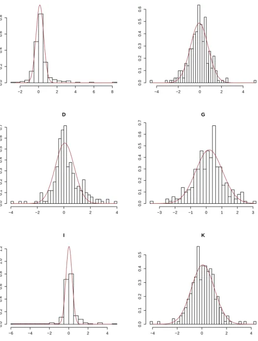
The six histogramsin gure 1 are representative forthe dataset. The histogramsare
fairlysymmetric,whichis inlinewiththeskewness intable 1. Takingintoaccount that
the data are standardized, the large range of the x-axis for bank I shows the presence
of extreme outliers. This suggests the use of robust estimates of locationand scale. To
be specic, we use the median F
1 0:5
as an estimate for the location parameter and the
interquartile range F 1 0:75 F 1 0:25
as an estimate of the scale parameter. In gure 1 the
tted normaldensitiesusethemedianasa robustestimator ofthemeanand normalized
interquartile range (F 1 0:75 F 1 0:25 )=( 1 0:75 1 0:25
) is a robust estimator of the standard
deviation. ( 1 0:75 1 0:25
1:349istheinterquartilerangeofthestandardnormal
distribu-tion.) ThisimprovestherepresentationofthebulkofthedatabyaGaussiandistribution.
Furthermore,itisevidentthatthelargeexcesskurtosis andskewnessofbank Iiscaused
bya fewextremeoutliers relative to thenormal distribution.
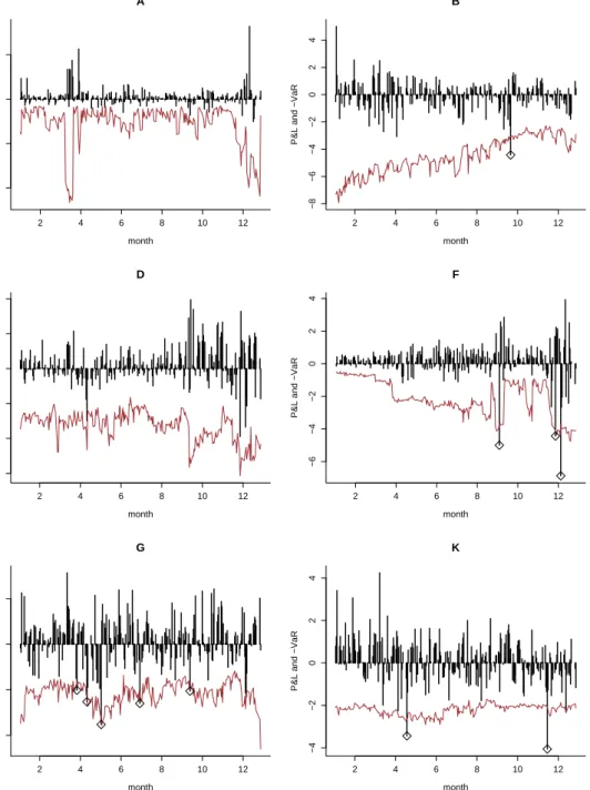
Figure2showsthetimeseriesof P&Land VaR oftheselected institutes. Ascan be
seen from banksBand F, forexample, itisnot reasonableto assumestationarity ofthe
P&L and VaR timeseries. Hence,the summary statisticsgiven intable 1 as wellasthe
histogramsingure 1 areto beinterpretedwithcare. BanksB, D,and F give a picture
A
−2
0
2
4
6
8
0.0
0.2
0.4
0.6
0.8
B
−4
−2
0
2
4
0.0
0.1
0.2
0.3
0.4
0.5
0.6
D
−4
−2
0
2
4
0.0
0.1
0.2
0.3
0.4
0.5
0.6
0.7
G
−3
−2
−1
0
1
2
3
0.0
0.1
0.2
0.3
0.4
0.5
0.6
0.7
I
−6
−4
−2
0
2
4
0.0
0.2
0.4
0.6
0.8
1.0
1.2
K
−4
−2
0
2
4
0.0
0.1
0.2
0.3
0.4
0.5
Figure 1:Histograms of the P&L and tted normal densities. The mean and
standard deviation of the tted normal density are estimated robustly by the
2
4
6
8
10
12
−
10
−
50
5
A
month
P&L and
−
VaR
2
4
6
8
10
12
−
8
−
6
−
4
−
20
2
4
B
month
P&L and
−
VaR
2
4
6
8
10
12
−
6
−
4
−
20
2
4
D
month
P&L and
−
VaR
2
4
6
8
10
12
−
6
−
4
−
20
2
4
F
month
P&L and
−
VaR
2
4
6
8
10
12
−
4
−
20
2
G
month
P&L and
−
VaR
2
4
6
8
10
12
−
4
−
20
2
4
K
month
P&L and
−
VaR
Figure 2:Time series of P&L and -VaR. The vertical dotted lines denote the date
0.0
0.2
0.4
0.6
0.8
1.0
0.0
0.2
0.4
0.6
0.8
1.0
Lorenz curve of the average VaR
ranking in the sorted set
cumulative proportion
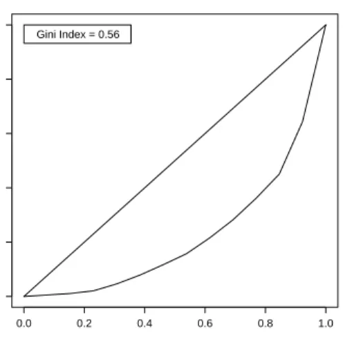
Gini Index = 0.56
Figure 3:Lorenz curve of the average VaR of all banks. The largest three banks
interms ofaverage VaR capture61%of theaggregated average VaRs.
Asthedescriptivestatisticsshow,bankstendto beconservative inthesensethatthey
overestimatetheirVaR.ThetraÆclightapproachis relatedto aone-sidedlossfunction,
asreportedintable 1. Hence,thisbacktest doesnotrecovertheinformationinthedata
about forecast quality of a VaR-model as a whole. In the next section we will have a
closer lookat forecast qualityusingmore powerfultools.
WeconcludethissectionwiththeLorenzcurveingure3,whichdepictsthe
concentra-tion ofrisksamong thethirteenbanksand givessomecomplementaryinformationabout
therelative \size"of thebanks.
3. Analyzing VaR-Forecasts for Each Bank Individually
In their paper on backtesting, the Basel Committee on Banking Supervision (1996b)
encourages institutes to apply backtesting procedures beyond the so-called traÆc light
approach. In this section, we make proposals for possible renements. The proposed
toolshavebeenusedbytheBundesanstaltfurFinanzdienstleistungsaufsicht(BaFin),the
Germansingleregulatorforintegratednancialservicessupervision,foracoupleofyears.
In the following, we use the term prediction-realization pair for the class of objects
((F t );C t ), where F t
denotes the whole forecast distribution and (F
t
) a parameter
thereof, e.g., a quantile, orthe distributionas awhole (=id). The summary statistics
from section 2 give a description of the prediction-realization pairs(V
t
;C
t
). In order to
evaluate theforecast qualityof VaR modelswe introduce astatistical modelthat allows
to incorporateadditionalinformationfrom theprediction-realizationpairs (F
t
;C
t ).
Thetime plotsdisplayed ingure2 showthatneither of thetime seriesC
t
nor V
t are
stationary. Fortheevaluationofaforecastmodelitisnaturalto lookfortransformations
T suchthatthetimeseriesT((F
t
);V
t
T(F t ;C t )=F t (C t ) (2)
isusedasastartingpoint. A forecastsystemisconsidered\good" (Dawid;1984, p.281),
ifthevaluesF
t (C
t
) are independentand uniformlydistributed,i.e., F
t (C
t
) iidU[0;1].
Thiscorrespondsto theconcepts\well-calibration"and\renement" (=\resolution")
asusedintheliteratureonweatherforecasting(MurphyandWinkler;1987,1992)insofar
as the condition F
t (C
t
) U[0;1] essentially means \well-calibration" and the temporal
independence of F
t (C
t
) is related to \renement" (Dawid; 1986; Seillier-Moiseiwitsch;
1993).
While it has been proposed (Berkowitz; 2000) that banks should report the realized
probabilities F
t (C
t
) to the supervisory authorities, the current rules only require the
reportingofC t andV t = F 1
(0:01). Theforecastevaluation(backtesting) aslaiddown
inthe BaselAmendment isdened intermsof theVaR-exceptions
T(V t ;C t )=1 fV t C t g : (3)
The drawbacks of this approach are discussedby Kupiec (1995). Seealso Lopez (1999)
and (Jorion;2001, chapter 6).
Inthis section,we suggestan approach that bridges thegap betweenthe information
presentedbytheprediction-realizationpairs(2)and(3) . Inthedelta-normalRiskMetrics
framework,theVaR-forecast V
t
is relatedtotheforecastofthestandarddeviationofthe
P&L, t ,as V t =z t ; (4)
where z is the standard normal 99%-quantile, (z) = 0:99. There, the standardized
returns aredenedas
R t :=T(C t ;V t )=zC t =V t ; (5)
(Longerstaey; 1996, chapter 11) and are iid standard normal under the specic model
assumptionsof thedelta-normal approach. Thisdenition(5)of standardizedreturns is
useful even if (4) is invalid. A rigorousjustication of this statement and thefollowing
approach isprovidedintheappendix. Thestandardized returnsprovidethe basisofthe
forecast evaluation inthispaper.
We callaVaR forecast systemwell-behaved
3 if R t iidF 2U G " ; where U "
is the "-neighborhood of the set of Gaussian distributionswith respect to the
Kolmogorovdistance intheset ofprobabilitydistributions:
U G " :=fFjsup x jF(x) (; 2 )(x)j";F ispdf;2R; 2 2(0;1)g (6) 3
Notethat\well-behaved"is nottobeinterpreted as\favorable fromasupervisorypointofview". It
asHuber'sgrosserror modelinthe literatureofrobuststatistics, F G " :=fFjF =(1 ")(; 2 )+"H;2R; 2 2(0;1)g; (7)
where H is an arbitrary probabilitydistribution, isan important subset of U
G " . In fact, if F 2 F G "
, then exist , , and H such that F = (1 ")(;
2
)+"H. Then the
Kolmogorovdistance betweenthedistributionsF and (;
2 ) is d(F;(; 2 ))=sup x2R jF(x) (; 2 )(x)j; =" sup x2R jH(x) (; 2 )(x)j ="d(H;(; 2 ))":
In terms of the P-P plot of F against normal, which plotsF(x) against (;
2
)(x) for
x 2 R, this means that the graph is (vertically) within an "-band of the diagonal. On
theotherhand,anypointwithinthatbandcanbereachedbythegraphofadistribution
F 2U
G "
.
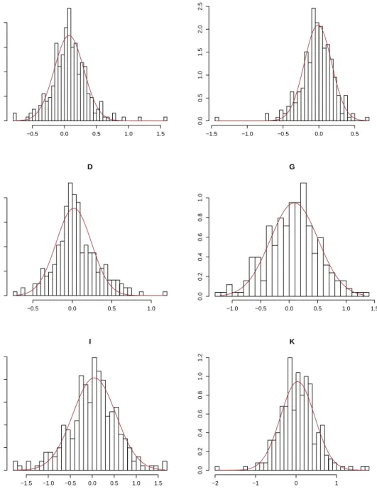
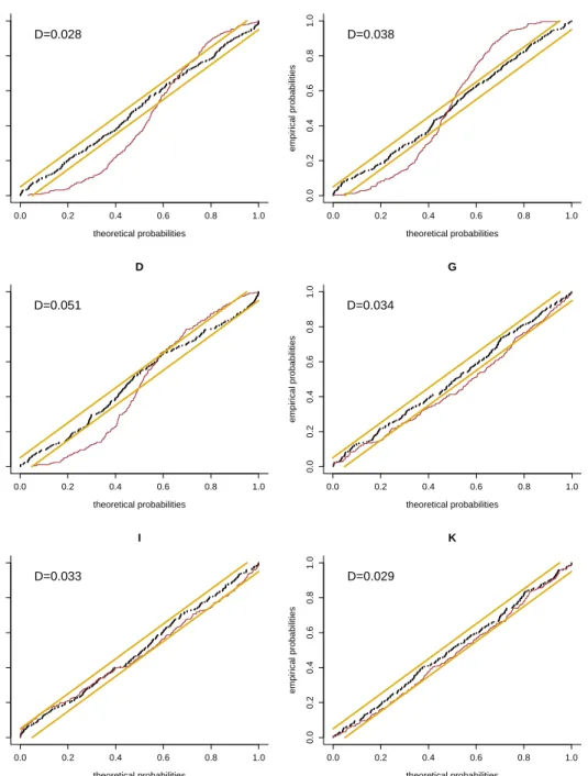
TheGaussiandistributionwithrobustlyestimatedparametersts(byeye)remarkably
wellto thecenter of standardized returns R
t
,seegure 4. The P-Pplot against normal
(gure5)alsoshowsthatthedistributionsofthestandardizedreturnsarerelativelyclose
tonormal,inthesensethattheyareintheclassU
G "
with"=0:05. (Infact,theempirical
distributionsof allbanksare inthisclass.)
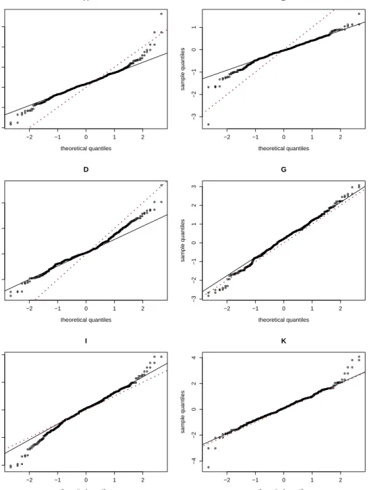
The P-P plot (and the Kolmogorov distance) does not detect large deviations from
normalityaslong asthey happen withsmall probabilities. A better pictureof thet in
the tails is provided by the Q-Q plot of F against normal, which plots F
1 (t) against 1 (; 2
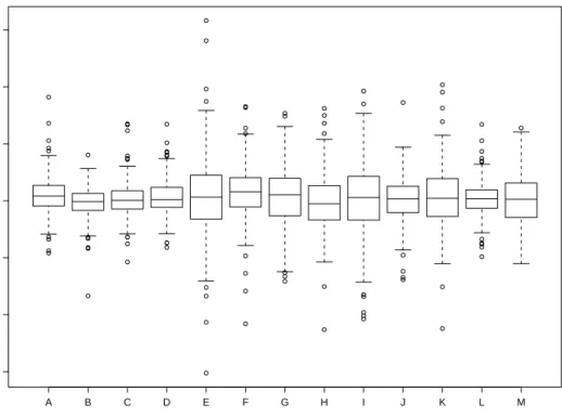
)() for 2(0;1), see gure 6. Anotherdisplaywith emphasis on the tails is
theboxplot, seegure7.
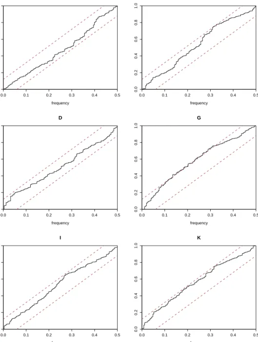
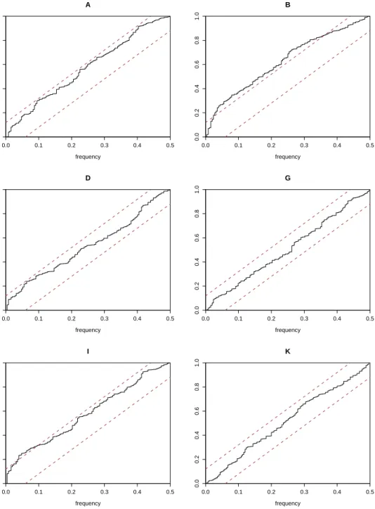
Diagnosticsthatillustrateserial(in-)dependenceofR
t
areprovidedbythecumulative
periodogramappliedtobothstandardizedreturnsandtheirabsolutevalues. Asexpected,
gure8showsthatthereisnosignicantautocorrelationinthestandardizedreturnseries.
Unliketheabsolutereturnsofmanynancialsecurities,theabsolutestandardizedreturns
of the banking books show no marked heteroscedasticity, see gure 9. Possibly reasons
are that the banks' VaR-forecasts successfully predict some of the heteroscedasticity of
their P&L-series. Another possible reason could be that the risk control limit system
lters outsome of theheteroscedasticityofthe originalreturns.
Thesetofwell-behavedVaR-forecastscontainsforecasts thatgrosslyover-or
underes-timate therespectivequantile. Undertheassumptionthatstandardizedreturnsarei.i.d.
standard normal, the inverse of the standard deviation of R
t
can be interpreted as the
recalibration factor. Thelargeritis,themorethebankoverestimatesitsVaR.Wewillcall
a forecast well-calibrated,iftherecalibration factor equals one
4
. Instead of looking only
at theempiricalstandard deviationof the standardized returnR
t
,one can alternatively
4
The relation between this notion of \well-calibration" and its denition in the forecast evaluation
literature can be made rigorous in more general settings than the delta-normal method, which is
A
−0.5
0.0
0.5
1.0
1.5
0.0
0.5
1.0
1.5
2.0
B
−1.5
−1.0
−0.5
0.0
0.5
0.0
0.5
1.0
1.5
2.0
2.5
D
−0.5
0.0
0.5
1.0
0.0
0.5
1.0
1.5
2.0
G
−1.0
−0.5
0.0
0.5
1.0
1.5
0.0
0.2
0.4
0.6
0.8
1.0
I
−1.5
−1.0
−0.5
0.0
0.5
1.0
1.5
0.0
0.2
0.4
0.6
0.8
1.0
K
−2
−1
0
1
0.0
0.2
0.4
0.6
0.8
1.0
1.2
Figure 4:Histogramsofthe standardizedreturnandttednormaldensity. The
meanandstandarddeviationofthettednormaldensityareestimatedrobustly
0.0
0.2
0.4
0.6
0.8
1.0
0.0
0.2
0.4
0.6
0.8
1.0
A
theoretical probabilities
empirical probabilities
D=0.028
0.0
0.2
0.4
0.6
0.8
1.0
0.0
0.2
0.4
0.6
0.8
1.0
B
theoretical probabilities
empirical probabilities
D=0.038
0.0
0.2
0.4
0.6
0.8
1.0
0.0
0.2
0.4
0.6
0.8
1.0
D
theoretical probabilities
empirical probabilities
D=0.051
0.0
0.2
0.4
0.6
0.8
1.0
0.0
0.2
0.4
0.6
0.8
1.0
G
theoretical probabilities
empirical probabilities
D=0.034
0.0
0.2
0.4
0.6
0.8
1.0
0.0
0.2
0.4
0.6
0.8
1.0
I
theoretical probabilities
empirical probabilities
D=0.033
0.0
0.2
0.4
0.6
0.8
1.0
0.0
0.2
0.4
0.6
0.8
1.0
K
theoretical probabilities
empirical probabilities
D=0.029
Figure 5:P-Pplotofthe distributionofthestandardizedreturnagainsta
stan-dardnormal(dottedline)andattednormaldistribution(fatdotted
line). The mean and standard deviation of the tted normal distribution are
chosentominimizetheKolmogorovdistancetotheempiricaldistribution
func-tion. D is that minimal distance. The dashed lines are the envelope of all
−2
−1
0
1
2
−
2
−
1
0123
A
theoretical quantiles
sample quantiles
−2
−1
0
1
2
−
3
−
2
−
10
1
B
theoretical quantiles
sample quantiles
−2
−1
0
1
2
−
1
012
D
theoretical quantiles
sample quantiles
−2
−1
0
1
2
−
3
−
2
−
1
0123
G
theoretical quantiles
sample quantiles
−2
−1
0
1
2
−
4
−
20
2
4
I
theoretical quantiles
sample quantiles
−2
−1
0
1
2
−
4
−
20
2
4
K
theoretical quantiles
sample quantiles
Figure 6:Q-Qplotofthestandardizedreturn. Thedottedlinedenotesthestandard
normal distribution, the solid line denotes the normal distribution with mean
and variance estimated from the sample, and the small circles represent the
A
B
C
D
E
F
G
H
I
J
K
L
M
−
6
−
4
−
20
2
4
6
Figure 7:Boxplot of the standardized return. The box shows the interquartile
range and the middle line the median. The \whiskers" are drawn 1.5 times
the interquartile range away from the box. Any point further away is shown
individually.
lookat dierentestimates
^ p (R ):= 1 T T X t=1 jR t j p ! 1=p =c p (8)
ofthestandarddeviationofR
t forpowersp>0. (c p istheconstantc p =(EjXj p ) 1=p with
X beingstandardnormal.) Usingsmallerpowersp<2givesmorerobustestimatesthan
the usualestimate of thestandard deviation. Usinglarger powers p>2 givesestimates
of the standard deviation that are more sensitive, i.e., more dependent on the extreme
values of R
t
, than the usual estimate of the standard deviation (p= 2). By lookingat
^ p
(r) for dierent powers p, one can observe whether banks are well-calibrated at the
center orat thetails,respectively.
5
Table2showsestimatesof therecalibrationfactor,aswellasp-valuesfromtestingthe
hypothesis that this factor equals 1. These results are further illustrated by gure 10,
5
Notethat thevariousdierent^
p
(r)are estimatesof thestandarddeviationofR
t
onlyifthe R
t are
0.0
0.1
0.2
0.3
0.4
0.5
0.0
0.2
0.4
0.6
0.8
1.0
frequency
A
0.0
0.1
0.2
0.3
0.4
0.5
0.0
0.2
0.4
0.6
0.8
1.0
frequency
B
0.0
0.1
0.2
0.3
0.4
0.5
0.0
0.2
0.4
0.6
0.8
1.0
frequency
D
0.0
0.1
0.2
0.3
0.4
0.5
0.0
0.2
0.4
0.6
0.8
1.0
frequency
G
0.0
0.1
0.2
0.3
0.4
0.5
0.0
0.2
0.4
0.6
0.8
1.0
frequency
I
0.0
0.1
0.2
0.3
0.4
0.5
0.0
0.2
0.4
0.6
0.8
1.0
frequency
K
Figure 8:Cumulative periodogram of standardized returns. White noiseis
char-acterized by equal probabilities for all frequencies, which shows as a straight
line in the cumulative periodogram. 95%-condence bands are given for the
0.0
0.1
0.2
0.3
0.4
0.5
0.0
0.2
0.4
0.6
0.8
1.0
frequency
A
0.0
0.1
0.2
0.3
0.4
0.5
0.0
0.2
0.4
0.6
0.8
1.0
frequency
B
0.0
0.1
0.2
0.3
0.4
0.5
0.0
0.2
0.4
0.6
0.8
1.0
frequency
D
0.0
0.1
0.2
0.3
0.4
0.5
0.0
0.2
0.4
0.6
0.8
1.0
frequency
G
0.0
0.1
0.2
0.3
0.4
0.5
0.0
0.2
0.4
0.6
0.8
1.0
frequency
I
0.0
0.1
0.2
0.3
0.4
0.5
0.0
0.2
0.4
0.6
0.8
1.0
frequency
K
A 1:670 1:614 1:480 B 2:162 2:053 1:849 C 1:899 1:832 1:659 D 1:805 1:690 1:552 E 0:825 0:786 0:710 F 1:147 1:129 1:055 G 0:938 0:946 0:940 H 1:074 1:037 0:980 I 0:831 0:808 0:769 J 1:466 1:403 1:296 K 1:004 0:992 0:944 L 1:838 1:765 1:625 M 1:143 1:110 1:090
Table2:Robust and sensitive estimates of the recalibration factor. The
esti-mates 1=^
p
(r) (see equation (8) ) of the recalibration factor are computed for
powers p 2 f0:5;1;2g. p-values for the corresponding null hypothesis that the
recalibration factor is one (i.e., that the R
t
are iid standard normal) are
com-puted byMonte-Carlo simulation. Signicanceat the 5%-level isshownbyone
star and signicance at the1%-levelwith two stars.
showing the recalibration factor estimated with the empirical standard deviation (p =
2) and the interquartile range, respectively. Note that banks E and I are consistently
underestimating its VaR. Alsonote that all banks are close to the line with slope 0.84
and intercept 0. This means rst, that the distributions of their standardized returns
have slightly heavier tails than the normal distribution. Second, the estimate of the
recalibration factor dependsonlymoderatelyon howrobustlyit isestimated.
Thelocalaveragesoftheabsolutevaluesofthestandardizedreturns(=estimatesofthe
inverseof therecalibrationfactor usingp=1)ingure 11showonlymoderate variation
intime, except forsome unpredictedabsolutereturns ofbanksBand I.
Insummary,thestandardizedreturnseriesofalltradingbooksareremarkablycloseto
being\well-behaved"asdenedinthissection. I.e.,theyareclosetonormalinthesense
of the Kolmogorov distance and there areno obvious temporal dependencies. This isin
starkcontrasttotheconclusionsdrawnbyBerkowitzandO'Brien(2002). Theyshowthat
theVaR-forecastsofthesixUSbanksconsideredareinferiortothatofasimple
\reduced-form" model,i.e., a univariatetime seriesmodel applied directly to the individualP&L
series. Their conclusion is that the banks' forecasts \did not adequately reect changes
inP&Lvolatility". Theconclusionfromtheempiricalevidence presentedinthissection,
however,isthattheVaR-forecastsoftheconsideredGermanbanksare\essentiallyOK":
the conservative VaR-forecasts of most banks can be corrected by simply re-calibrating
them. Much of the non-normality of the standardized return distributions in the view
of thetail-sensitivegraphs(gure 6) can be traced back to theessentially unpredictable
A
B
C
D
E
F
G
H
I
J
K
L
M
1.0
1.2
1.4
1.6
1.8
2.0
2.2
0.8
1.0
1.2
1.4
1.6
1.8
robust estimate
usual estimate
Figure 10:Sensitiveand robustestimates ofthe recalibration factor,estimated
withthe usualestimateofthe standard deviation(p=2) andthe
in-terquartile range. BankstowardsnortheastoverestimatetheirVaR.Banks
towards southeast have outliers orheavy tails. The black linerepresentsthe
bestlinear t withintercept 0. Itsslopeis 0:84.
4. Analyzing P&L Series For All Banks Simultaneously
The analysis of themodel qualityfor banksindividuallygivesthe supervisor important
information concerning the supervision of each bank. On the other hand, the analysis
of cross-sectionalinterrelationsof thebanks,e.g.,co-movements, is atleastasimportant
becauseitshedslightontheaspectsof systemicrisk. Fromtheregulator'spointofview,
two adverse scenarios are important. The rst case is when the regulator's portfolio is
notwell-diversiedinthe sensethatall portfoliosbehave similarly. A more specic case
is,when portfoliosbehavesimilarlyinperiodsofstress.
Theeconomic relevanceof theP&Lseriesdominatesthatof theVaRnumbers. Hence
we perform our cross-sectional analysis from a P&L point of view. A natural point to
start withis thecalculation of correlations, say. Yet tablesforcross correlationsquickly
get unmanageable for larger numbers of banks. Instead of lookingat m(m 1)=2= 78
cross correlations, itmay be more usefulto look at them=13 correlationsbetweenthe
individualP&L seriesand an aggregated P&L-series. Theidentity
m X j=1 cov(C i ;C j )=cov(C i ; m X j=1 C j )=cov(C i ; X j6=i C j )+var(C i )
motivates to considerthe covariances cov(C
i ;
P C
j
01234
A
date
03−19
06−27
10−05
01234
B
date
03−19
06−27
10−05
01234
D
date
03−19
06−27
10−05
01234
G
date
03−19
06−27
10−05
01234
I
date
03−19
06−27
10−05
01234
K
date
03−19
06−27
10−05
Figure 11:Local estimates of the inverse recalibration factor. The dots showthe
absolutevaluesofthestandardizedreturns,jr
t j=c
1
,rescaledsuch,thattheycan
be viewed asestimates of theinverse recalibration factorunder thenormality
assumption. The horizontal lineshows theoverall average and theother line
a sliding 60-day average of the values jr
t j=c
1
. I.e., the horizontal line shows
the inverse of theestimated recalibration factor given inthe column \p =1"
A 0:114 0:070 B 0:206 0:154 C -0:102 -0:096 D 0:527 0:431 E 0:081 0:103 F 0:488 0:389 G 0:242 0:213 H -0:118 -0:076 I 0:475 0:333 J 0:241 0:186 K 0:244 0:163 L 0:392 0:270 M 0:289 0:264
Table3:Linear andrank correlations betweenindividual banks'P&Lwiththe
sum of the P&L of all other banks. The table shows Pearson's linear and
Spearman's rank correlations. The signicance in terms of the null hypothesis
of zero correlationismarked with one ortwo starsasbefore.
Fromtable 3weconcludethatonlybankHis noticablynegativelycorrelatedwiththe
rest,butthisisnotsignicantatthe5%-level. ItfurthertellsthatbanksA,C,andEare
not signicantlycorrelated to therest. Allother bankshave moderate, butsignicantly
positive correlationswiththe rest.
In order to understand the common movement of the time series of P&Ls in real,
monetary terms, we performed a principal component analysis, i.e., an eigen value
de-compositionof the covariance matrix of P&Ls. The resultsshow, that (1) althoughthe
three biggestbanksdominate theprincipalcomponent decompositionof P&Ls,themost
important factor onlyexplains46% of thevariance, thesecond 27%, and thethird13%,
and(2)thedominantfactorhasthemeaning\thebigbanksmoveinthesame direction".
Adierentquestioniswhatpossibleexplanatoryvariablesforexplainingtheco-movement
ofstandardizedreturnsare. Forthispurpose,weperformedaneigenvaluedecomposition
of the correlationmatrix of standardized returns. It shows that thecommon movement
of returns is remarkably \diverse" in the sense that the three most important factors
together explain only 47% of the variance (22%, 14% and 11% each) and there is no
dominantfactor.
A natural way to measure the degree of diversication is through the ratio of the
varianceof thecombinedportfolio and thesumof thevariances of itscomponents:
I t := ( P m i=1 C i t ) 2 P m i=1 (C i t ) 2 ; (9) If we replacein I t = ( P m i=1 R i t V i t ) 2 P m i=1 (R i t V i t ) 2
the time-dependent V i t byits average V i anddene w i := V i = m i=1 V i ,then we get I t := ( P m i=1 R i t V i ) 2 P m i=1 (R i t V i ) 2 = ( P m i=1 R i t w i ) 2 P m i=1 (R i t w i ) 2 ;
whichinthiscontext can beinterpretedasan indexof co-movement.
It is bounded below by zero and above as follows. If the banks' P&L-series would
be collinear, i.e., C i t = w i X t (with X t = P m i=1 C i t );w i > 0), then I t = 1 P i i=1 w 2 i . This
upperboundon I depends on thesizedistribution among banksand lies intheinterval
[1;m]. For the 13 banks under consideration, this upper bound is about 5:23, when
w i
is taken to be proportionalto the average VaR of bank i. If the banks' P&L-series
would be stochastically independent, then I
t
= 1. The other extreme occurs when the
banks' tradingwould bea zerosum game,i.e.,
P m i=1 C i =0 and consequently I t =0. In summary,I t
>1standsforpositivelycorrelatedP&Ls,I
t
=1for\normal"diversication,
and I
t
<1 forthepartialosettingof risksbeyond \normal" diversication.
Figure12shows thatlocalestimates ofI
t
areabove1 mostof thetime, butwellbelow
its upper bound5:23. The dramatic stock market movements in September 2001 seem
to have had some impact, but theincreases in medium-term interest rates beginning in
October a lot more. In our view, the index of co-movement shows that the portfolio of
the German regulator is quite well-diversied in general. In periodsof stress the index
increases, but only by a factor of about two, which lends support to the Basel safety
factor three.
Figure12suggests thatinthelatterpartoftheyear2001 therewasacommon\stress"
factor. In order to dene \stress" we have to distinguish between stress variables that
measure stress and stress events that denoteperiodsof stress.
Considertheaggregate stress dened in terms of excess losses
L t (c):= m X i=1 ( C i t V i t c) + V i t = m X i=1 ( C i t cV i t ) + (10)
where cis a constant tresholdand x
+
=max(0;x) denotesthe positivepart. Note, that
the aggregate stress in terms of excess losses has a monetary unit. L
t
(1) is the sum of
excess losses at theVaR-level and L
t
(0) isthesum of losses.
Giventhenotoriousunpredictabilityofnancialmarketreturns,extremelyhighprots
for some banks may also point to \stress". Hence, the aggregate stress dened in terms
of excess prots
G t (c):= m X i=1 ( C i t V i t c) + V i t = m X i=1 (C i t cV i t ) + (11)
may alsobe interestingto lookat.
In the absence of data on the counter party exposures of each bank and an analysis
of contagion risk based on such data, both L
t
(c) and G
t
(c) are stress variables that a
supervisoryauthoritymight want to monitor.
Thelinesinthetwo uppergraphsofgure13show2-weekaveragesofaggregate stress
1.0
1.5
2.0
2.5
3.0
03−19
06−27
10−05
Figure 12:Measureofco-movement. Thegraphshowsthelocal(solidline)andglobal
(dottedline)estimateoftheindexofco-movement. Thepointsarethesquared
aggregatedP&LdividedbythesumofthesquaredindividualP&Lsofagiven
day. The localestimate isa 60-day slidingaverage of thepoints.
VaR-level (c = 1). The top graph is based on prots while the graph in the middle is
based on losses. In order to see therelationto key risk factors, thebottom graphshows
a stockindexand an interest rate. Several interestingaspects ofthe dataappear:
Periodsoflargeexcessprotsdonotingeneralcoincidewithperiodsoflargeexcess
losses, whichis mostpronouncedintherst fourmonths.
Therewerethreeperiodsof \stress"interms oflosses: inApril,inSeptember, and
inNovember.
The Novemberstress wasthe largest.
While theApril stress waslarger than the Septemberstress interms of aggregate
losses (c = 0), the September stress was larger than the April stress in terms of
more extremelosses (c=0:5and c=1).
Visual comparison between the two risk factors and the aggregate stress in terms
01
0
2
0
3
0
4
0
Excess Profits
million EUR
03−19
06−27
10−05
0
0.5
1
−
50
−
40
−
30
−
20
−
10
0
Excess Losses
million EUR
03−19
06−27
10−05
0
0.5
1
0.7
0.8
0.9
1.0
date
normalized value
MSCI Europe
2Y EUR Swap Yields
Key Risk Factors
Figure 13:Two-week averages of aggregate stress for the excess loss tresholds
0,0.5, and 1. Thelinesinthersttwographsshow2-weekaveragesofG
t (c)
(top) and L
t
(c) (middle) for the tresholds c 2 f0;0:5;1g. The peaks show
the sumof excess losses at the VaR-level (c=1). Thelowergraph shows the
0.0
0.4
0.8
date
stress
03−19
06−27
10−05
Figure 14:Stress periods. The stress periods dened by ftjL
t
(c) > qg with c = 0:5
undq beingthe 80%-quantile ofL
t (c).
AnystressvariablelikeL
t
(c)can beusedto deneasetof\stressdays"ftjL
t
(c)>qg,
where q is some quantileof L
t
(c). Figure 14 shows thethus denedstress period,using
the tresholdc=0:5 andq the80%-quantileof L
t (c).
Having identied periods of stress, the next question is \How do properties of V, C,
and R change under stress?". In other words, we compare empiricaldistributions from
the whole timeinterval withempirical distributionsfrom the stress period as denedin
the previoussectionand depictedin gure14.
Figure15 compares theconditional and unconditionaldensitiesof the banks'P&L. It
shows that the variance increases drasticallyfor banks D and I under stress. Figure 16
is an alternative look at the conditional means and standard deviations. It shows that
whilethe standarddeviationsincrease understress, they do not exceedthe Basel safety
factor 3.
Conclusion
Thenotionofawell-behavedforecastsystemiscloselyrelatedtotheestablishedconcepts
ofwell-calibrationandrenement. ItgeneralizesthecalibrationcriterionF
t (C
t
)U[0;1]
to a neighborhood of the uniform distribution. We introduced exploratory statistical
tools(localestimatesoftherecalibrationfactor,themeasureofco-movement,conditional
distributions under stress)in order to study thisproperty forthe VaR forecast systems
of German banks. In the light of the analyses based on these tools we can draw three
kinds ofconclusions.
First,theVaRmodelsofGerman banksthat usethesemodelsforregulatorypurposes
work surprisingly well, even for the special year under consideration. I.e., the forecast
systems are well-behaved and the forecast quality is good. The fact that many banks
estimatetheirVaRwithabias can simplyberectied byre-calibratingtheforecasts,see
also (Buhleretal.;2002).
−2
0
2
4
6
8
10
0.0
0.2
0.4
0.6
0.8
A
clean PL
density
−6
−4
−2
0
2
0.0
0.1
0.2
0.3
0.4
B
clean PL
density
−6
−4
−2
0
2
4
6
0.0
0.1
0.2
0.3
0.4
0.5
D
clean PL
density
−4
−2
0
2
4
0.0
0.1
0.2
0.3
0.4
G
clean PL
density
−5
0
5
0.0
0.2
0.4
0.6
0.8
1.0
I
clean PL
density
−6
−4
−2
0
2
4
0.0
0.1
0.2
0.3
K
clean PL
density
Figure 15:Conditional densities. The solidlineshowsa kernel estimateof the
condi-tionaldensityof thebanks'P&L understress,whilethedottedlineshowsthe
−0.4
−0.2
0.0
0.2
0.8
1.0
1.2
1.4
1.6
1.8
2.0
mu/sigma
sigma
A
B
H
J
I
M
C
E
L
K
G
F
D
Figure 16:Conditional meansand standarddeviations ofcleanP&L.Thebank's
symbol represents the unconditional parameters, while the arrow points to
the parameters conditioned on stress. The x-axis shows the conditional and
unconditionalmean dividedbytheunconditionalstandarddeviation.
Third,ourempiricalanalysesconrmthearchitectureof theregulatoryframeworkfor
Value-at-Risk models. In particular, themain ingredients, i.e., the multiplication factor
three and thebacktesting penaltyfunctionare justied.
A. Well-Calibrated Forecasts
The literature on weather forecasting has developed an elaborate set of concepts and
diagnosticsfortheevaluationofprobabilityforecasts(MurphyandWinkler;1987,1992).
The two main concepts are calibration and renement. This section shows how our
denitionof \well-calibrated"is related to theestablishedone.
Given the joint distribution of an event a and a probabilityforecast p for this event,
information the forecast p contains about the event a is called renement or resolution
and is formalized and measured in dierent ways, see Dawid (1986). Partial orderings
among forecasts are based on thenotion thatp
A
is more rened than p
B
ifthe forecast
p B
can be derived from p
A
in a certain way. Complete orderings among forecasts can
be denedbytheexpected lossES(a;p) foralossfunction S,calledscoring rule inthis
context. Anotherwaytodenerenementforasequenceofforecastsandevents(a
i
;p
i
)is
to saythatthesubsequenceofeventscorrespondingto aspecicforecastp
,(a i ) fijp i =p g ,
should be stochastically independent. (Otherwise, it would be possible to improve the
forecast.)
In the context where we have a forecast
^
F for the probability distribution F of a
continuousrandomvariable C,theconcept ofwell-calibrationbecomes
PfC xj
^
Fg=
^
F(x); (12)
i.e., the forecast of each event based on C is well-calibrated (Dawid; 1984, p.281). If
^ F
is continuous, (12) impliesthat
^
F(C) isuniformlydistributedon[0;1]. Therequirement
that a sequence of \realized probabilities"
^ F t
(C t
) is stochastically independent is a kind
of renementrequirement.
Given thatbanks do notreportthe whole forecast distribution
^
F butonly a quantile
^
q():=
^ F
1
(),theimportantquestionisinwhichsenseandunderwhichconditionsthe
realizedprobabilitiesF(R
t
) ofthe standardizedreturns
R t :=C t q() ^ q t () (q()=F 1 ()) (13)
for some xed p.d.f. F can be taken as a substitute forthe \true" realized probabilities
^ F t (C t ). Iftheforecast ^
F comesfrom a location-scalefamilyof distributions,i.e.,
^
F(x)=F((x )=^^ ); (14)
and the location ^ is 0, then the realized probabilities of the standardized returns are
obviously aperfect substitutefor the\true" realizedprobabilities:
^ F t (C t )=F(C t =^ t )=F(C t q() ^ q t () )=F(R t ):
Interestingly,theconverse also holds.
Proposition 1 Let C be a random variable and F
0
its distributionunder the true
prob-ability. Let
^
F be a forecast for F
0
and F a xed \benchmark" distribution. Assume F,
F 0
, and
^
F are continuous and have support ( 1;1). Let q and q^ denote the inverses
of F and
^
F,respectively. Thevalue U =F(C
q() ^ q()
) has the same distribution as the re
al-ized probability
^
F(C) under the trueprobability measureif andonly if
^
F comes from the
scale-family ^ F(x)=F(x q() ^ q() ) .
P 0 fU pg=P 0 f ^ F(C)pg 8p2[0;1]: This implies F 0 F 1 (p) ^ q() q() =F 0 ^ F 1 (p) : Since F 0
is invertible, thisequation also holds for the arguments of F
0 (:). Setting x := F 1 (p) ^ q() q() ,thisleadsto ^ F(x)=p whichequals =F x q() ^ q() bydenitionofx. 2
The assumption that the banks' forecasts
^
F come from a location-scale family with
location 0 is a rather unrealistic one. We actually know from those banks that use
historical simulation and various delta-gamma-normal methodsthat the forecasts
^
F do
not in generalcome from such a family. In theempiricalanalysis,however, we observed
thattheempiricaldistributionofthestandardizedreturnsisremarkablyclosetonormal.
An interestingquestionisnowhowthetwo conceptsof well-calibrationarerelatedunder
theadditional assumption
R=C
q()
^ q()
F(:=) (15)
forsome xed benchmarkdistributionF and scale >0.
Proposition 2 Let
^
F beaforecast forthe distributionF
0
of arandom variable C andF
a xed \benchmark" distribution. AssumeF,F
0
,and
^
F arecontinuous andhavesupport
( 1;1). Let q and q^denote the inverses of F and
^
F, respectively. Assume that the
standardized returns R = C
q() ^ q ()
are known to come from the scale family (15) and the
forecast ^
F iswell-calibrated asin(12). Then =1andthe forecast
^
F \comeson average
from a scale-family" in the senseof
F(x)=E ^ F x ^ q() q() : (16)
In general it cannot be concluded, however, that each single forecast comes from a scale
family ^
F(x)=F(x=^).
Proof. We rstprove =1. Since
^
F is well-calibrated,
=PfC q()j^
^
=PfRq()g;
whichequals F(q()=) becauseof (15). Butthis implies =1.
Furthermore, F(x)=P C q() ^ q() x =E PfC q() ^ q() xj ^ Fg =E ^ F x ^ q() q() :
Example. Assume C = m+X; m G and X F
0 (:=
0
) are independent random
variables. Assume furtherthatthebankhasadvanceknowledge ofm (butnoknowledge
of X),thenthe forecast
^ F(x):=F 0 ((x m)= 0 )
iswell-calibratedinthesense(12), itcomesfromalocation-scalefamily,butthelocation
is notnecessarily0. The standardized returnbecomes
R=C q() ^ q() =(m+X) q() m+ 0 q 0 whereq 0 :=F 1 0
(). Thisequation showsthat theconditionaldistributionofR given m
comesfrom thelocation-scalefamilydenedbyF
0 .
Beingmore specic, assume F
0
is the standard normal distribution. Then the
distri-butionF observedbythesupervisorisacertainmixtureofnormaldistributionsand will
usuallyhave a dierentshapeasand fatter tails thanF
0
. 2
The proposition shows that the notion of well-calibration based on the standard
de-viation of R
t
diers from the notion of well-calibration in the sense of Dawid (1986),
unlessone makesadditionalassumptions. Forequivalence,oneneedstherather
unrealis-tic assumption that all individual forecasts come from a scale-family. Under theweaker
condition(15), well-calibrationimplies =1. I.e.,ifwe \observe"that thestandardized
returns R
t
areapproximatelynormal, thenthe variance of thestandardized returns is 1
forwell-calibratedforecasts. The condition(R
t
)=1asa criterionof well-calibrationis
to be understoodinthissenseinthepaper.
References
Basel Committee on Banking Supervision(1996a). Amendment to the capitalaccord to
incorporate marketrisks,http://www.bis.org/publ/bcbs24.pdf.
Basel CommitteeonBanking Supervision(1996b). Supervisoryframework fortheuseof
\backtesting"inconjunction withtheinternalmodelsapproach to market risk capital
http://www.uh.edu/~jberkowi/back.pdf. appeared in theJournal of Business and
Economic Statistics (October2001).
Berkowitz,J.andO'Brien,J.(2002).Howaccuratearevalue-at-riskmodelsatcommercial
banks?,Journal of Finance 57:1093{1112.
Buhler, W., Engel, C., Korn, O. and Stahl, G. (2002). Backtesting von
Kreditrisiko-modellen, in A. Oehler (ed.), Kreditrisikomanagement - Portfoliomodelle, Derivate,
Backtestingund Aufsicht, 2nd edn,Schafer-Poeschel,Stuttgart, pp.181{217.
Christoersen, P. (1998). Evaluating interval forecasts, International Economic Review
39:841{862.
Crnkovic, C. and Drachman, J.(1996). Qualitycontrol, RISK9(9): 138{143.
Dawid, A. P. (1982a). Intersubjective statistical models, Exchangeability in probability
andstatistics (Rome, 1981), North-Holland,Amsterdam, pp.217{232.
Dawid, A. P. (1982b). The well-calibrated Bayesian, J. Amer. Statist. Assoc.
77(379): 605{613.
Dawid, A.P. (1984). Statistical theory. The prequentialapproach, J. Roy. Statist. Soc.
Ser.A 147(2): 278{292.
Dawid, A. P. (1986). Probability forecasting, Encyclopedia of Statistical Sciences, John
Wiley&Sons, New York,pp.210{218.
Jorion, P. (2001). Value at Risk: The New Benchmark for Managing Financial Risk, 2
edn,McGraw-Hill, NewYork.
Kupiec, P. (1995). Techniques for verifying the accuracy of risk measurement models,
Journal of Derivatives 2:73{84.
Longerstaey, J. (1996). RiskMetrics technical document, Technical Report fourth
edition, J.P.Morgan. originally from http://www.jpmorgan.com/RiskManagement/
RiskMetrics/,now http://www.riskmetrics.com.
Lopez,J.(1999).RegulatoryevaluationofValue-at-Riskmodels,JournalofRisk1:37{63.
Matten, C.(2000). ManagingBank Capital,2nd edn, JohnWiley&Sons, Chichester.
Murphy,A.H.and Winkler,R. L.(1987). A generalframework forforecastverication,
Monthly Weather Review116:1330{1338.
Murphy,A.H.andWinkler,R.L.(1992). Diagnosticvericationofprobabilityforecasts,
International Journal of Forecasting 7: 435{455.
Overbeck,L.andStahl,G.(2000).Backtesting: AllgemeineTheorie,Praxisund
scherBanken, Diplomarbeit,Humboldt-Universitat,Berlin,Germany.
Rosenblatt,M. (1952). Remarksonamultivariatetransformation,Ann. Math.Statistics
23:470{472.
Seillier-Moiseiwitsch,F. (1993). Sequential probability forecasts and theprobability
in-tegraltransform, International Statistical Review61(3): 395{408.
Seillier-Moiseiwitsch,F. and Dawid, A. P. (1993). On testing the validityof sequential