Yewang Chen, Shenyu Tang, Nizar Bouguila, Cheng Wang,
Jixiang Du, HaiLin Li
PII:
S0031-3203(18)30210-3
DOI:
10.1016/j.patcog.2018.05.030
Reference:
PR 6574
To appear in:
Pattern Recognition
Received date:
28 April 2017
Revised date:
1 February 2018
Accepted date:
31 May 2018
Please cite this article as: Yewang Chen, Shenyu Tang, Nizar Bouguila, Cheng Wang, Jixiang Du,
HaiLin Li, A Fast Clustering Algorithm based on pruning unnecessary distance computations in
DB-SCAN for High-Dimensional Data,
Pattern Recognition
(2018), doi:
10.1016/j.patcog.2018.05.030
This is a PDF file of an unedited manuscript that has been accepted for publication. As a service
to our customers we are providing this early version of the manuscript. The manuscript will undergo
copyediting, typesetting, and review of the resulting proof before it is published in its final form. Please
note that during the production process errors may be discovered which could affect the content, and
all legal disclaimers that apply to the journal pertain.
ACCEPTED MANUSCRIPT
A Fast Clustering Algorithm based on pruning
unnecessary distance computations in DBSCAN for
High-Dimensional Data
Yewang Chena,b,∗, Shenyu Tanga, Nizar Bouguilab,∗, Cheng Wanga, Jixiang
Dua, HaiLin Lia Yewang Chen 39, Xiamen
The College of Computer Science and Technology of Huaqiao Universitya, Concordia Institute for Information Systems Engineeringb
aJimei Avenue 668, Xiamen,Fujian province, China
b1515 St.Catherine Street West, EV.007.632, H3G 2W1, Montreal, Canada
Abstract
Clustering is an important technique to deal with large scale data which are ex-plosively created in internet. Most data are high-dimensional with a lot of noise, which brings great challenges to retrieval, classification and understanding. No current existing approach is “optimal” for large scale data. For example, DB-SCAN requiresO(n2) time, Fast-DBSCAN only works well in 2 dimensions, and
ρ-Approximate DBSCAN runs inO(n) expected time which needs dimensionD
to be a relative small constant for the linear running time to hold. However, we prove theoretically and experimentally thatρ-Approximate DBSCAN degener-ates to anO(n2) algorithm in very high dimension such that 2D>> n. In this
paper, we propose a novel local neighborhood searching technique, and apply it to improve DBSCAN, named as NQ-DBSCAN, such that a large number of unnecessary distance computations can be effectively reduced. Theoretical analysis and experimental results show that NQ-DBSCAN averagely runs in
O(n∗log(n)) with the help of indexing technique, and the best case isO(n) if
∗Corresponding author
Email addresses: [email protected];[email protected](The College of Computer Science and Technology of Huaqiao University),[email protected]
ACCEPTED MANUSCRIPT
1. Introduction
Nowadays, large collections of data are explosively created in different fields, and most of these data are high dimensional with a lot of noise, e.g Web Texts and Web videos, some of them have more than 10,000 dimensions, which brings great challenges to retrieval, classification and understanding. Many researches are launched in this area to deal with this kind of data [1, 2, 3, 4, 5, 6, 7, 8, 9, 10, 11, 12, 13].
Data clustering is one of the most important and popular data analysis techniques to understand data. It refers to the process of grouping objects into meaningful subclasses (clusters) so that members of a cluster are as similar as
10
possible whereas members of different clusters differ as much as possible [14, 15, 16]. Numerous clustering algorithms have been used in many areas such as image processing [17, 18, 19], geophysics [20, 21], customer and marketing analysis [22, 23], crime detection [24], medicine [25, 26] and agriculture [27]. Innovative clustering methods [28, 29, 30] and parallel implementation frameworks [31, 32] have been proposed.
Clustering algorithms can be roughly categorized into partition, hierarchical, grid-based and density-based approaches etc. Density-based clustering approach is one of the most popular paradigms, and the most famous algorithm of this kind is DBSCAN [33] which is designed to discover clusters of arbitrary shape
20
with a fixed scanning radius(eps) and a density thresholdM inP ts. DBSCAN has a large amount of extensions, e.g. [34, 35, 36, 37], and has been widely ap-plied in many applications, such as astronomy [38], neuroscience [39]. However, DBSCAN has some drawbacks as follows.
(1) It renders almost useless when subject to high-dimensional data due to the so-called “Curse of dimensionality”.
ACCEPTED MANUSCRIPT
(2) The running time for DBSCAN is heavily dominated by finding neighbors or obtaining density for each data point. Without indexing, the complexity of DBSCAN would always be O(n2) regardless of the parameters and MinPts.
If a tree-based spatial index is used, the -neighborhood are expected to be
30
small compared to the size of the whole data space, the average complexity is reduced to O(n∗log(n)) [33]. However, for dimension d > 3 the DBSCAN problem require Ω(N4/3) time to solve, unless very significant breakthroughs
could made in theoretical computer science [40].
Many researchers have proposed various techniques in attempts to improve the performance of clustering algorithm on high-dimensional data. For example, Wang and Deng developed a serial of important work on soft subspace clustering and fuzzy clustering for high dimensional data [41, 42, 43, 44], which overcome the drawbacks of utilizing only one distance function in most of existing clus-tering algorithms, and adaptively learn the distance functions suitable for data
40
sets during the clustering process.
Grid-based technique and approximation techniques are also popular, such as Fast-DBSCAN [45] and others [46, 47]. Grid-based techniques, e.g. [48, 49, 50, 51], divide the data space by grids, perform clustering in each cell locally and merge the results thereby saving runtime. Gunawan [45] proposed a Fast-DBSCAN based on drawing a 2-dimensional grid. The algorithm imposes an arbitrary grid T on the data space R2, where each cell of T has side length p
/2. If a non-empty cellc contains at least M inP ts points, then all those points in the cell must be core points, because the maximum distance within the cell is. This algorithm theoretically runs inO(n∗log(n)) time in the worst
50
case. However it is only applied in 2-dimensional data space.
Inspired by Fast-DBSCAN, Gan and Tao [40] proposed a novel algorithm namedρ-approximate DBSCAN, which has a computation time that scales only linearly in n. The improvement of this method from Gunawan [45] lies in its new tree structure, i.e. quadtree-like hierarchical grid, as well as the sacrifice of small accuracy. Because the cell number in the quadtree-like hierarchical gridT
ACCEPTED MANUSCRIPT
Theorem 1. ρ-approximate DBSCAN degenerates to an O(n2) algorithm if
2Dn.
Proof. Let X be the maximum radius for DBSCAN to correctly cluster data setP, and dimensionDbe large enough such that 2Dn, which implies there
are much more cells thannin the grid. Set=X, for each cell there is at most one point contained ifD is large enough, because the side length of each cell is
X √ D and limD→∞ X √ D= 0.
In the case of 2D n, ρ-approximate DBSCAN answers any approximate
range count query in O(1) expected time (see Lemma 5 in [40]). But here, since each non-empty cell contains at most one point, then there are about n
70
nonempty cells are saved. Thus the query time for each cell to find neighbors isO(n), not O(1) any more, and henceρ-approximate DBSCAN runs inO(n2)
expected time.
Therefore, most existing current clustering algorithms are not suitable for many realtime applications, due to the “curse of dimensionality”. The main reason lies in great number of unnecessary distance calculations, which can be greatly reduced by neighbor searching technique, such as Product quantization for nearest neighbor search [52], LSH (Locality-Sensitive Hashing) [53], FLANN [54].
In this paper, we propose a new clustering approach, named NQ-DBSCAN,
80
by using local neighbor query technique and quadtree-like hierarchical grid to reduce great number of unnecessary distance computations. Theoretical analysis and experimental results show that the proposed algorithm NQ-DBSCAN can averagely run inO(n∗log(n)) expected time with the help of indexing technique, and the best case isO(n) if proper parameters are used, which makes it suitable for many realtime data.
ACCEPTED MANUSCRIPT
Because ρ-Approximate DBSCAN is the most important improvement of DBSCAN currently, we only focus on DBSCAN,ρ-Approximate DBSCAN and NQ-DBSCAN in this paper. There are some advantages of NQ-DBSCAN to
ρ-Approximate DBSCAN as below.
90
(1) NQ-DBSCAN is an exact algorithm that may return the same result as DBSCAN if the parameters are same. While ρ-Approximate DBSCAN is an approximate algorithm.
(2) The best complexity of NQ-DBSCAN can be O(n), and the average complexity of NQ-DBSCAN is proved to beO(nlog(n)) provided the parameters are properly chosen. Whileρ-Approximate DBSCAN runs only inO(n2) in high
dimension.
(3) NQ-DBSCAN is suitable for clustering data with a lot of noise.
The rest of this paper is organized as follow: Section 2 introduces the basic concepts; Section 3 presents the details of the proposed clustering algorithm;
100
Section 4 demonstrates the experimental results of the proposed algorithms on various data sets, and Section 5 gives the conclusion and our future works.
2. The Basic Concepts of DBSCAN and Preliminary Notation
2.1. Basic Concepts
Density-based clustering algorithms have the ability to find out the clusters of different shapes and sizes. DBSCAN, a pioneer density-based clustering al-gorithms, is one of the most important and popular clustering algorithms in scientific literature1. DBSCAN accepts two parameters: (Eps) andMinPts,
whereis scanning radius andMinPtsis the minimal number of neighbor points for a core point. Some concepts and terms to explain the DBSCAN algorithm
110
can be defined as follows [33].
Definition 1. The-neighborhood of a pointp, denoted byN(p), is defined
byN(p)={q|q∈P, dp,q≤}, where P is a set of points anddp,q is a distance 1https://en.wikipedia.org/wiki/DBSCAN
ACCEPTED MANUSCRIPT
Definition 3. A point p is directly density-reachable from a point q with respect toandM inP tsifp ∈N(q)andq is a core point.
Definition 4. A point p is a border point if p is directly density-reachable from a core pointq and|N(p)|<MinPts.
Definition 5. A point p is density-reachable from a point q with respect to
120
andM inP tsif there is a chain of pointsp1,p2,...,pn, withp1 =q andpn =p
such thatpi+1 is directly density-reachable frompi.
Definition 6. A point p is density-connectedto a point q with respect to
and M inP tsif there is a point o such that both p and q are density-reachable
from o.
Definition 7. Let p be a set of points. A cluster C with respect to and
M inP tsis a non-empty subset of psatisfying the following conditions:
1. ∀ p, q: if p ∈C and q is dendity-reachable from p with respect to and
M inP ts, thenq ∈C (Maximality).
2. ∀ p, q ∈ C: p is density-connected to q with respect to and M inP ts
130
(Connectivity).
Definition 8. A point p is a noise if it is neither a core point nor a border point. This implies that noise does not belong to any clusters.
2.2. Algorithm
First, DBSCAN selects a point p randomly and retrieves all points in its
-neighborhood. If the density of p is larger thanM inP ts−1, i.e. |N(p)| ≥
M inP ts|,p will be marked as a new cluster. Then this cluster is expanded by
retrieving all points that aredensity-reachablefrompas Algorithm 2 shows, and then these points are merged into the same cluster. Repeat this process until no cluster found. If the density ofpis less thanMinPts,pwill be marked as a noise.
ACCEPTED MANUSCRIPT
Also, p might be assigned into other cluster provided p is adensity-reachable
point from a core pointq. The key of DBSCAN is shown in Algorithm 1 and Algorithm 2. The function RangeQuery(p,) returns all neighbors within the
-neighborhood ofp.
Algorithm 1DBSCAN(P,,MinPts) [45]
Initialize cluster idC = 0
foreach unclassified pointp∈P do
N(p)=RangeQuery(p,) if |N(p)| ≥M inP tsthen Setp’s cluster id to C ExpandCluster(p,N(p),C,,MinPts) C←C+ 1 else Labelpas noise end if end for
It is not surprising since the running time for DBSCAN is heavily dominated by the running time of theRangeQuery(p,)which must be performed for each point. Obviously, without any indexing support, the complexity of DBSCAN would always beO(n2) regardless of the parametersand MinPts.
3. The proposed Algorithm: NQ-DBSCAN
3.1. Basic Concepts
150
We propose a new algorithm to improve DBSCAN by filtering a large number of unnecessary density computations, which is based on the following idea.
Point p and point q should have similar neighbors, provided p and q are close; given a certain, the closer they are, the more similar their neighbors are. As Fig. 1 shows, we can see that points pand q in Fig. 1 (a) have more same neighbors than that they have in Fig. 1 (b). Formally, we have some theorems which are important for validating the correctness of our clustering algorithm, as follows.
ACCEPTED MANUSCRIPT
p: current search point;
neighborP ts: density-reachable points fromp; C: current cluster id;
: the maximum distance;
MinPts: the minimum points to form a cluster;
Output:
drP ts(density-reachable points fromp); 1: drP ts←neighborP ts
2: foreach pointq∈drP ts do
3: ifqis unclassifiedthen 4: N(p)=RangeQuery(p,) 5: if |N(p)| ≥M inP tsthen 6: drPts=drPts∪N(p) 7: end if 8: end if
9: ifqdoes not belong to any clusterthen
10: q’s cluster id=C 11: end if
12: end for
(a) (b)
Figure 1: pandqin (a) have more same neighbors than that case in (b), becausepandqin (a) are closer.
ACCEPTED MANUSCRIPT
Firstly, we make some notations. Letp∈ P,dp,(1)≤dp,(2)≤...≤dp,(N)be
an ordered distance sequence of pointpto all point. We also usep(i)to denote 160
the ith closest point fromp. For example, there are 5 points a, b, c, dand p, if dp,a< dp,b< dp,c< dp,d, thenp(1)=a,p(2)=b,p(3)=c,p(4)=d.
Theorem 2. (1) Ifdp,(M inP ts)≤, thenpis a core point. (2)p is a non-core
point ifdp,(i)> , where1≤i≤M inP ts.
Proof. (1)∵dp,(M inP ts)≤, which meansdp,(1)≤dp,(2)≤...≤dp,(M inP ts)≤,
∴|N(p)| ≥M inP ts, thuspis a core point.
(2) ∵ 1 ≤ i ≤ M inP ts and dp,(i) > , ∴ < dp,(i) ≤ dp,(M inP ts), thus
|N(p)|< M inP ts, i.ep is a non-core point.
170
Theorem 3. Let p ∈P, if |N2(p)|< M inP ts, then ∀q ∈ N(p) is non-core
point.
Proof. ∵N(q)⊆N2(p) and|N2(p)|< M inP ts,∴we have|N(q)|<|N2(p)|< M inP ts, then∀q∈N(p) is non-core point.
This theorem tells us a fact that if|N2(p)|< M inP ts, then all points within
the-neighborhood ofpare non-core points.
Theorem 4. Let p ∈ P , and dp,(M inP ts)=l, if l > then ∀ o ∈ O, o is a
non-core point, whereO={o|do,p< l−}.
Proof. ∵dp,(M inP ts)= l ∴|Nl(p)|= M inP ts. ∵do,p < l− ∴ do,p+ < l
then N(o)⊂ Nl(p), thus we have |N(o)|< |Nl(p)| =M inP ts. ∴ ∀o∈ O is 180
non-core point.
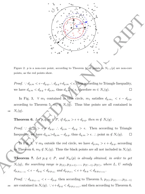
As Fig. 2 shows, l > , the total number of points within the outer black circle is less thanM inP ts, anddo,p< l−, according to Theorem 4, all points
inNl−(p) are non-core points, as the red points within red circle show. Theorem 5. Letp, q, m∈P . Ifdp,m< −dp,q, thenm∈N(q).
ACCEPTED MANUSCRIPT
p o l−ε ε l εFigure 2: pis a non-core point, according to Theorem 4, all points inNl−(p) are non-core
points, as the red points show.
Proof. ∵dp,m< −dp,q,∴dp,q+dp,m< , then according to Triangle Inequality,
we havedq,m< dp,q+dp,m, thusdq,m< , thereforem∈N(q).
In Fig. 3, ∀ m1 contained in blue circle, m1 satisfies dp,m1 < −dp,q,
according to Theorem 5, m1 ∈ N(q). Thus blue points are all contained in N(q).
190
Theorem 6. Letp, q, m ∈P, ifdp,m> +dp,q, thenm /∈N(q).
Proof. ∵ dp,m > + dp,q, ∴ dp,m −dp,q > . Then according to Triangle
Inequality, we have dq,m>dp,m−dp,q, thus dq,m> . ∴point m∈/N(q).
In Fig. 3, ∀ m2 outside the red circle, we have dp,m2 > +dp,q, according
to Theorem 6,m2∈/N(q). Thus the black points are all not included inN(q). Theorem 7. Let p, q ∈ P, and N2(p) is already obtained, in order to get N(q), the searching range is p(L), p(L+1), ..., p(U−1), p(U), where L, U satisfy
dp,p(L−1)< −dp,q< dp,p(L) and dp,p(U) < +dp,q< dp,p(U+1).
Proof. ∵dp,p(L−1) < −dp,q, then according to Theorem 5,p(1), p(2), ..., p(L−1)
are contained inN(q).∵+dp,q< dp,p(U+1), and then according to Theorem 6,
ACCEPTED MANUSCRIPT
Figure 3: Illustration of Theorem 5, Theorem 6 and Theorem 7. All points inN−dp,q(p) (blue points) are inN(q), and black points are all outside the-neighborhood ofq, only red
points are uncertain.
we havep(U+1), p(U+2), ..., p(N)are not contained inN(q). ∴p(L), p(L+1), ..., p(U−1), p(U)
is the searching range for obtainingN(q).
According to Theorem 7, in Fig. 3 the remaining uncertain points (p(L), ..., p(U))
are those red points, which locate in the annular region between blue circle and red circle.
Comprehensively, according to Theorem 5, 6 and 7, in order to obtainN(q),
we only need to search those red points in the annular region. All distance computations frompto blue and black points are reduced.
3.2. The proposed algorithm
We introduce a new clustering algorithm named NQ-DBSCAN based on the
210
theorems mentioned above. Algorithm 3 shows the main procedures of NQ-DBSCAN. Algorithm 4 illustrates the detail of our improved ExpandCluster
which retrieves all density-reachable neighbors from a core point, and Algo-rithm 5 presents the implementation of Theorem 7.
ACCEPTED MANUSCRIPT
Algorithm 3NQ-DBSCAN (P,,MinPts)
Input:
P: a set of unclassified points; : the maximum distance;
MinPts: the minimum points to form a cluster;
Output: cluster id of each point; 1: Initialize cluster idC = 0
2: foreach unclassified pointp∈P do
3: //retrieve all neighbors within 2-neighborhood ofp 4: N2(p)=RangeQuery(p,2)
5: if|N2(p)|> M inP tsthen
6: dists←all distances fromptoN2(p)
7: [distArr, pLoc] =sort(dists) //distArrsaves the sorteddists, whilepLocis a vector that saves the corresponding points such thatdp,pLoc(i)≤dp,pLoc(i+1)
8: if distArr[M inP ts]≤ then
9: // According toTheorem 2pis a core point, then we expand it. 10: drPts=ImprovedExpandCluster(p,pLoc,distArr,,MinPts) 11: Set the cluster id of all points indrPts asC
12: C←C+ 1
13: else
14: Use binary search algorithm findO={o|o∈pLocanddp,o< distArr(M inP ts)−
}, and set all points inOas noise (Theorem 4) 15: end if
16: else
17: SetO={q|q∈N(p)}as noise (Theorem 3)
18: end if
ACCEPTED MANUSCRIPT
In Algorithm 3 (NQ-DBSCAN), the main steps are below.
• Select an unclassified point p from P, then use RangeQuery to retrieve
N2(p) (line 4), and sort the distances formpto its 2-neighbors.
• According to Theorem 2, we can easily judge whether p is core point or not, as shown in line 8.
• If p is a core point, it will use ImprovedExpandCluster to find all points
220
that are density-reachable fromp(drP ts), as shown in line 10. All points
indrP tswill be marked as the same cluster id.
• According to Theorem 3 and Theorem 4, we are able to effectively find non-core points. If | N(p) |< M inP ts, p is a non-core point and its
neighbors are also highly possible to be non-core point, as line 14 shows. If | N2(p)|< M inP ts, then all points in N(p) are labeled as noise, as
line 17 shows.
Algorithm 4 (ImprovedExpandCluster) is a new algorithm that retrieves all density-reachable points, drPts, from point p, which improves Algorithm 2 greatly. The main steps are shown as below.
230
• First initializedrP ts=N(p) by binary searching fromdistArrandpLoc.
• Second, select an unclassified point q from pLoc. If dp,q ≤ we use
NeighborQuery to effectively getN(q), and ifq is a core pointN(q) will
be added to the setdrP ts. Repeat this step until all points in pLocare handled.
• Third, select a new unclassified pointp∈drP ts. Ifpis a core point then use RangeQuery again to update N2(p), pLoc and distArr, and then
repeat the second step, until all points indrP tsare visited.
Algorithm 5 (NeighborQuery) is the implementation of Theorem 7, it uses binary search algorithm to obtain N(q) inN2(p) rather than the whole data 240
ACCEPTED MANUSCRIPT
Algorithm 4ImprovedExpandCluster (p, pLoc, distArr,, MinPts)
Input:
p: reference point;
pLoc: saves all points inN2(p) such thatdp,pLoc(i)≤dp,pLoc(i+1);
distArr: the sorted distances fromptoN2(p);
: the maximum distance;
MinPts: the minimum points to form a cluster.
Output: drPts: all density-reachable neighbor points fromp. 1: binary searchdrP ts={o|o∈pLoc s.t. dp,o≤}
2: foreach pointqsaved inpLocdo
3: ifqis unclassifiedthen
4: if dp,q≤then
5: N(q)=NeighborQuery(p,q,pLoc,distArr,,MinPts)
6: if|N(q)| ≥M inP tsthen 7: drPts=drPts∪N(q) 8: end if 9: end if 10: end if 11: end for
12: p←select an unclassified pointoindrPts 13: if pis a core pointthen
14: N2(p) =RangeQuery(p,2*)
15: dists←distances frompto all points inN2(p)
16: [distArr, pLoc] =sort(dists) 17: go to Line 2
ACCEPTED MANUSCRIPT
Take Fig. 3 for example again, p is a core point, its 2-neighbors have al-ready been retrieved by RangeQuery. ∀q ∈ N(p), in order to retrieve N(q),
NeighborQuery only checks those red points.
Algorithm 5NeighborQuery(p,q,pLoc,distArr,,MinPts)
Input:
p: reference point; q: current search point;
pLoc: the points number of neighbor sequence; distArr: the points distance of neighbor sequence; : the maximum distance;
MinPts: the minimum points to form a cluster;
Output: N(q).
1: // determineLandU according toTheorem 5, 6 and 7
2: binary search index L such thatdistArr(L)> dp,q−
3: binary search index U such thatdistArr(U)< dp,q+
4: possibleN eighbor=pLoc(L:U)
5: N(q)=pLoc(1 :L)S{o|o∈possibleN eighbor s.t. dq,o< }
3.3. Correctness analysis
As shown in Algorithm 4 and 5, based on Theorems 5, 6 and 7 we can see that ifp is a core point Algorithm 4 only retrieve all density-reachable points fromp, which is equivalent to Algorithm 2.
Similarly, based on Theorem 2, 3 and 4, as well as Algorithm 4, NQ-DBSCAN (Algorithm 3) is also guaranteed to be equivalent to NQ-DBSCAN
(Al-250
gorithm 1). Thus NQ-DBSCAN meets the requirement of M aximality and
Conectivity defined in Definition 7, as well as Lemma 1 and Lemma 2 in [33]
are also satisfied.
3.4. Complexity analysis
The key processes in NQ-DBSCAN are RangeQuery and NeighborQuery, and time complexity of NQ-DBSCAN highly depends on them.
The complexity ofRangeQuery can be O(logn) with the help of indexing techniques, such as R*-tree, otherwise isO(n). In this paper, we use
quadtree-ACCEPTED MANUSCRIPT
The complexity of NeighborQuery is O(log(nei)) by using binary search method, whereneiis the number ofp’s neighbors.
Therefore, the whole time complexity of NQ-DBSCAN is O(α∗(log(n) +
nei∗log(nei)) +β∗log(nei)−γ), whereαis execution times ofRangeQuery,β
is execution times ofNeighborQuery, andγis the total number of filtered points that are unnecessary to visit (including some non-core points and noise points), respectively. Obviously,α+β+γ=n, and thenα+β <=n.
In the case ofM inP tsis very large such that γ→n, i.e. most points are identified as non-core points directly, the complexity is O(1). However, it is
270
meaningless. The best complexity is O(n), in the case of both α and nei are small, whileβ→n. Generally, the average complexity of NQ-DBSCAN is about
O(n∗log(n)) ifandM inP tsare properly chosen. Of course, without indexing technique, the average complexity is alsoO(n2).
4. Experiments
In this section, we conduct experiments to evaluate the performance of NQ-DBSCAN, and make comparisons with original DBSCAN and ρ-approximate DBSCAN [40], on synthetic and realtime data sets.
4.1. Algorithms
Algorithms. Our experiments involve four algorithms as follows:
280
• DBSCAN: the original DBSCAN algorithm in [33];
• NQ-DBSCAN: the proposed algorithm without using indexing technique;
• “NQ-DBSCAN with indexing”: the proposed algorithm with quadtree-like hierarchical tree grid indexing;
ACCEPTED MANUSCRIPT
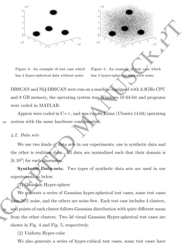
Figure 4: An example of test case which has 4 hyper-spherical data without noise.
Figure 5: An example of test case which has 4 hyper-spherical data with noise.
DBSCAN and NQ-DBSCAN were run on a machine equipped with 3.3GHz CPU and 8 GB memory, the operating system was Windows 10 64-bit and programs were coded in MATLAB.
Approx were coded in C++, and was run on Linux (Ubuntu 14.04) operating system with the same hardware configuration.
290
4.2. Data sets
We use two kinds of data sets in our experiments, one is synthetic data and the other is realtime data. All data are normalized such that their domain is [0,105] for each dimension.
Synthetic Data sets. Two types of synthetic data sets are used in our experiments as below.
(1) Gaussian Hyper-sphere
We generate a series of Gaussian hyper-spherical test cases, some test cases have 20% noise, and the others are noise-free. Each test case includes 4 clusters, and points of each cluster follows Gaussian distribution with quite different mean
300
from the other clusters. Two 3dvisual Gaussian Hyper-spherical test cases are shown in Fig. 4 and Fig. 5, respectively.
(2) Uniform Hyper-cube
ACCEPTED MANUSCRIPT
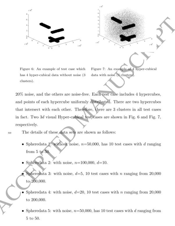
Figure 6: An example of test case which has 4 hyper-cubical data without noise (3 clusters).
Figure 7: An example of 4 hyper-cubical data with noise (3 clusters).
20% noise, and the others are noise-free. Each test case includes 4 hypercubes, and points of each hypercube uniformly distributed. There are two hypercubes that intersect with each other. Therefore, there are 3 clusters in all test cases in fact. Two 3dvisual Hyper-cubical test cases are shown in Fig. 6 and Fig. 7, respectively.
The details of these data sets are shown as follows:
310
• Spheredata 1: without noise,n=50,000, has 10 test cases withdranging from 5 to 50.
• Spheredata 2: with noise, n=100,000,d=10.
• Spheredata 3: with noise,d=5, 10 test cases with nranging from 20,000 to 200,000.
• Spheredata 4: with noise,d=20, 10 test cases withnranging from 20,000 to 200,000.
• Spheredata 5: with noise,n=50,000, has 10 test cases withdranging from 5 to 50.
ACCEPTED MANUSCRIPT
• Spheredata 6: with noise, n=100,000, has 10 test cases with d ranging
320
from 5 to 50.
• Cubedata 1: without noise, n=50,000, has 10 test cases withd ranging from 5 to 50.
• Cubedata 2: with noise,d=5, has 10 test cases withnranging from 10,000 to 100,000.
• Cubedata 3: with noise, d=10, has 10 test cases with n ranging from 10,000 to 100,000.
• Cubedata 4: with noise,n=50,000, has 15 test cases withdranging from 10 to 150.
Real Data sets. Some real data sets were employed in our experiments as
330
follows:
The first, House (household) is a 7 dimensional data set with cardinality 2,075,259, which includes all the attributes of the Household database comes from the UCI archive2except the temporal columns date and time. Points in
the original database with missing coordinates were removed.
The second, ReactionNetwork is KEGG Metabolic Reaction Network (Undi-rected) Data Set which also comes from UCI. It is a 28-dimensional data set with cardinality 65,554.
The third, BlogFeedback [55] also comes from the UCI archive. It is a 59-dimensional data set with cardinality 52,397 obtained by taking the first 59
340
numeric attributes and the 60th-280th attributes are omitted, because most
values in the 60th-280th attributes are zero.
The fourth, KDD04 is KDD Cup 2004 data. It is 76-dimensional data set with cardinality 145,751.
The fifth, MNIST3 is a handwritten digits data set, which includes 70,000
2http://archive.ics.uci.edu/ml 3http://yann.lecun.com/exdb/mnist/
ACCEPTED MANUSCRIPT
cardinality 10,000.
The sixth, PAM (PAMPA2), which comes from UCI, is a 4-dimensional data
350
set with cardinality 3,850,505.
The last one is MORPH [56] which is the largest publicly available longi-tudinal face database4, includes 79,897 face photographs with size of 70×80
pixel. Also, we pick up 10,000 face photographs of MORPH in our experiments. We convert the RGB images to gray images, and then transform each gray im-age matrix into a feature vector with 70×80 = 5,600 dimensions. Therefore, MORPH used in our experiments is a 5600-dimensional data set with cardinality 10,000.
4.3. Experiment 1: Two Examples
We benchmark NQ-DBSCAN on two test cases, the first one is t4.8k [57],
360
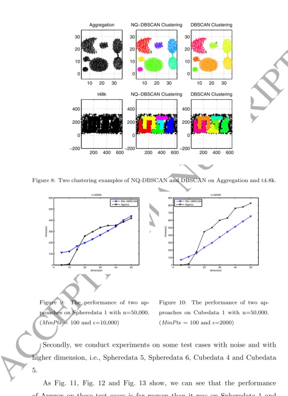
which is a 2-dimensional data set with cardinality 8,000, and the other is Ag-gregation [58], which is a 2-dimensional data set with cardinality 788. The dis-tribution of two data sets and the clusters obtained by NQ-DBSCAN are shown in Fig. 8. It illustrates that NQ-DBSCAN has the same ability as DBSCAN to detect complex shapes.
4.4. Experiment 2: Influence of Noise and Dimensionality
The purpose of this part is to check impaction of noise and dimensionality on NQ-DBSCAN and Approx.
Firstly, we conduct an experiment on Spheredata 1 and Cubedata 1 which are noise-free. As shown in Fig. 9 and Fig. 10, we can see that in the case of
370
dimension is less than 50, Approx and NQ-DBSCAN performs similarly on both test cases, and the running time increase linearly with dimension.
ACCEPTED MANUSCRIPT
10 20 30 0 10 20 30 Aggregation 10 20 30 0 10 20 30 NQ−DBSCAN Clustering 10 20 30 0 10 20 30 DBSCAN Clustering 200 400 600 −200 0 200 400 t48k 200 400 600 −200 0 200 400 NQ−DBSCAN Clustering 200 400 600 −200 0 200 400 DBSCAN ClusteringFigure 8: Two clustering examples of NQ-DBSCAN and DBSCAN on Aggregation and t4.8k.
0 10 20 30 40 50 0 100 200 300 400 500 600 dimension time(sec) n=50000 NQ−DBSCAN Approx
Figure 9: The performance of two ap-proaches on Spheredata 1 with n=50,000. (MinPts= 100 and=10,000) 0 10 20 30 40 50 0 100 200 300 400 500 600 700 800 900 dimension time(sec) n=50000 NQ−DBSCAN Approx
Figure 10: The performance of two ap-proaches on Cubedata 1 with n=50,000. (MinPts= 100 and=2000)
Secondly, we conduct experiments on some test cases with noise and with higher dimension, i.e., Spheredata 5, Spheredata 6, Cubedata 4 and Cubedata 5.
As Fig. 11, Fig. 12 and Fig. 13 show, we can see that the performance of Approx on these test cases is far worsen than it was on Spheredata 1 and
ACCEPTED MANUSCRIPT
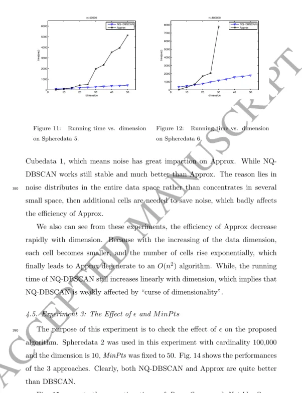
0 10 20 30 40 50 0 1000 2000 3000 dimension time(sec)Figure 11: Running time vs. dimension on Spheredata 5. 0 10 20 30 40 50 0 1000 2000 3000 4000 dimension time(sec)
Figure 12: Running time vs. dimension on Spheredata 6.
Cubedata 1, which means noise has great impaction on Approx. While NQ-DBSCAN works still stable and much better than Approx. The reason lies in noise distributes in the entire data space rather than concentrates in several
380
small space, then additional cells are needed to save noise, which badly affects the efficiency of Approx.
We also can see from these experiments, the efficiency of Approx decrease rapidly with dimension. Because with the increasing of the data dimension, each cell becomes smaller, and the number of cells rise exponentially, which finally leads to Approx degenerate to an O(n2) algorithm. While, the running
time of NQ-DBSCAN still increases linearly with dimension, which implies that NQ-DBSCAN is weakly affected by “curse of dimensionality”.
4.5. Experiment 3: The Effect ofand M inP ts
The purpose of this experiment is to check the effect of on the proposed
390
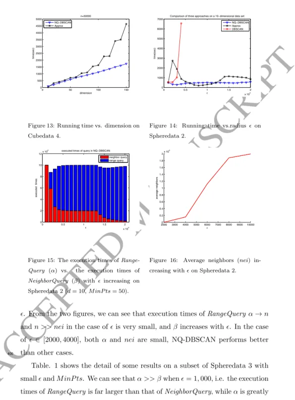
algorithm. Spheredata 2 was used in this experiment with cardinality 100,000 and the dimension is 10,MinPtswas fixed to 50. Fig. 14 shows the performances of the 3 approaches. Clearly, both NQ-DBSCAN and Approx are quite better than DBSCAN.
Fig. 15 presents the execution times of RangeQuery and NeighborQuery, and Fig. 16 plots the average neighbors found in RangeQuery increasing with
ACCEPTED MANUSCRIPT
0 50 100 150 0 500 1000 1500 2000 2500 3000 3500 4000 4500 5000 dimension time(sec) n=50000 NQ−DBSCAN ApproxFigure 13: Running time vs. dimension on Cubedata 4. 0 0.5 1 1.5 2 x 10⁴ 0 1000 2000 3000 4000 5000 6000 7000 ε time(sec)
Comparison of three approaches on a 10−dimensional data set NQ−DBSCAN Approx DBSCAN
Figure 14: Running time vs.radius on Spheredata 2. 0 0.5 1 1.5 2 x 10⁴ 0 2 4 6 8 10 12x 10 4 ε executed times
executed times of query in NQ−DBSCAN neighbor query range query
Figure 15: The execution times of Range-Query (α) vs. the execution times of NeighborQuery (β) with increasing on Spheredata 2 (d= 10,M inP ts= 50). 20000 3000 4000 5000 6000 7000 8000 9000 10000 0.2 0.4 0.6 0.8 1 1.2 1.4 1.6 1.8 2x 10 4 average neighbors ε
Figure 16: Average neighbors (nei) in-creasing withon Spheredata 2.
. From the two figures, we can see that execution times ofRangeQuery α→n
andn >> neiin the case ofis very small, andβ increases with. In the case of ∈ [2000,4000], both α and nei are small, NQ-DBSCAN performs better than other cases.
400
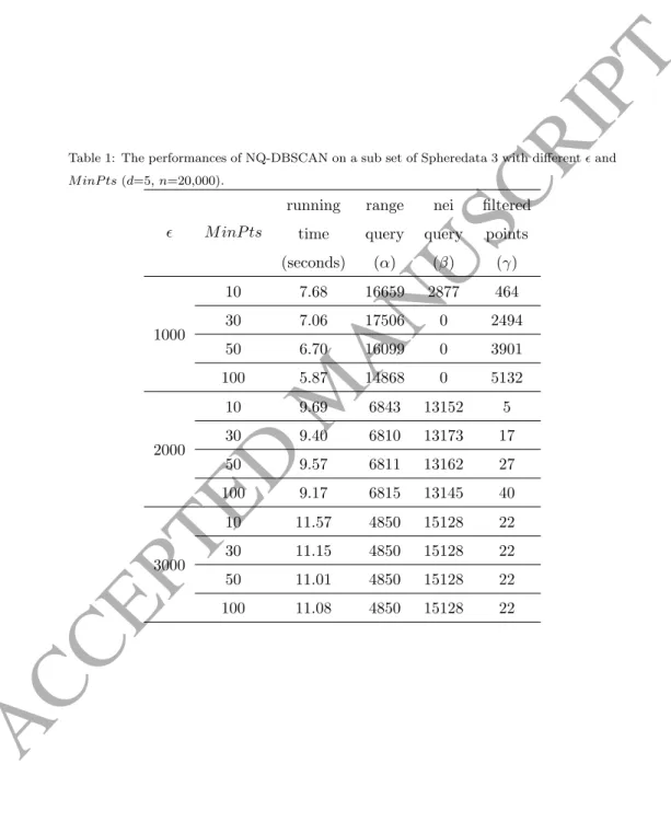
Table. 1 shows the detail of some results on a subset of Spheredata 3 with smallandM inP ts. We can see thatα >> βwhen= 1,000, i.e. the execution times ofRangeQueryis far larger than that ofNeighborQuery, whileαis greatly reduced when= 2,000 and = 3,000. We also notice that the running time
ACCEPTED MANUSCRIPT
Table 1: The performances of NQ-DBSCAN on a sub set of Spheredata 3 with differentand M inP ts(d=5,n=20,000). M inP ts running time (seconds) range query (α) nei query (β) filtered points (γ) 1000 10 7.68 16659 2877 464 30 7.06 17506 0 2494 50 6.70 16099 0 3901 100 5.87 14868 0 5132 2000 10 9.69 6843 13152 5 30 9.40 6810 13173 17 50 9.57 6811 13162 27 100 9.17 6815 13145 40 3000 10 11.57 4850 15128 22 30 11.15 4850 15128 22 50 11.01 4850 15128 22 100 11.08 4850 15128 22
ACCEPTED MANUSCRIPT
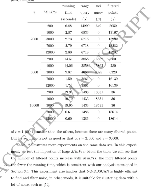
Table 2: The performances of NQ-DBSCAN on a sub set of Spheredata 3 with largeM inP ts (d=5,n=20,000). M inP ts running time (seconds) range query (α) nei query (β) filtered points (γ) 2000 200 6.88 14299 649 5052 1000 2.87 6833 0 13167 3000 2.73 6718 0 13282 7000 2.79 6718 0 13282 12000 2.80 6718 0 13282 5000 200 14.51 3858 15862 280 1000 14.06 3858 15862 280 3000 9.87 4655 9025 6320 7000 1.59 3861 0 16139 12000 1.74 3861 0 16139 10000 200 19.91 1433 18531 36 1000 19.79 1433 18531 36 3000 19.95 1433 18531 36 7000 0.61 1386 0 18614 12000 0.60 1386 0 18614
of= 1,000 is smaller than the others, because there are many filtered points. But its accuracy is not as good as that of= 2,000 and= 3,000.
Table. 2 illustrates more experiments on the same data set. In this experi-ment, we test the impaction of largeM inP ts. From the table we can see that the number of filtered points increase with M inP ts, the more filtered points the fewer the running time, which is consistent with our analysis mentioned in
410
Section 3.4. This experiment also implies that NQ-DBSCAN is highly efficient to find and filter noise, in other words, it is suitable for clustering data with a lot of noise, such as [59].
ACCEPTED MANUSCRIPT
DBSCAN, “NQ-DBSCAN with indexing” and Approx by changing the cardi-nalities of these cases.
Because Approx runs linearly in low-dimension, we can see that Approx outperforms NQ-DBSCAN in Fig. 17 and Fig. 18. However, with dimension
420
increasing, things go different. In Fig. 19, we can see that in this 10-dimensional data set, Approx is still better than NQ-DBSCAN and “NQ-DBSCAN with indexing”, but their performances are closer than that in 5 dimension. And then, Fig. 20 shows that the performance of Approx is inferior to both NQ-DBSCAN and “NQ-NQ-DBSCAN with indexing” in the 20-dimensional data set (Spheredata 4).
All experiments above obtain correct results as we expected, i.e. in Fig. 17 and Fig. 19, we obtain 4 hyper-spherical clusters, and in Fig. 18 and Fig. 20, we get 3 clusters which include 4 hyper-cubes.
We also can see that “NQ-DBSCAN with indexing” seems to be an O(n)
430
algorithm, because properandM inP tsare used such thatαandneiare both small and β →n, which is consistent with the theoretical analysis mentioned above.
4.7. Experiment 5: Experiments on Realtime Applications
In order to test the performance of NQ-DBSCAN and “NQ-DBSCAN with indexing” in realtime applications, we benchmark it on six test cases with differ-ent dimensions, i.e. Household (7 dim), ReactionNetwork (28 dim) , BlogFeed-back (59 dim), KDD04 (76 dim), MNIST (784 dim) andMORPH (5,600 dim), and compare them withρ-Approximate DBSCAN. In the following experiments,
MinPts are all fixed to 100.
440
Fig. 21 and Fig. 22 show that Approx runs linearly in Household (7 dim) and ReactionNetwork (28 dim), and its performance is better than the proposed
ACCEPTED MANUSCRIPT
0.2 0.4 0.6 0.8 1 1.2 1.4 1.6 1.8 2 x 10⁴ 0 200 400 600 800 1000 1200 1400 1600 1800 time(sec) n NQ−DBSCAN NQ−DBSCAN with indexing ApproxFigure 17: Running time vs. cardinal-ity on Spheredata 3 (5 dim,=2,000 and MinPts=100). 0.5 1 1.5 2 2.5 3 3.5 4 4.5 5 x 10⁴ 0 50 100 150 200 250 300 time(sec) n NQ−DBSCAN NQ−DBSCAN with indexing Approx
Figure 18: Running time vs. cardinal-ity n on Cubedata 2 (5 dim,=2000 and MinPts=100). 0.5 1 1.5 2 2.5 3 3.5 4 4.5 5 x 10⁴ 0 50 100 150 200 250 300 350 400 450 500 time(sec) n NQ−DBSCAN NQ−DBSCAN with indexing Approx
Figure 19: Running time vs. cardinality n on Cubedata 3 (10 dim, =2000 and MinPts=100). 2 4 6 8 10 12 14 16 x 104 0 500 1000 1500 2000 2500 3000 3500 4000 4500 5000 time(sec) n NQ−DBSCAN Approx NQ−DBSCAN with indexing
Figure 20: Running time vs. cardinality on Spheredata 4. (20 dim, =2,000 and MinPts=100)
algorithm (One reason that the proposed algorithm runs slower in ReactionNet-work is the code efficiency in Matlab is not as good as C++).
While the comparisons in Fig. 23 and Fig. 24 present that Approx runs in
O(n2), which is clearly inferior to “NQ-DBSCAN with indexing” on
BlogFeed-back (59-dim) and KDD04 (76 dim), respectively.
Clearly, we can see that the higher the dimension, the more advantages the proposed algorithm to Approx, and the four figures above prove that “NQ-DBSCAN with indexing” runs inO(n∗log(n)).
ACCEPTED MANUSCRIPT
0.4 0.6 0.8 1 1.2 1.4 1.6 1.8 2 x 10⁶ 0 500 1000 1500 2000 time(sec) nFigure 21: Running time VS Cardinality on HouseHold (7 dim) with= 1,000 .
1 2 3 4 5 6 7 x 10⁴ 0 50 100 150 time(sec) n
Figure 22: Running time VS Cardi-nality on ReactionNetwork (28 dim) with = 1,000 . 0.5 1 1.5 2 2.5 3 3.5 4 4.5 5 x 10⁴ 0 50 100 150 200 250 time(sec) n Approx NQ−DBSCAN NQ−DBSCAN with indexing
Figure 23: Running time VS Cardinality on BlogFeedback (59 dim) with= 1,000.
2 3 4 5 6 7 8 9 10 11 x 104 0 200 400 600 800 1000 1200 1400 1600 1800 2000 time(sec) n Approx NQ−DBSCAN with indexing
Figure 24: Running time VS Cardinality on KDD04 (76 dim) with= 1,000.
The following two experiments are conducted on MNIST andMORPH are that very high-dimensional and sparse, the quadtree-like hierarchical tree grid fails to work. Thus, we only compare NQ-DBSCAN and Approx by changing different. We can see NQ-DBSCAN outperforms Approx as Fig. 25 and Fig. 26 illustrate. The reason lies in the grid technique is useless in high dimension as mentioned in Theorem 1. While NQ-DBSCAN seems free from dimensionality, which makes it more suitable for clustering realtime data than Approx.
ACCEPTED MANUSCRIPT
0 500 1000 1500 2000 2500 3000 0 500 1000 1500 2000 2500 3000 3500 4000 4500 5000 ε time(sec) Experiments on MNIST NQ−DBSCAN ApproxFigure 25: The performance of two ap-proaches on MNIST (784 dim).
20000 2500 3000 3500 4000 4500 5000 5500 1000 2000 3000 4000 5000 6000 7000 8000 9000 ε time(sec) Experiments on MORPH NQ−DBSCAN Approx
Figure 26: The performance of two ap-proaches on MORPH (5,600 dim).
4.8. The robust of algorithm
According to Huber[60], a robust procedure can be characterized by the following: 1) it should have a reasonably good efficiency (accuracy) at the
as-460
sumed model; 2) small deviations from the model assumptions should impair the performance only by a small amount; and 3) larger deviations from the model assumptions should not cause a catastrophe.
In order to test the accuracy of the proposed algorithm andρ-approximate DBSCAN, we conduct some experiments based on an assumption that the clus-tering labels obtained by DBSCAN is the standard correct result, and evaluate the precision of two approaches as following, which is also used in our previous works[61, 62].
Firstly, we use the original DBSCAN to cluster a data set, and return cluster labels L1 ={A1, A2, ..., Ak}. Secondly, run NQ-DBSCAN and ρ-approximate 470
DBSCAN on the same data set, and obtainL2 = {B1, B2, ..., Bm} and L3 =
{C1, C2, ..., Cp}, respectively.
As we know, the clustering results got by a clustering algorithm may have different labels from that got by the other algorithm, e.g. cluster ‘A1’ obtained by one approach may be the same as cluster ‘B2’ of the other. Therefore, we have to match labels first, then use the matched labels to calculatePrecision. In our experiments, we use Kuhn-Munkras[63] to maximum match two cluster
ACCEPTED MANUSCRIPT
data set BLOG [2000,30] HOUSE [500,30] PAM [500,30] Approx 94.54% 99.67% 99.78% NQ-DBSCAN 99.97% 99.6% 100%
labels, which has been used in our previous works [61, 62].
For example, if a data set has 3 clusters labeled as ‘A1’, ‘A2’ and ‘A3’ obtained by DBSCAN, and our method finds 4 clusters with labels ‘B1’, ‘B2’,
480
‘B3’ and ‘B4’ on the same data set. Suppose there are 3 matched pairs found by Kuhn-Munkres algorithm: (‘A1’,‘B2’), (‘A2’, ‘B1’) and (‘A3’, ‘B4’). If p is labeled as ‘A1’ by DBSCAN and clustered as ‘B2’ by our approach, respectively, we consider this prediction as correct. If p is labeled as ‘A1’ by DBSCAN and clustered as ‘B1’ by our approach it is wrong. Similar to other cases.
As presented in Table. 3, the precisions truly speak of that our approach nearly achieves the same results as DBSCAN, the petty difference is caused by the visiting order is different from that of original DBSCAN, because DBSCAN is non-determinative. While ρ-approximate DBSCAN is little inferior to NQ-DBSCAN.
490
In order to evaluate the performance of NQ-DBSCAN on data sets with deviations, we select 10% data points from BLOG, HOU SE and P AM, re-spectively, and then shift these points randomly in each dimension by adding a random valueη, whereη=of f set∗random(), andof f setis predefined. As Ta-ble. 4 demonstrates, the accuracies of both NQ-DBSCAN andρ-Approximate DBSCAN are similarly affected by the deviations of data set, but it is accept-able.
4.9. Comprehensive Analysis
From all experiments above, we can see that Approx runs linearly in low dimension. However, with the increasing of dimension Approx degenerates to
ACCEPTED MANUSCRIPT
Table 4: The precision of NQ-DBSCAN on three data sets with deviations. All accuracies are calculated by comparing to the result of original DBSCAN. The parameters of NQ-DBSCAN are given in the formation as [, MinPts].
offset BLOG [2000,30] HOUSE[500,30] PAM[500,30]
NQ-DBSCAN 100 99.92% 99.31% 99.78% 200 99.66% 99.73% 99.77% 300 90.29% 89.93% 99.74% 400 90.29% 89.93% 98.76% 500 90.29% 89.93% 93.63% Approx 100 94.49% 99.65% 99.78% 200 94.30% 99.38% 99.77% 300 92.77% 89.79% 99.68% 400 85.92% 89.79% 98.98% 500 85.92% 89.79% 93.68%
be anO(n2) algorithm. While “NQ-DBSCAN with indexing” averagely runs in
O(n) orO(n∗log(n)) in many cases.
In very large high dimension NQ-DBSCAN still outperforms Approx without indexing technique. The reason lies in the grid techniques used in Approx is useless in high dimension, while the neighbor searching technique used in NQ-DBSCAN is almost not affected by the dimensionality.
In the case of data sets having a lot of noise, NQ-DBSCAN works much better, because noise has side effects on Approx. The underlying cause is that noise always distributes in the whole data space rather than concentrates in some small regions, which results in many cells are needed to save noise, and then
510
leads to the efficiency ofρ-approximate rapidly decline. Due to the capability of effectively finding non-core points (Theorem 3 and 4), NQ-DBSCAN can run inO(n) expected time.
In addition, NQ-DBSCAN is an exact algorithm, which is also an important advantage to the approximate algorithmρ-Approximate DBSCAN.
ACCEPTED MANUSCRIPT
and most of these data are high dimensional with a lot of noise, which bring great challenging to clustering. DBSCAN is a creative and elegant technique for density-based clustering. However, it is rendered almost useless for
high-520
dimensional data, due to the “curse of dimensionality”, which limits its applica-bility in many realtime applications. ρ-approximate DBSCAN [40] is an efficient approach designed to replace DBSCAN for big data. By using quadtree-like hier-archical grid and small sacrifice in accuracy,ρ-approximate has a computational time that scales only linearly inn. However, it declines to anO(n2) algorithm
in high dimension because the grid technique is also useless in high dimension. Also, we find the efficiency of ρ-approximate is greatly reduced when dealing with high dimensional data that has much noise, because the grid technique is useless in high dimension and noise needs additional cells to save.
In this paper, we propose a clustering algorithm, named NQ-DBSCAN which
530
may return the exact result as DBSCAN, to improve DBSCAN, by using neigh-bor searching technique and indexing technique to filter great number of un-necessary density computations. The underlying idea is: point p and point q
should have similar neighbors, providedpandq are close to each other; given a certain, the closer they are, the more similar their neighbors are.
Our experiments have shown that the proposed method outperforms ρ -approximate in high dimension, also it performs better in data sets with a lot of noise. Although, the worse complexity of NQ-DBSCAN is stillO(n2), but its
average complexity is aboutO(n∗log(n)) with the help of indexing technique, and the best case isO(n) if proper parameters (andM inP ts) are used.
540
The indexing technique we used is quadtree-like hierarchical tree grid, but it fails to work in some sparse and very high-dimensional data. Therefore, in future work, we will try to improve quadtree-like hierarchical tree grid, by combining the merits of other techniques, such as product quantization for nearest neighbor search [52], LSH (Locality-Sensitive Hashing) [53], FLANN [54] etc.
ACCEPTED MANUSCRIPT
Acknowledgment
The National Science Foundation of China (No.61673186,71771094) ; this work was supported by the Open Project Program of the National Laboratory of Pattern Recognition (NLPR) (NO.201700002); the Open Project Program of the State Key Lab of CAD&CG(Grant No.A1722), Zhejiang University; the
550
Natural Science Foundation of Fujian Province (No.2016J01303); Project of science and technology plan of Fujian Province of China (No.2017H01010065); the Graduate Students Research and Innovation Ability Cultivation Plan of Huaqiao University (No.1511414009); the Huaqiao University graduate research project of education reform (16YJG13).
Reference References
[1] J. Song, L. Gao, F. Nie, H. T. Shen, Y. Yan, N. Sebe, Optimized graph learning using partial tags and multiple features for image and video anno-tation, IEEE Transactions on Image Processing 25 (11) (2016) 4999–5011.
560
[2] J. Song, L. Gao, F. Zou, Y. Yan, N. Sebe, Deep and fast: Deep learning hashing with semi-supervised graph construction, Image and Vision Com-puting.
[3] J. Song, H. T. Shen, J. Wang, Z. Huang, N. Sebe, J. Wang, A distance-computation-free search scheme for binary code databases, IEEE Transac-tions on Multimedia 18 (3) (2016) 484–495.
[4] W. Zhou, M. Yang, X. Wang, H. Li, Y. Lin, Q. Tian, Scalable feature matching by dual cascaded scalar quantization for image retrieval, IEEE transactions on pattern analysis and machine intelligence 38 (1) (2016) 159–171.
ACCEPTED MANUSCRIPT
[6] A. K. Rajagopal, R. Subramanian, E. Ricci, R. L. Vieriu, O. Lanz, N. Sebe, et al., Exploring transfer learning approaches for head pose classification from multi-view surveillance images, International Journal of Computer Vision 109 (1-2) (2014) 146–167.
[7] Y. Yan, E. Ricci, R. Subramanian, G. Liu, O. Lanz, N. Sebe, A multi-task learning framework for head pose estimation under target motion, IEEE transactions on pattern analysis and machine intelligence 38 (6) (2016)
580
1070–1083.
[8] B. F. Qaqish, J. J. OBrien, J. C. Hibbard, K. J. Clowers, Accelerating high dimensional clustering with lossless data reduction, Bioinformatics (2017) btx328.
[9] Z. Deng, K.-S. Choi, Y. Jiang, J. Wang, S. Wang, A survey on soft subspace clustering, Information Sciences 348 (2016) 84–106.
[10] O. Limwattanapibool, S. Arch-int, Determination of the appropriate pa-rameters for k-means clustering using selection of region clusters based on density dbscan (srcd-dbscan), Expert Systems.
[11] L. Bai, X. Cheng, J. Liang, H. Shen, Y. Guo, Fast density clustering
strate-590
gies based on the k-means algorithm, Pattern Recognition 71 (2017) 375– 386.
[12] N. A. Yousri, M. S. Kamel, M. A. Ismail, A distance-relatedness dynamic model for clustering high dimensional data of arbitrary shapes and densi-ties, Pattern Recognition 42 (7) (2009) 1193–1209.
[13] C. Zhong, D. Miao, R. Wang, A graph-theoretical clustering method based on two rounds of minimum spanning trees, Pattern Recognition 43 (3) (2010) 752–766.
ACCEPTED MANUSCRIPT
[14] M. Ester, H.-P. Kriegel, J. Sander, Algorithms and applications for spatial data mining, Geographic Data Mining and Knowledge Discovery 5 (6).
600
[15] W. A. Barbakh, Y. Wu, C. Fyfe, Non-standard parameter adaptation for exploratory data analysis, Vol. 249, Springer, 2009.
[16] J. Han, J. Pei, M. Kamber, Data mining: concepts and techniques, Elsevier, 2011.
[17] J. Hou, W. Liu, E. Xu, H. Cui, Towards parameter-independent data clus-tering and image segmentation, Pattern Recognition 60 (2016) 25–36.
[18] S. Mitra, P. P. Kundu, Satellite image segmentation with shadowed c -means, Information Sciences 181 (17) (2011) 3601–3613.
[19] S. Das, S. Sil, Kernel-induced fuzzy clustering of image pixels with an improved differential evolution algorithm, Information Sciences An
Inter-610
national Journal 180 (8) (2010) 1237–1256.
[20] Y. C. Song, H. D. Meng, M. J. OGrady, G. M. P. OHare, The applica-tion of cluster analysis in geophysical data interpretaapplica-tion, Computaapplica-tional Geosciences 14 (2) (2010) 263–271.
[21] A. Ghosh, N. S. Mishra, S. Ghosh, Fuzzy clustering algorithms for unsu-pervised change detection in remote sensing images, Information Sciences 181 (4) (2011) 699–715.
[22] Y. J. Wang, H. S. Lee, A clustering method to identify representative fi-nancial ratios, Information Sciences 178 (4) (2008) 1087–1097.
[23] J. Li, K. Wang, L. Xu, Chameleon based on clustering feature tree and
620
its application in customer segmentation, Annals of Operations Research 168 (1) (2009) 225–245.
[24] Q. Bsoul, J. Salim, L. Q. Zakaria, An intelligent document clustering ap-proach to detect crime patterns , Procedia Technology 11 (1) (2013) 1181– 1187.
ACCEPTED MANUSCRIPT
[26] V. P. Ananthi, P. Balasubramaniam, T. Kalaiselvi, A new fuzzy clustering algorithm for the segmentation of brain tumor, Soft Computing (2015) 1–
630
21.
[27] R. Chinchuluun, W. S. Lee, J. Bhorania, P. M. Pardalos, Clustering and Classification Algorithms in Food and Agricultural Applications: A Survey, Springer US, 2009.
[28] A. Hatamlou, Black hole: A new heuristic optimization approach for data clustering, Information Sciences 222 (3) (2013) 175–184.
[29] J. G. Lee, J. Han, K. Y. Whang, Trajectory clustering: a partition-and-group framework, in: ACM SIGMOD International Conference on Man-agement of Data, 2007, pp. 593–604.
[30] X. T. Yuan, B. G. Hu, R. He, Agglomerative mean-shift clustering, IEEE
640
Transactions on Knowledge and Data Engineering 24 (2) (2012) 209–219.
[31] W.-Y. Chen, Y. Song, H. Bai, C.-J. Lin, E. Y. Chang, Parallel spectral clustering in distributed systems, IEEE transactions on pattern analysis and machine intelligence 33 (3) (2011) 568–586.
[32] S. Mitra, A parallel clustering technique for the vehicle routing problem with split deliveries and pickups, Journal of the Operational Research So-ciety 59 (11) (2008) 1532–1546.
[33] M. Ester, H.-P. Kriegel, J. Sander, X. Xu, A density-based algorithm for discovering clusters in large spatial databases with noise., in: Kdd, Vol. 96, 1996, pp. 226–231.
650
[34] B. Borah, D. Bhattacharyya, An improved sampling-based dbscan for large spatial databases, in: Intelligent Sensing and Information Processing, 2004. Proceedings of International Conference on, IEEE, 2004, pp. 92–96.
ACCEPTED MANUSCRIPT
[35] C. Ruiz, M. Spiliopoulou, E. Menasalvas, C-dbscan: Density-based clus-tering with constraints, in: International Workshop on Rough Sets, Fuzzy Sets, Data Mining, and Granular-Soft Computing, Springer, 2007, pp. 216– 223.
[36] Y. He, H. Tan, W. Luo, H. Mao, D. Ma, S. Feng, J. Fan, Mr-dbscan: an efficient parallel density-based clustering algorithm using mapreduce, in: Parallel and Distributed Systems (ICPADS), 2011 IEEE 17th International
660
Conference on, IEEE, 2011, pp. 473–480.
[37] K. M. Kumar, A. R. M. Reddy, A fast dbscan clustering algorithm by accelerating neighbor searching using groups method, Pattern Recognition 58 (2016) 39–48.
[38] A. Tramacere, C. Vecchio, γ-ray dbscan: a clustering algorithm applied to fermi-lat γ-ray data-i. detection performances with real and simulated data, Astronomy & Astrophysics 549 (2013) A138.
[39] S. T. Mai, S. Goebl, C. Plant, A similarity model and segmentation al-gorithm for white matter fiber tracts, in: 2012 IEEE 12th International Conference on Data Mining, IEEE, 2012, pp. 1014–1019.
670
[40] J. Gan, Y. Tao, Dbscan revisited: Mis-claim, un-fixability, and approxima-tion, in: Proceedings of the 2015 ACM SIGMOD International Conference on Management of Data, ACM, 2015, pp. 519–530.
[41] J. Wang, Z. Deng, K.-S. Choi, Y. Jiang, X. Luo, F.-L. Chung, S. Wang, Distance metric learning for soft subspace clustering in composite kernel space, Pattern Recognition 52 (2016) 113–134.
[42] P. Qian, Y. Jiang, Z. Deng, L. Hu, S. Sun, S. Wang, R. F. Muzic, Cluster prototypes and fuzzy memberships jointly leveraged cross-domain maxi-mum entropy clustering, IEEE transactions on cybernetics 46 (1) (2016) 181–193.
ACCEPTED MANUSCRIPT
[44] Z. Deng, K.-S. Choi, F.-L. Chung, S. Wang, Enhanced soft subspace clus-tering integrating within-cluster and between-cluster information, Pattern Recognition 43 (3) (2010) 767–781.
[45] A. Gunawan, A faster algorithm for dbscan, Ph.D. thesis, Masters thesis, Technische University Eindhoven (2013).
[46] P. Viswanath, V. S. Babu, Rough-dbscan: A fast hybrid density based clustering method for large data sets, Pattern Recognition Letters 30 (16)
690
(2009) 1477–1488.
[47] D. Birant, A. Kut, St-dbscan: An algorithm for clustering spatial–temporal data, Data & Knowledge Engineering 60 (1) (2007) 208–221.
[48] S. Mahran, K. Mahar, Using grid for accelerating density-based clustering, in: IEEE International Conference on Computer and Information Technol-ogy, 2008, pp. 35–40.
[49] C. Xiaoyun, M. Yufang, Z. Yan, W. Ping, Gmdbscan: Multi-density dbscan cluster based on grid, in: IEEE International Conference on E-Business Engineering, 2008, pp. 780–783.
[50] O. Uncu, W. A. Gruver, D. B. Kotak, D. Sabaz, Gridbscan: Grid
density-700
based spatial clustering of applications with noise, in: IEEE International Conference on Systems, Man and Cybernetics, 2006, pp. 2976–2981.
[51] L. Zhang, Z. Xu, F. Si, Gcmddbscan: Multi-density dbscan based on grid and contribution, in: IEEE International Conference on Dependable, Au-tonomic and Secure Computing, 2013, pp. 502–507.
[52] H. Jegou, M. Douze, C. Schmid, Product quantization for nearest neighbor search, IEEE transactions on pattern analysis and machine intelligence 33 (1) (2011) 117–128.
ACCEPTED MANUSCRIPT
[53] A. Andoni, P. Indyk, Near-optimal hashing algorithms for approximate nearest neighbor in high dimensions, Commun. ACM 51 (1) (2008)
710
117C122.
[54] D. G. L. Marius Muja, Scalable nearest neighbor algorithms for high dimen-sional data, IEEE transactions on pattern analysis and machine intelligence 36 (11) (2014) 2227–2240.
[55] K. Buza, Feedback prediction for blogs, in: Data analysis, machine learning and knowledge discovery, Springer, 2014, pp. 145–152.
[56] K. Ricanek, T. Tesafaye, Morph: a longitudinal image database of normal adult age-progression, in: International Conference on Automatic Face and Gesture Recognition, 2006, pp. 341–345.
[57] G. Karypis, E.-H. Han, V. Kumar, Chameleon: Hierarchical clustering
720
using dynamic modeling, Computer 32 (8) (1999) 68–75.
[58] A. Gionis, H. Mannila, P. Tsaparas, Clustering aggregation, ACM Trans-actions on Knowledge Discovery from Data (TKDD) 1 (1) (2007) 4.
[59] S. Maurus, C. Plant, Skinny-dip: Clustering in a sea of noise, in: SIGKDD, ACM, 2016, pp. 1055–1064.
[60] P. J. Huber, Robust statistics, in: International Encyclopedia of Statistical Science, Springer, 2011, pp. 1248–1251.
[61] Y. Chen, S. Tang, L. Zhou, C. Wang, J. Du, T. Wang, S. Pei, Decentral-ized clustering by finding loose and distributed density cores, Information Sciences 433-434 (2018) 510–526.
730
[62] Y. Chen, S. Tang, S. Pei, C. Wang, J. Du, N. Xiong, Dheat: A density heat-based algorithm for clustering with effective radius, IEEE Transactions on Systems, Man, and Cybernetics: Systems 48 (2018) 649–660.
[63] H. W. Kuhn, The hungarian method for the assignment problem, Naval research logistics quarterly 2 (1-2) (1955) 83–97.