Standard Error Estimation in EU-SILC – First Results
of the Net-SILC2 Project
Emilio Di Meglio
1, Guillaume Osier
2, Tim Goedemé
3, Yves Berger
4and
Emanuela Di Falco
51
Eurostat, Unit F4 « Quality of Life », e-mail: [email protected]
2
Statistics Luxembourg (STATEC) and Luxembourg Income Study, e-mail:
3
University of Antwerp, Belgium, e-mail: [email protected]
4
University of Southampton, UK, e-mail: [email protected]
5
Eurostat, Unit F4 « Quality of Life », e-mail: [email protected]
Abstract
The paper presents the current state of progress of the Net-SILC2 work package dealing with standard error estimation and other related sampling issues in EU-SILC. The aim of this work package is to develop a practicable set of recommendations on standard error estimation both for data producers (NSIs) and data users. The increased complexity of EU-SILC, the widening of the user community and the increased reliance on EU-SILC for policy targeting and evaluation, particularly since the launch of the "Europe 2020" Strategy for smart, sustainable and inclusive growth, have enhanced the need for comparable, accurate as well as workable solutions for the estimation of standard errors and confidence intervals. After presenting the variance estimation methodology that has been proposed, the paper shows preliminary results for cross-sectional and longitudinal measures and for measures of net change.
Keywords: Variance, Linearisation, Confidence interval
1. Introduction – Description of the Work Package
The "EU Statistics on Income and Living Conditions" (EU-SILC) covers the 27 EU countries and a number of other European countries. It is the main data source for comparative analysis and indicators on income and living conditions in the EU. Since the launch of the "Europe 2020" Strategy for smart, sustainable and inclusive growth, the importance of EU-SILC has grown further: one of the five Europe 2020 headline targets is based on EU-SILC data (the social inclusion EU target, which consists of lifting at least 20 million people in the EU from the risk of poverty and exclusion by 2020). Given the high policy relevance of EU-SILC there is increasing demand from the stakeholders for accuracy measures of the published indicators and for measures of the significance of net change of indicators over time for correct monitoring of the evolution of social exclusion phenomena. EU-SILC is a complex survey involving different
sampling design in different countries. For this reason, "to the book" standard methods for calculating accuracy measures are not directly applicable. This work aims at answering this demand.
A lot of EU-SILC methodological work is being undertaken in the framework of the "Second Network for the Analysis of EU-SILC" (SILC2). Funded by Eurostat, Net-SILC2 brings together expertise from 16 European partners: the Luxembourg-based CEPS/INSTEAD Research Institute (Net-SILC2 coordinator), six National Statistical Institutes (from Austria, Finland, France, Luxembourg, Norway and the UK), the Bank of Italy and academics from 8 research bodies (in Belgium, Germany, Sweden and the UK). Two main aims of Net-SILC2 are: a) to carry out in-depth methodological work and socio-economic analysis based on EU-SILC data (covering both the cross-sectional and longitudinal dimensions of the instrument); and b) to develop common tools and approaches regarding various aspects of data production. The activities of the Network are set out in terms of 26 work packages (WP) covering key methodological topics such as the use of income registers, the measurement of material deprivation in the EU or the implications of the EU-SILC following rules for longitudinal analysis. One of those 26 work packages deals with standard error estimation and other related sampling issues. The main objective of this WP is to develop a practicable set of recommendations on standard error estimation in EU-SILC both for data producers (NSIs) and data users. Those recommendations include:
• suggestions concerning the concrete implementation procedures for computing standard errors at NSI’s level (production database) and at database users level, i.e. non-NSI’s level;
• concrete recommendations for better recording of sampling design variables (e.g. suitable documentation and metadata), after reviewing the current practices on micro-data for the sample design variables (Goedemé 2010).
2. Variance Estimation Methodology
2.1. Principle of the approach
Actually, the computation of standard errors for estimates based on EU-SILC is confronted with many challenges:
• complex sample designs involving stratification, geographical clustering, unequal probabilities of selection for the sample units and ex-post weighting adjustments (re-weighting for unit non-response and calibration to external data sources);
• rotating samples;
• quality, documentation and availability of sample design variables;
• complex cross-sectional and longitudinal indicators and indicators of net changes;
• different methods of imputation used across countries;
• confidentiality issues;
Standard error estimates should reflect as much of this complexity as possible, otherwise they may be severely biased. On the other hand, we should be able to deliver standard error estimates as quickly and accurately as possible for any set of indicators, including breakdowns. Therefore, we need a variance estimation methodology which makes a trade-off between statistical accuracy and practical considerations like time, cost or simplicity. From a European perspective, we should ensure that standard error estimates are calculated in a comparable way for all countries. In addition, the chosen approach should be general enough to be valid under most of the EU-SILC sampling designs, which is actually a challenge considering the important differences in sampling design between countries (e.g., between ‘survey’ and ‘register’ countries, but also among ‘survey’ countries themselves). Finally, the estimation methodology should be quick and easy to implement with the existing statistical packages (SAS, SPSS, R…)
Re-sampling methods such as Bootstrap or Jackknife are flexible enough to be applicable to the sampling designs and the target indicators used in EU-SILC, no matter their complexity (Verma and Betti 2011). On the other hand, the computational effort may be considerable, which is not desirable if standard error estimates are quickly wanted for a large number of indicators, including breakdowns. That’s why Net-SILC2 has proposed to apply direct variance formulas (Berger 2003) as a compromise between statistical accuracy and operational efficiency. The main assumption is that sample units are selected with replacement. If so, variance formulas are considerably simplified. If sample units are selected without replacement, this approach will result in conservative estimates. However, the overestimation ought to be negligible as long as the sampling fraction (i.e. the ratio between the sample size and the population size) is close to zero. Those formulas can be extended to multi-stage designs by using the well-known ‘ultimate cluster’ approximation, provided the first-stage sampling fraction is close to zero.
2.2. Case of linear indicators
Suppose we wish to estimate =
∑
kyk
θ , where y is the value of a study variable y for k k . y can be either continuous, in which case θ is the sum of all values of y over the population (e.g., total household income) or dichotomous (e.g., 1 if the person is unemployed, 0 otherwise). If y is a dummy variable, θ refers to the total number of units which fall in the underlying category (e.g., total number of unemployed persons in the population). Let θˆ be an estimator of θ, for which an estimate of the standard error is wanted. The variance estimator of θˆ is given by:
( )
∑
∑
(
)
= = • ••−
−
=
H h n i h hi h h hy
y
n
n
V
1 1 21
ˆ
ˆ
θ
(1)• h is the stratum number, with a total of H strata
• i is the primary sampling unit (PSU) number within stratum h, with a total of nh PSUs. We assume nh ≥ 2 for all h.
• j is the household number within PSU i of stratum h, with a total of mhi households
• ωhij is the sampling weight for household j in PSU i of stratum h
•
∑
= •= ⋅ hi m j hij hij hi y y 1 ω and h n i hi h y n y h =∑
= • • • 12.3. Case of non-linear indicators
The variance formula (1) applies to linear indicators, i.e. means, totals and proportions. However, most of the EU-SILC key indicators are non-linear (e.g., the median income or the Gini coefficient). In order to estimate the variance of non-linear statistics, the linearisation method may be used (Deville 1999, Osier 2009). The principle is to reduce non-linear statistics to a linear form by retaining only the first-order term in an infinite Taylor-like series, thus getting a linear function of the sample observations As we know how to estimate variances of linear functions of means and totals, the variance of the linear approximation can be calculated and used as an approximation of the variance of the non-linear statistic. The linearisation procedure is justified on the basis of asymptotic properties of large samples and populations.
Assuming θ is a complex non-linear parameter, the variance of an estimator θˆ follows the same expression as (1), except that the study variable y is replaced by the “linearised” variable z :
( )
∑
∑
(
)
= = • ••−
−
=
H h n i h hi h h hz
z
n
n
V
1 1 21
ˆ
ˆ
θ
(2) For instance, if X Y x y k k k k = =∑
∑
θ is the ratio of two population totals, then we have
(
k k)
k y x
X
z = 1 −θ⋅ for all k.
2.4. Interpretation in terms of regression residuals
The differences
(
yhi•−yh••)
and(
zhi•−zh••)
can be seen as the regression residuals of the PSU aggregates yhi• and zhi• on the dummy variables for each stratum category. In casethere is no stratification, we have only one category: the entire population. This provides a quick and easy algorithm to compute the variance of both cross-sectional and longitudinal measures using basic statistical techniques. This regression-based approach can be easily extended to cope with estimators of net change (Berger and Priam 2013) between two cross-sectional waves, on condition that the PSU identification code remains fixed from one wave to the next.
2.5. Dealing with Calibration Weighting
The here proposed approach can take account of stratification, multi-stage selection, unequal probabilities of inclusion for the sample units and re-weighting for unit non-response. On the other hand, a specific approach is needed in order to reflect the gain in accuracy caused by calibration weighting (Deville and Särndal 1992). The effect of calibration on variance is expected to be significant in the “Nordic” countries such as Denmark or Finland in which powerful auxiliary information from income registers has been used to adjust the sampling weights. As shown by Deville and Särndal (1992), the effect of re-weighting for calibration on variance estimation can be allowed for by replacing the study variable by the residuals of the regression on the calibration variables. Such an approach is easy to implement as long as the calibration variables are available as well as the initial weights before calibration or, equivalently, the calibration adjustment factors (also called the g-weights). Up to now, all this information is not available in the EU-SILC database.
3. Preliminary results
We used the proposed regression-based approach to compute standard error estimates for cross-sectional measures, longitudinal measures and measures of net change:
• The at-risk-of-poverty or social exclusion indicator (AROPE) and its three sub-indicators: the at-risk-of-poverty rate (POV), the severe material deprivation rate (DEP) and the share of individuals aged less than 60 living in households with very low work intensity (LWI).
• The persistent at-risk-of-poverty rate. The persistent risk of poverty is defined as
‘having an equivalised disposable income below the at-risk-of-poverty threshold in the current year and in at least two of the preceding three years’.
• The net change of the AROPE between two cross-sectional waves.
The at-risk-of-poverty or social exclusion (AROPE) indicator counts the number of individuals living in households that are at-risk-of-poverty, severely materially deprived or with very low work intensity; the individuals present in several sub-indicators being counted only once.
Figure 1 - The Europe 2020 headline indicator on poverty or social exclusion (at-risk-of-poverty or social exclusion – AROPE)
Individuals living in
households at-risk-of-poverty Individuals aged less than 60 living in
households with very low work intensity Individuals living in households suffering from severe material deprivation
Individuals at-risk-of-poverty or
social exclusion
We used the EU-SILC user micro-data files provided by Net-SILC2. Since those datasets do not include any stratum identification number (SILC variable DB050) or calibration variables, we had to:
• Use the variable DB040 (NUTS2 region) as a proxy for DB050.
• Ignore the impact of calibration on sampling variance.
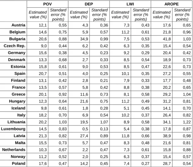
3.1. Cross-sectional measures
The estimated standard error for the AROPE lies between 0.5 and 1 percentage point in most of the countries, which means that the absolute margin of error for the indicator (based on normality assumption) is between ±1 and ±2 percentage points. The standard error is greater than 1 point in Bulgaria, Greece, Lithuania, Portugal and Romania; while it is lower than 0.5 point in Germany, Finland and Sweden. For the two latter “Nordic” countries, it seems that the impact of weight calibration on variance has been taken into account somehow.
Table 1: Estimated standard errors for the at-risk-of-poverty or social exclusion indicator (AROPE) and its three components, 2010
POV DEP LWI AROPE
Estimated value (%) Standard error (% points) Estimated value (%) Standard error (% points) Estimated value (%) Standard error (% points) Estimated value (%) Standard error (% points) Austria 12,1 0,55 4,3 0,36 7,3 0,43 17,6 0,65 Belgium 14,6 0,75 5,9 0,57 11,2 0,61 21,8 0,96 Bulgaria 20,6 0,88 34,9 0,99 7,5 0,53 41,8 1,03 Czech Rep. 9,0 0,44 6,2 0,42 6,3 0,35 15,4 0,54 Germany 15,6 0,38 4,5 0,23 9,2 0,29 20,4 0,42 Denmark 13,3 0,68 2,7 0,33 8,5 0,54 18,9 0,73 Estonia 15,8 0,61 9,0 0,53 8,5 0,47 22,6 0,73 Spain 20,7 0,51 4,0 0,25 10,1 0,35 27,2 0,55 Finland 13,1 0,42 2,8 0,21 7,9 0,33 17,7 0,48 France 13,5 0,57 5,8 0,42 8,8 0,38 20,2 0,65 Greece 20,1 0,92 11,6 0,73 8,1 0,58 29,2 1,04 Hungary 12,3 0,64 21,6 0,75 11,2 0,49 31,2 0,81 Iceland 9,8 0,61 1,8 0,28 5,1 0,45 14,1 0,70 Italy 18,2 0,70 6,9 0,54 10,2 0,37 26,4 0,82 Lithuania 20,2 1,03 19,5 1,07 8,9 0,58 34,1 1,22 Luxembourg 14,5 0,83 0,5 0,13 5,4 0,38 17,8 0,87 Latvia 21,3 0,82 27,4 0,89 11,8 0,66 38,9 0,98 Malta 15,5 0,73 5,7 0,47 8,3 0,48 21,6 0,81 Netherlands 10,3 0,67 2,2 0,47 7,3 0,61 15,8 0,88 Norway 11,2 0,52 2,0 0,25 6,3 0,37 15,4 0,57 Poland 17,6 0,47 14,2 0,45 7,4 0,27 28,7 0,54
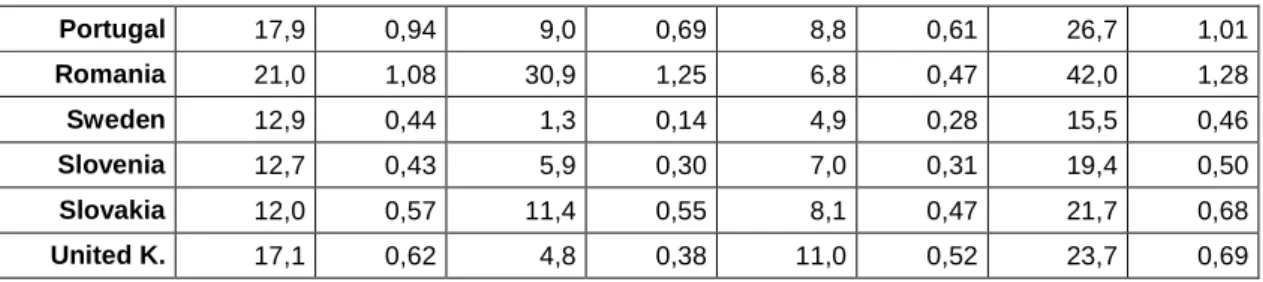
Portugal 17,9 0,94 9,0 0,69 8,8 0,61 26,7 1,01 Romania 21,0 1,08 30,9 1,25 6,8 0,47 42,0 1,28 Sweden 12,9 0,44 1,3 0,14 4,9 0,28 15,5 0,46 Slovenia 12,7 0,43 5,9 0,30 7,0 0,31 19,4 0,50 Slovakia 12,0 0,57 11,4 0,55 8,1 0,47 21,7 0,68 United K. 17,1 0,62 4,8 0,38 11,0 0,52 23,7 0,69
Source: Authors’ calculations based on the EU-SILC micro-data files provided by Net-SILC2 (Version 01-03-12)
3.2. Longitudinal measures
The relative margin of error of the persistent at-risk-of-poverty rate ranges from 14% in France to more than 50% in the Netherlands and Iceland. Compared to what we got for the AROPE (see previous), the precision of the persistent at-risk-of-poverty rate appears to be lower. There are several possible reasons for this:
• For the longitudinal component of EU-SILC, the achieved sample size is lower than for the cross-sectional component: the longitudinal sample sizes range from about 1000 individuals in Iceland to 11000 in France. This is caused mainly by the rotating design used in most of the countries, but also by losses to follow-up and attrition. Based on a rotating design, a given percentage (usually 25%) of the sample is rotated out each year and is replaced with a new subsample.
• The persistent at-risk-of-poverty rate generally takes lower value than the cross-sectional at-risk-of poverty rate (POV) or the AROPE indicator.
• The higher dispersion of the longitudinal sampling weights, which are adjusted at each wave for attrition and calibrated to external data sources.
Table 2 – Estimated values, standard errors and confidence intervals for the persistent at-risk-of-poverty rate, 2006-2009
Estimated value (%) Estimated Standard error (% points) Confidence interval - lower bound Confidence interval - upper bound Relative margin of error (%) Austria 6,1 0,78 4,6 7,6 25,1 Belgium 9,2 1,08 7,1 11,3 23,0 Bulgaria 10,7 1,44 7,9 13,5 26,4 Cyprus 11,3 1,06 9,2 13,4 18,4 Czech Rep. 3,7 0,63 2,5 4,9 33,4 Denmark 2,3 0,53 1,3 3,3 45,2 Estonia 12,9 1,04 10,9 14,9 15,8 Spain 11,4 0,87 9,7 13,1 15,0 Finland 6,5 0,76 5,0 8,0 22,9 France 6,5 0,45 5,6 7,4 13,6
Greece 16,1 1,50 13,2 19,0 18,3 Hungary 8,6 1,52 5,6 11,6 34,6 Ireland 7,7 1,49 4,8 10,6 37,9 Iceland 4,2 1,12 2,0 6,4 52,3 Italy 13,0 1,07 10,9 15,1 16,1 Lithuania 11,7 1,42 8,9 14,5 23,8 Luxembourg 8,8 1,08 6,7 10,9 24,1 Latvia 17,1 2,16 12,9 21,3 24,8 Malta 10,1 1,27 7,6 12,6 24,6 Netherlands 4,7 1,26 2,2 7,2 52,5 Norway 5,7 0,69 4,3 7,1 23,7 Poland 10,2 0,80 8,6 11,8 15,4 Portugal 9,8 1,16 7,5 12,1 23,2 Sweden 3,7 0,60 2,5 4,9 31,8 Slovenia 7,0 0,73 5,6 8,4 20,4 Slovakia 5,4 0,89 3,7 7,1 32,3 United K. 8,0 0,94 6,2 9,8 23,0
Source: Authors’ calculations based on the EU-SILC micro-data files provided by Net-SILC2 (Version 01-03-12)
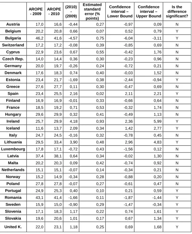
3.3. Measures of net change
In order to monitor the process towards agreed policy goals, particularly in the context of the Europe 2020 strategy, we are interested in the evolution of social indicators. However, interpreting differences between point estimates at different wave may be misleading. It is therefore necessary to estimate the standard error for these differences in order to judge whether or not the observed differences are statistically significant. A major problem arising at this stage is to take into account temporal correlations between indicators.
Estimated standard errors and confidence intervals (based on normality assumption) for net changes in the AROPE between 2009 and 2010 are shown in the next table. The computations were made within Eurostat premises using the EU-SILC Production DataBase (EU-SILC PDB). If a confidence interval does not include 0, we can say the difference in the AROPE between 2009 and 2010 is statistically significant (at a given level of confidence).
Table 3 – Estimated standard errors for estimators of net change in the AROPE between 2009 and 2010 AROPE - 2009 AROPE - 2010 (2010) - (2009) Estimated standard error (% points) Confidence interval – Lower Bound Confidence interval – Upper Bound Is the difference significant? Austria 17,0 16,6 -0,44 0,27 -0,97 0,09 N Belgium 20,2 20,8 0,66 0,07 0,52 0,79 Y Bulgaria 46,2 41,6 -4,57 0,75 -6,04 -3,11 Y Switzerland 17,2 17,2 -0,08 0,39 -0,85 0,69 N Cyprus 22,9 23,6 0,67 0,55 -0,42 1,76 N Czech Rep. 14,0 14,4 0,36 0,30 -0,23 0,96 N Germany 20,0 19,7 -0,26 0,24 -0,72 0,21 N Denmark 17,6 18,3 0,74 0,40 -0,03 1,52 N Estonia 23,4 21,7 -1,69 0,38 -2,44 -0,94 Y Greece 27,6 27,7 0,11 0,30 -0,47 0,69 N Spain 23,4 25,5 2,16 0,02 2,11 2,21 Y Finland 16,9 16,9 -0,01 0,33 -0,66 0,64 N France 18,5 19,2 0,71 0,53 -0,32 1,74 N Hungary 29,6 29,9 0,32 0,41 -0,49 1,13 N Ireland 25,7 29,9 4,18 0,93 2,36 5,99 Y Iceland 11,6 13,7 2,09 0,34 1,42 2,77 Y Italy 24,7 24,5 -0,16 0,32 -0,78 0,45 N Lithuania 29,5 33,4 3,90 0,48 2,96 4,83 Y Luxembourg 17,8 17,1 -0,72 0,43 -1,56 0,12 N Latvia 37,4 38,1 0,64 0,34 -0,02 1,30 N Malta 20,2 20,3 0,09 0,42 -0,74 0,92 N Netherlands 15,1 15,1 -0,07 0,14 -0,34 0,21 N Norway 15,2 14,9 -0,34 0,28 -0,88 0,20 N Poland 27,8 27,8 -0,07 0,27 -0,61 0,47 N Portugal 24,9 25,3 0,40 0,10 0,21 0,59 Y Romania 43,1 41,4 -1,66 0,11 -1,87 -1,44 Y Sweden 15,9 15,0 -0,90 0,29 -1,47 -0,34 Y Slovenia 17,1 18,3 1,17 0,22 0,74 1,61 Y Slovakia 19,6 20,6 1,01 0,17 0,67 1,34 Y United K. 22,0 23,1 1,18 0,25 0,69 1,68 Y
Source: EU-SILC (Production Data Base – PDB) preliminary results Note: for Austria, Luxembourg and Slovakia, the effect of stratification on variance is ignored
4. Conclusion
The approach to variance estimation which is presented in this paper is both theoretically sound and easy to implement with the existing software packages in the context of an EU-wide undertaking such as EU-SILC. The approach is able to deal with the three main kinds of indicators used in EU-SILC that is, cross-sectional and longitudinal indicators, and indicators of net changes. The linearization technique may be used to deal with complex non-linear indicators. However, the procedure is justified on the basis of asymptotic properties so estimates may not be reliable if the sample size is not sufficiently large. In addition, first-stage sampling fractions must be close to zero for the ‘ultimate cluster’ approximation to be valid (in case of multi-stage sampling designs). The numerical results shown in the previous section seem to make sense, although they must be read with caution given the lack of sampling design information in the EU-SILC user datasets and potential quality problems with the existing design variables. Eurostat is currently working with Net-SILC2 to improve this situation. Concrete recommendations have already been made by Net-SILC2 for better recording of sampling design variables.
References
Berger, Y. G. (2003). A Simple Variance Estimator for Unequal Probability Sampling Without Replacement. University of Southampton, Statistical Sciences Research Institute, Methodology Working paper M03/09.
Berger, Y. G. and Priam, R. (2013). A simple variance estimator of change for rotating repeated surveys: an application to the EU-SILC household surveys. University of Southampton, Statistical Sciences Research Institute.
Deville, J-C. (1999). Variance estimation for complex statistics and estimators: linearization and residual techniques. Survey Methodology, December 1999, 25, 2, 193-203.
Deville, J-C. and Särndal, C-E. (1992). Calibration estimators in survey sampling. Journal of the American Statistical Association, 87, 418, 376-382.
Goedemé, T. (2010). The construction and use of sample design variables in EU-SILC. A user’s perspective. Report prepared for Eurostat. Available at:
http://www.centrumvoorsociaalbeleid.be/index.php?q=node/2157/en
Osier, G. (2009). Variance estimation for complex indicators of poverty and inequality using linearization techniques. Survey Research Methods, 3, 3, 167-195.
Verma, V. and Betti, G. (2011). Taylor linearization sampling errors and design effects for poverty measures and other complex statistics. Journal of Applied Statistics, 38, 8, 1549-1576.