Atmospheric correction and surface spectral unit mapping using
Thermal Emission Imaging System data
Joshua L. Bandfield and Deanne Rogers
Department of Geological Sciences, Arizona State University, Tempe, Arizona, USA Michael D. Smith
NASA Goddard Space Flight Center, Greenbelt, Maryland, USA Philip R. Christensen
Department of Geological Sciences, Arizona State University, Tempe, Arizona, USA
Received 4 May 2004; revised 14 July 2004; accepted 18 August 2004; published 21 October 2004.
[1] Three techniques are described for the extraction of surface emissivity and
compositional information from Thermal Emission Imaging System (THEMIS) images. Synthetic images were constructed with different atmospheric properties and random and systematic errors to estimate the uncertainty in the retrieved surface emissivity. The three techniques are as follows: (1) A constant radiance removal algorithm determines and removes a constant radiance from atmospheric emission as well as systematic calibration radiance offsets. (2) Surface emissivity retrieval uses low-resolution Thermal Emission Spectrometer surface emissivity data to determine atmospheric properties for an image that can be then applied to individual THEMIS pixels. (3) A spectral unit mapping algorithm determines spectral end-member concentrations using a deconvolution routine similar to several previous applications. The initial application of these techniques to three images covering the same region of the Martian surface but at different surface temperature and atmospheric conditions yields consistent surface spectral shapes as well as end-member concentrations. Retrieved aerosol opacity information is consistent with an independently developed opacity retrieval method. The application of the techniques described here is done in a stepwise fashion and may be applied to the desired level of analysis necessary for interpretation of surface properties. INDEXTERMS:5757 Planetology: Fluid Planets: Remote sensing; 5709 Planetology: Fluid Planets: Composition; 5764 Planetology: Fluid Planets: Surfaces; 5794 Planetology: Fluid Planets: Instruments and techniques; 6225 Planetology: Solar System Objects: Mars;
KEYWORDS:atmospheric correction, infrared spectroscopy, Mars
Citation: Bandfield, J. L., D. Rogers, M. D. Smith, and P. R. Christensen (2004), Atmospheric correction and surface spectral unit mapping using Thermal Emission Imaging System data,J. Geophys. Res.,109, E10008, doi:10.1029/2004JE002289.
1. Introduction
[2] Thermal infrared observations of Mars can be used to determine the surface mineralogy. This information is essential for an accurate reconstruction of geologic and climate history of the planet. Though most rock-forming minerals have distinctive absorptions in the thermal infrared (TIR) portion of the spectrum (roughly defined here as5 – 50 mm), the Martian atmosphere also contains absorptions throughout the TIR. As a result, accurately accounting for the obscuring effects of the atmosphere is essential for any surface spectral analysis and determination of surface mineralogy.
[3] The Martian atmosphere contains absorptions due to atmospheric dust and water ice aerosols as well as water vapor and CO2 gases. The spectral response of these
absorptions are typically at least of the same order of magnitude as the signal from surface mineralogic absorp-tions. Furthermore, the atmospheric dust, being primarily composed of silicate materials, has broad absorptions in the 10 and 20mm regions of the spectrum similar in character to silicate surface materials.
[4] A number of methods have been developed for use with Thermal Emission Spectrometer (TES) data to remove the obscuring effects of the atmosphere to obtain surface emissivities. Two basic surface-atmosphere separation algo-rithms have been developed [Smith et al., 2000a] on the basis of the consistency of atmospheric spectral shapes [Bandfield et al., 2000a]. A third algorithm was developed that uses multiple emission angle TES observations to directly calcu-late surface emissivity and atmospheric opacity [Bandfield and Smith, 2003]. This method requires fewer assumptions about the behavior of the atmosphere and surface but also requires special observations and can only be applied to a fraction of the TES data set. Finally, a ratio of two different
Copyright 2004 by the American Geophysical Union. 0148-0227/04/2004JE002289$09.00
surfaces with similar atmospheric characteristics is a simple method for canceling most of the atmospheric effects present, resulting in a spectrum that is dominated by the ratio of the two surface emissivities [Ruff and Christensen, 2002]. These four independently developed methods are in good agree-ment with each other, and Martian surface emissivities in the TIR are well characterized.
[5] Spectral unit mapping with TES data has used simple band indices to produce qualitative maps [Bandfield, 2000;
Christensen et al., 2000;Ruff and Christensen, 2002]. The output of the deconvolution atmospheric correction algo-rithm [Smith et al., 2000a] has been used to produce quantitative mineral and spectral unit abundance maps [Bandfield et al., 2000b; Bandfield, 2002; Rogers and Christensen, 2003; Hamilton et al., 2003]. In addition to high spectral resolution/low spatial resolution TES data the 2001 Mars Odyssey Thermal Emission Imaging System (THEMIS) instrument provides complimentary low spec-tral/high spatial resolution data for the analysis of Martian surface properties. The high spatial resolution imaging capability of THEMIS is similar in nature to terrestrial multispectral TIR instruments such as the thermal infrared multispectral scanner (TIMS), Advanced Spaceborne Ther-mal Emission and Reflection Radiometer (ASTER), and the Moderate Resolution Imaging Spectroradiometer (MODIS) and ASTER simulator (MASTER). Spectral index and deconvolution techniques have been applied to these data sets for the quantitative mapping of a variety of surface compositions on Earth [e.g., Gillespie, 1992; Hook et al., 1994; Crowley and Hook, 1996; Ramsey et al., 1999;
Ramsey and Fink, 1999;Ramsey, 2002].
[6] This work describes atmospheric correction and spec-tral unit mapping techniques as they are specifically applied to THEMIS data. It is possible to take advantage of the spatial information present within a THEMIS image as well as previous low spatial resolution surface emissivities retrieved from TES data in order to retrieve high spatial resolution surface emissivity from a THEMIS image. After retrieval of surface emissivity it is possible to obtain quantitative mineralogic and petrologic unit maps using a linear least squares fit of spectral end-members to each THEMIS pixel. The methods and techniques described here allow for the analysis of high-resolution compositional information using THEMIS data.
2. Approach
[7] Section 2 covers four basic themes: (1) a brief tion of the THEMIS instrument and operations, (2) a descrip-tion of the atmospheric correcdescrip-tion and spectral unit mapping methods as they are applied to the THEMIS data, (3) a description of a number of sources of uncertainty and their impact on the THEMIS data, and (4) an analysis of synthetic data with estimates of a number of error sources to determine the expected precision and accuracy of the THEMIS data.
2.1. THEMIS Instrument Description
[8] The THEMIS instrument consists of TIR and visible/ near-infrared multispectral imagers. The TIR imaging por-tion of THEMIS consists of an uncooled 320 by 240 element microbolometer array with nine spectral channels centered from 6.5 to 15mm. Images are assembled in a push
broom fashion with subsequent lines in the array coadded within each spectral channel to increase the signal-to-noise ratio. Spatial sampling is 100 m from the Mars Odyssey 420 km altitude circular orbit. Local times of observation range from 0300 to 0600 and 1500 to 1800 LT. A detailed description of the THEMIS instrument is provided by
Christensen et al.[2003].
[9] An internal calibration flag and instrument response functions determined from prelaunch data are used to produce calibrated radiance images. THEMIS has a single-pixel noise equivalent spectral radiance of 2.72 106W cm2sr1mm1in band 9, corresponding to a 1-s
noise equivalent delta temperature of0.4 at 245 K and 1.1 at 180 K [Christensen et al., 2003].
2.2. Methods
2.2.1. Atmospheric Correction
2.2.1.1. Constant Radiance Offset Removal
[10] Quantitative analysis of THEMIS TIR data requires accounting for atmospheric effects, even if only relative differences between regions within an image are investi-gated. The observed Martian radiance measured by TES can be described by equation (1):
Iobsð Þ ¼v eð ÞvB T½ surf;vet0ð Þv=mþ Zt0 0 B T p½ ð Þ;vetðv;pÞ=mdt n o : ð1Þ
[11] In this equation, Iobs(v) is the measured radiation; e(v) is the surface emissivity; B[Tsurf, v] is the blackbody radiance as a function of surface temperature,Tsurf;t(v,p) is the normal opacity profile as a function of wavelength and pressure; and m is the cosine of the emission angle. The integral is taken through the atmosphere from the opacity at the spacecraft (t= 0) to the surface (t= t0); T(p) is the atmospheric temperature profile. The first term accounts for the absorption of surface radiation by the atmosphere; the second (integral) term accounts for radiation emitted by the atmosphere and suspended aerosols. Solar and thermal radiation reflected from the surface as well as secondary scattering are neglected in this equation, and surface radi-ation is considered to be diffuse. In addition, this model assumes that the dust is well mixed with the CO2gas and not stratified at any level in the atmosphere. The effects of these assumptions are discussed by Smith et al. [2000b],
Bandfield and Smith[2003], andSmith et al.[2003]. [12] The two terms in equation (1) can be thought of as a proportional term (atmospheric attenuation of surface radi-ance) and an additive term (atmospheric emission). The radiative contribution of the atmospheric emission is inde-pendent of surface temperature and must be removed to compare the spectral response of surfaces of different temperatures. This effect is apparent and often dominant in equivalent emissivity images of sunlit (warm) and shaded (cold) slopes of a surface of uniform composition because the relative contribution of the atmospheric emission will be greater over cold surfaces.
[13] The first step in THEMIS image atmospheric cor-rection is the calculation and removal of the atmospheric emission term. This contribution can be calculated directly
from the THEMIS TIR calibrated radiance data using a region (that typically contains several thousand pixels) of assumed constant emissivity and variable temperature. For each pixel within the surface of uniform emissivity the measured radiance can be modeled by the following:
Iobsðv;nÞ ¼A vð ÞB T½ surf;v;n þC vð Þ; ð2Þ
where Iobs(v,n) is the measured radiance for each spectral channel (v) and pixel (n); A(v) is a multiplicative term representing surface emissivity and atmospheric attenuation of surface radiation; B[Tsurf,v, n] is the Planck radiance at the kinetic temperature of the surface, Tsurf, for each pixel; andC(v) is the constant radiance term due to atmospheric emission.
[14] B[Tsurf,v] is obtained for each pixel by assuming that the spectral channel of the highest brightness temperature is the surface kinetic temperature. With this assumption, there are only two unknowns for each spectral channel with typically thousands of measurements. A(v) and C(v) are determined using an iterative non-linear least squares algo-rithm, andC(v) is subtracted from the entire radiance image for each spectral band.
[15] The constant radiance correction is similar in nature to that described by Young et al. [2002] for application to airborne hyperspectral thermal infrared Spatially Enhanced Broadband Array Spectrograph System data. The methods of
Young et al.[2002] have been applied to TES and THEMIS data in a preliminary manner [Mustard, 2004;Kirkland et al., 2002]. As it is applied here, this method is calculated directly from a selected area of the data rather than from a scatterplot, as that fromYoung et al.[2002], and is used for removal of the atmospheric emission only. Other aspects of the atmospheric correction described byYoung et al.[2002] are not applicable here because it requires unit emissivity at each wavelength in some location within an image. Unit surface emissivity rarely occurs at many THEMIS wavelengths for most Martian surfaces [e.g.,Bandfield and Smith, 2003].
[16] After this correction, spectral differences between surfaces are no longer influenced by surface temperature differences. Relative differences between equivalent emis-sivity spectra are accurate and are not influenced by atmospheric effects. Ratios and relative differences within emissivity images represent those of the surfaces being measured.
[17] The quality of the correction can be assessed by inspecting the corrected equivalent emissivity image. Topo-graphic features should not be readily apparent in the corrected image. While surface mineralogy can be associ-ated with topographic features, it is not common for mineralogy to be associated with sunlit and shaded slopes.
2.2.1.2. Surface Emissivity Retrieval
[18] The constant radiance offset removal greatly simpli-fies the problem of atmospheric correction. With the effects of atmospheric emission removed, the atmospheric temper-ature profile described by the second term of equation (1) is no longer necessary for the correction and can be performed using a single multiplicative term for each spectral channel. [19] Previous atmospheric correction methods using TES data have relied on significant spectral differences between the surface and atmosphere at wavelengths greater than 18 mm [Smith et al., 2000a] or multiple emission angle
observations [Bandfield and Smith, 2003]. These observa-tions are not available for use with THEMIS data, and a different method must be devised for determining the contributions of the atmosphere to the measured spectra.
[20] A simple correction method uses surface emissivity spectra retrieved from TES data to determine atmospheric contributions for a large area of a THEMIS image. The determined atmospheric contributions can then be removed for the entire image.
[21] Greater than 99% of the Martian surface can be accurately described by three spectral shapes [Bandfield et al., 2000a; Bandfield, 2002; Bandfield and Smith, 2003]. These surface spectral units, especially surface dust, typi-cally cover large uniform areas that can be accurately defined at the spatial resolution of the TES instrument. This property allows for the surface emissivity of a portion of a THEMIS image to be defined using TES data in order to determine the atmospheric contribution. This contribution can then be removed on a pixel by pixel basis from the entire THEMIS image, allowing for the resolution of mineralogically unique surfaces that are not spatially re-solvable by TES.
[22] This method as well as the constant radiance correc-tion makes the assumpcorrec-tion that the atmosphere is not spatially variable over the THEMIS scene. This assumption generally applies to atmospheric dust outside of periods of major dust storm activity or large elevation differences. Variable dust opacities are expected in areas of a variety of elevations because opacity is generally proportional to surface pressure. As a result the atmospheric correction must be applied to regions of similar elevation in an image. Water ice can also be highly variable at small spatial scales and can be accounted for in the spectral unit mapping algorithm described below.
2.2.2. THEMIS Spectral Unit Mapping
[23] Concentration maps of individual spectral compo-nents have been used for interpretation of a wide variety of visible through TIR imaging data sets [Adams et al., 1986;
Mustard and Pieters, 1987;Blount et al., 1990;Smith et al., 1990; Sabol et al., 1992; Gillespie, 1992; Ramsey et al., 1999;Ramsey and Fink, 1999;Ramsey, 2002]. The method applied here is similar to that applied to other TIR data sets. A linear least squares fit of selected end-members to individual atmospherically corrected THEMIS pixels is performed, and the concentrations of each of the end-members is retrieved. The surface end-member spectral shapes can come from a variety of sources, including laboratory measurements and TES data convolved to the THEMIS spectral band passes or directly from the THEMIS surface emissivity image. The RMS error between the model fits and the measured spectra is also calculated. Both the concentrations and the errors are in image format, and the spatial distributions can be interpreted.
[24] The technique as it is applied here is similar to the deconvolution method ofRamsey and Christensen [1998] andRamsey et al.[1999] with modifications byBandfield et al. [2000b]. Each pixel of an image is independently deconvolved using a fixed set of end-members. The pro-gram is an iterative algorithm that successively removes surface component concentrations that are less than zero until the resulting concentrations are all positive or zero. A blackbody component is included in the least squares fit to
account for variable amounts of spectral contrast. Negative concentrations of blackbody are allowed to account for surface spectral components with greater spectral contrast than the selected end-members.
[25] The number of end-members used in the spectral unit mapping must be limited to less than the number of bands used for the deconvolution. In addition, the number of independent components is further reduced because a single band (typically THEMIS band 3) is chosen for temperature determination and set to a fixed emissivity value. Using THEMIS bands 3 thorough 9 as is applied here, no more than five end-members including blackbody should be used in the spectral unit mapping routine.
2.2.3. Individual Pixel Water Ice Correction
[26] It is not uncommon for water ice to be spatially variable within individual THEMIS images. When this is the case, the above two atmospheric removal strategies only remove the average amount of water ice in the entire image or training region and will overcorrect or under correct for water ice within individual THEMIS pixels. The spectral unit mapping algorithm may be used to remove the spatially variable water ice contribution to the THEMIS data.
[27] The Martian surface and atmospheric spectral com-ponents have been demonstrated to combine in a linear manner [Bandfield et al., 2000a] and a least squares fit of surface, atmospheric components may be used to retrieve the spectral response caused by the atmospheric compo-nents, and their contributions may be removed [Smith et al., 2000a; Bandfield et al., 2000b; Bandfield, 2002]. This retrieval method may be employed if a water ice spectral shape is included as an end-member in the spectral unit mapping routine. The concentration map of the water ice is multiplied by the water ice spectral shape and subtracted from the THEMIS emissivity image, and the water ice concentration map multiplied by a blackbody spectrum is added to the image. The resulting emissivity image is then corrected for spatially variable water ice.
[28] Though this method may be theoretically applied to correct for atmospheric dust as well, there is little difference in spectral shape between the dust and coarse particulate silicate surfaces on Mars within the THEMIS wavelength coverage. This makes it difficult to distinguish between the two spectral shapes and effectively determine the abundance of atmospheric dust with reasonable precision.
2.3. Uncertainties
[29] There are several sources of random and systematic noise present in THEMIS data. While most of this noise can
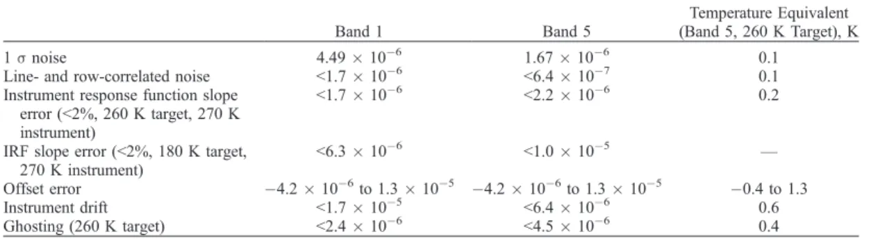
be removed for any given THEMIS scene, it is important to document and quantify its effects on surface spectral anal-ysis. Radiance uncertainties are listed in Table 1. In addi-tion, the atmospheric model and surface emissivity retrieval method also contain assumptions that result in errors that must also be quantified.
2.3.1. Signal-to-Noise Ratio
[30] The 1 s noise equivalent spectral radiance for the THEMIS instrument varies from 1.67 106 to 4.49 106 W cm2 sr1 mm1 for bands 5 and 1, respectively, corresponding to a noise equivalent delta emissivity of 0.00538 and 0.0306, respectively, at 245 K (P. R. Christensen, THEMIS calibration report, available at http:// themis-data.asu.edu/pds/calib/calib.pdf). These uncertainties are significant for single-pixel analysis but are reduced for areas covered by a number of pixels. This is typical for most areas of interest within THEMIS images, and these areas can be averaged to increase the signal-to-noise ratio.
2.3.2. Column- and Row-Correlated Noise
[31] Column-correlated noise occurs because of minor changes in detector response relative to the prelaunch response function. Row-correlated noise occurs because of minor fluctuations in detector readout bias voltage. These noise sources can cause digital number (DN) levels along a row or a column within a THEMIS image to display deviations of ±1 DN corresponding to ±3.2 106 and 8.6 106 W cm2 sr1 mm1 in bands 5 and 1, respectively. These deviations are detected and reduced in the standard THEMIS calibration to <0.2 DN (Table 1). The line- and row-correlated noise results in plaid patterns apparent in decorrelation stretch multispectral images.
2.3.3. Instrument Response Function Slope Errors
[32] The THEMIS instrument response function was defined using measurements of blackbody targets of a variety of temperatures in a vacuum chamber. The instru-ment response function displays no detectable variation over the range of operational instrument temperatures. Direct comparison with simultaneous TES observations, space observations, and CO2 polar cap images indicates that the slope of the response function is accurate to within 1 – 2%. Any radiance error present because of an incorrect slope in the instrument response function is scaled to the difference between the instrument and target temperatures and is largest for cold surfaces such as the solid CO2polar caps (Table 1).
2.3.4. Offset Errors
[33] An additional calibration uncertainty is present in setting the offset level using the instrument calibration flag.
Table 1. Systematic and Random Noise Sources Present in THEMIS Dataa
Band 1 Band 5
Temperature Equivalent (Band 5, 260 K Target), K
1snoise 4.49106 1.67106 0.1
Line- and row-correlated noise <1.7106 <6.4
107 0.1
Instrument response function slope error (<2%, 260 K target, 270 K instrument)
<1.7106 <2.2106 0.2
IRF slope error (<2%, 180 K target, 270 K instrument) <6.3106 <1.0105 — Offset error 4.2106to 1.3105 4.2106to 1.3105 0.4 to 1.3 Instrument drift <1.7105 <6.4 106 0.6 Ghosting (260 K target) <2.4106 <4.5106 0.4 a
There are several possible sources that can contribute an additive error of constant radiance to a THEMIS image, including the lack of a full aperture calibration surface observation, rapid detector temperature drift as the calibra-tion flag is being closed, incorrect retrieval of the peak shutter closing DN value, and temperature error present on the reference surface. Typical errors range from 1 to +3 DN before the application of the constant radiance offset removal algorithm.
[34] The constant radiance offset removal algorithm can remove some of this error. This correction will only be to the level present relative to the spectral band used for temperature determination (typically THEMIS band 3). As a result the offset error is a constant radiance for all bands and is usually tied to the error estimated to be present for band 3 (Table 1).
2.3.5. Wobble and Drift
[35] Time-dependent temperature changes in the detector array cause ±1 DN offsets over spatial frequencies of50 – 200 lines within an image. These offsets result in apparent horizontal spectral variations (‘‘wobble’’) when images are assembled in their proper spatial (rather than temporal) orientation. In addition, a low temporal frequency temper-ature drift is present because of the constantly changing position of the instrument relative to the Sun within its orbit as well as the changing temperature of the target. The magnitude of this drift is typically less than ±10 DN on the dayside and ±5 DN nightside. These offsets can be determined from band 10, centered within the 15 mm CO2 fundamental absorption, which does not display high spatial frequency temperature variations. After correction, total error is estimated to be <2 DN for the first line of an image to zero for the last line of the image (Table 1).
2.3.6. Ghosting
[36] ‘‘Ghosts’’ of surface features are present down track from the original in THEMIS images. These image artifacts are due to an unbaffled internal reflection present causing stray light to reach the TIR detector array and result in radiance errors of 0 – 5%. This error is dependent on the band as well as the temperature variability up track from the area of interest. The behavior of these image artifacts is modeled and is removed in the standard THEMIS calibra-tion (P. R. Christensen, THEMIS calibracalibra-tion report, avail-able at http://themis-data.asu.edu/pds/calib/calib.pdf). Some residual effect (0 – 1%, Table 1) can still be present in the corrected image, as will be discussed in section 3.3.
2.4. Error Analysis
2.4.1. Synthetic Scene Construction
[37] In order to gain an understanding of the combined effect of the various error sources on retrieved surface temperatures and spectra a synthetic image was constructed including estimates of the various uncertainties (described in detail in this section). A typical 2 min (3600 line) THEMIS scene was used to provide realistic spatial vari-ability. Average surface kinetic temperature was set to 260 K with variability from 234 to 273 K. Planck radiances were calculated for each THEMIS channel. Surface emissivities were set by multiplying the top and bottom halves of the radiance images by low- and high-albedo surface spectral emissivities [Bandfield and Smith, 2003] convolved to the THEMIS spectral band passes.
[38] Using the THEMIS convolved dust opacity spectral response [Bandfield and Smith, 2003], a synthetic radiance as measured from the top of the atmosphere was constructed using equation (1). Two conditions were simulated: (1) a warm atmosphere with a peak 9mm opacity of 0.25 and (2) a cool atmosphere more typical of THEMIS observations to date [Smith et al., 2003] with an opacity of 0.15. The effects of multiple scattering are ignored in this reconstruction, resulting in an opacity error of10% [Bandfield and Smith, 2003]. The effect of multiple scattering can be approximated by an additional additive term for a given THEMIS scene and would be accounted for by the constant radiance removal algorithm. The multiple scattering term is very nearly constant for the narrow field of view of the THEMIS instrument (M. Wolff, personal communication, 2004) and is removed as effectively as aerosol emission.
[39] The effects of random noise, row- and line-correlated noise, and detector temperature drift were obtained from a THEMIS polar image of solid CO2of constant temperature. The average radiance of the last line of the image was subtracted from each spectral channel, and any variability in the image is assumed to be due to one of these three effects. Random noise is similar to values discussed in section 2.3.1 and listed in Table 1. Residual line- and row-correlated noise is approximately ±0.2 DN. Residual drift and wobble present varies from 0 at the last line of the image to +1 DN at the first line of the image. The resulting radiance image was added to the synthetic image.
[40] A 2% instrument response error across all spectral channels was added to the synthetic data assuming an instrument temperature of 270 K. Finally, a 1.5 or 3 DN offset error was added to each spectral channel.
[41] Two synthetic images (one, high atmospheric opacity and offset error and two, normal opacity and offset error) were processed using the constant radiance removal algo-rithm and converted to equivalent emissivity and a maxi-mum brightness temperature image. These images were then compared to the original surface temperatures, equiv-alent emissivities, and ratio of the emissivities of the two surface types.
2.4.2. Temperature Errors
[42] The maximum brightness temperature can be used as an estimate of surface kinetic temperature. Comparison of the estimated surface temperature from each of the two synthetic images with the original kinetic surface temper-ature was used to give an estimate of tempertemper-ature uncertainty. The image with high atmospheric opacity and offset error contained temperature errors of 3.8 to +2.4 K with an average absolute error of 0.5 K and a standard deviation of 0.4 K. The image with normal atmospheric opacity and offset error contained tempera-ture errors of 1.9 to +2.5 K with an average absolute error of 0.9 K and a standard deviation of 0.4 K. The relative effects of typical offset errors with absorption of surface radiation by atmospheric opacity tend to cancel each other out. The offset errors are commonly positive, causing an overestimation of surface temperature, and the atmosphere is not completely transparent in any THEMIS band, resulting in an underestimate of surface tempera-ture. The relative effects of typical offset errors with absorption of surface radiation by atmospheric opacity tend to be of a similar magnitude (but opposite sign) and
cancel each other out. This occurs in THEMIS bands 3 and 9, which are most commonly the bands of highest brightness temperature.
2.4.3. Spectral Errors
[43] To determine absolute spectral errors, the constant radiance correction was applied to the two synthetic images. To obtain equivalent emissivity [eequiv(v)], each pixel was divided by the Planck curve of the highest brightness tem-perature. Each pixel can now be represented by equation (3):
eequivð Þ ¼v eð Þvet0ð Þv=m: ð3Þ
[44] The term in equation (3) is essentially surface emis-sivity multiplied by atmospheric transmisemis-sivity. For compar-ison, equivalent emissivity images were directly calculated from equation (3) without random or systematic errors or the constant radiance removal algorithm.
[45] It is necessary to compare the original and synthetic images in this form because the surface emissivity retrieval algorithm ties the data to a fixed shape, removing a large portion of the error in the process. Absolute emissivity errors do not apply to any of the surface analysis techniques described here; however, they do provide an estimate of the absolute calibration level of THEMIS and may apply to other surface emissivity analysis techniques.
[46] For spectral error analysis, three locations within each surface type were chosen. The low-albedo surface type consists of 247, 260, and, 263 K surfaces. The high-albedo surface type consists of 251, 257, and 266 K surfaces. High and low temperatures represent the range for the image, and the moderate temperatures represent typical surface temper-atures for the image. Each location is an average of at least 100 pixels to isolate systematic errors.
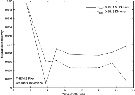
[47] This analysis indicates that absolute uncertainties are independent of surface temperature and type. However, the retrieved spectral shapes are affected by atmospheric opac-ity. Errors are similar for the and high-opacity and low-and high-error images, ranging from <0.01 to 0.05 and commonly from 0.02 to 0.03 (Figure 1).
[48] The standard deviation in equivalent emissivity for the images was calculated for the 257 and 260 K surfaces. This is 0.008 for bands 3 – 9 and 0.02 for THEMIS bands 1 and 2 (Figure 2).
[49] Relative emissivity errors were calculated from the same processed data as the absolute errors discussed above in this section. In this case, the low-albedo surface type was ratioed against the high-albedo surface type. A variety of surface temperature combinations were used for the ratios. [50] The largest errors occur in the ratios of surfaces with the greatest temperature differences. The ratio of the 247 versus the 266 K surfaces produces emissivity errors of 0 – 0.02 for bands 3 – 9 with significant changes in the spectral character (Figure 3). Relatively large errors of0 – 0.01 also occur in the ratios of cold surfaces. However, the spectral shape is not modified significantly in this case. Errors of0.01 – 0.03 are present in bands 1 and 2.
[51] Errors are smaller for ratios involving the warmer surfaces. The relative emissivity errors are 0 – 0.003 for the low-opacity and low-error images and0 – 0.005 for the high-opacity and high-error images and 0.01 in bands 1 and 2 (Figure 3).
2.4.4. Surface Emissivity Retrieval Error
[52] The error in the surface emissivity retrieval is similar to the relative emissivity errors discussed in section 2.2.3. This is because a portion of the image is fixed to a known spectral shape, removing systematic errors that are present in the THEMIS data. Misregistration between TES and THEMIS data combined with variability in surface emis-sivity can be a source of error. However, many surfaces (especially dusty regions) of Mars display nearly constant emissivities (<0.002) over areas larger than several hundred kilometers and can be typically found in THEMIS data. In addition, there are errors intrinsic to the known spectral shape retrieved from the TES data. These uncertainties have been described bySmith et al.[2000a],Bandfield and Smith
[2003], and Ruff and Christensen [2002] through the comparison of independently developed atmospheric cor-rection and surface analysis techniques. These errors are <0.005 in emissivity throughout the THEMIS spectral coverage.
2.4.5. Spectral Unit Mapping Error
[53] Errors in the surface unit concentrations are highly dependent on the end-members chosen for the deconvolu-tion. For example, concentrations from an end-member selected from the image itself will have relatively small errors. End-members selected from laboratory data, which may have substantial spectral differences from the actual end-members present in a THEMIS scene, can have larger potential errors.
[54] It is difficult to assess the uncertainty in unit con-centration from the THEMIS data themselves without additional information. However, the application discussed here is similar to terrestrial multispectral TIR studies with similar uncertainties in surface emissivity retrieval [Ramsey et al., 1999; Ramsey and Fink, 1999; Ramsey, 2002].
Ramsey [2002] degraded TIMS data over Meteor Crater, Arizona, to THEMIS spatial resolution and identified con-centration errors of 15% areal coverage. This error estimate is highly dependent on the degree of subpixel mixing and the spectral contrast between the end-members present. Some indication of the uncertainties in the methods dis-cussed here can also be estimated from the application to surfaces covered in multiple images under variable surface temperature and atmospheric opacity conditions, which is described in sections 3.2, 3.3, and 3.4.
3. Results
3.1. Image Description
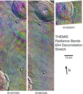
[55] Three images were selected that cover a single location on the surface as an example application of the methods described here (Figure 4). The location chosen is the northern unnamed crater (centered at 19.90N, 65.85E) of a pair in north Syrtis Major that display spectral signa-tures indicative of a lithology dominated by quartz and feldspar in and near the central peaks surrounded by a low-albedo basaltic unit [Bandfield et al., 2004]. The crater is 30 km in diameter, and the floor is 1000 m lower than the surrounding terrain, which does not have a high degree of topographic variability. The spectral signatures and their distributions present in the region are well suited for the atmospheric correction and spectral unit analysis tech-niques. The actual analysis of surface mineralogy and
discussion of formation mechanisms is discussed by
Bandfield et al.[2004].
[56] The image identification numbers used in this exam-ple are I01221005, I01920047, and I07887026. All three images were acquired under relatively low atmospheric dust and water ice opacity conditions. Dust opacities at 9mm are 0.15 – 0.20 for I01221005 and I07887026 and 0.09 for I01920047 [Smith et al., 2003]. Water ice opacities are negligible for I01221005 and I07887026 and <0.05 for I01920047. Surface temperatures for the spectral units discussed here are 260 – 265 K for I01221005 and I01920047. Surface temperatures are colder (230 K) for I07887026 because the local solar time of the Mars Odyssey orbit drifted later after the start of the mission.
3.2. Constant Radiance Correction
[57] Regions with no apparent spectral variability but with variable surface temperatures were selected for the
determination of the constant radiance correction. A 60 pixel square region containing a small crater immediately to the southwest of the main crater was selected for both I01221005 and I07887026. A 50 pixel square region con-taining the southwest rim of the main crater was selected for I01920047 because the small crater is adjacent to the corner of the image.
[58] The radiance correction values are similar for the three images. The spectral shapes are similar to the atmospheric dust, and the magnitudes of the values are consistent with the retrieved 9mm opacities (Figure 5). A significant deviation from the dust spectral shape occurs in THEMIS bands 1 and 2. The large correction values are inconsistent with the relatively low atmospheric opacities at these wavelengths.
[59] Each of the equivalent emissivity images displayed clear temperature effects without the constant radiance correction. The temperature effects are significantly reduced in the same images with the application of the constant
Figure 1. Comparison of original synthetic spectral shapes (solid) with those retrieved after application of estimated uncertainties and the constant radiance correction technique (dashed). The (top) typical opacity and DN offset error example and (bottom) high-opacity and DN offset error example are shown.
Figure 2. Standard deviations in emissivity for the synthetic image data for the typical (solid) and high (dashed) opacity and error examples. The band 3 standard deviation is close to zero in the low-error example because it was the band used for temperature determination, and the emissivity was set to unity in most of the pixels in the image.
Figure 3. Comparison of original synthetic spectral ratios (solid) with those retrieved after application of estimated uncertainties and the constant radiance correction technique (dashed). Ratios of surfaces with disparate temperatures are shown on the left, and ratios of surfaces with similar temperatures are shown on the right.
radiance correction (Figure 6). The variation in emissivity along a transect of a small crater identified in Figure 6 is reduced from 0.05 to 0.02 and 0.16 to 0.03 for bands 5 and 1, respectively. The standard deviation in emissivity along the transect is reduced from 0.01 to 0.005 and 0.03 to 0.01 for bands 5 and 1, respectively. There are no systematic trends in emissivity present in the corrected data, and the standard deviation in emissivity is similar to the random
noise of the instrument (0.004 and 0.02 for bands 5 and 1 at 260 K).
3.3. Atmospheric Correction
[60] The uniform spectral signature of the plains sur-rounding the crater provides an adequate surface to use as a training region to recover the surface emissivity from the THEMIS images. The standard deviation in emissivity
Figure 4. Band 654 (projected as red-green-blue (RGB)) decorrelation stretch radiance images used in
this study. All the images have been projected to sinusoidal equal area and then rotated to make the THEMIS image vertical on the page. Images I01221005 and I07887026 have been cut to the area of interest. Image I01920047 is an 8 s atmosphere campaign image and is displayed in its entirety.
Figure 5. Retrieved constant radiance correction values for I01221005 (solid), I01920047 (dashed), and I07887026 (dash-dotted).
within this region in the THEMIS images is 0.005 and 0.01 for bands 5 and 1, respectively. This is similar to the standard deviation due to random noise of the instrument (0.004 and 0.02 for bands 5 and 1 at 258 K) and displayed in the synthetic image example (Figure 2) indicating that there is little spectral variability.
[61] TES spectra were acquired (orbit counter keeper 2596, incremental counter keeper 1936 – 1939) over the plains surfaces south of the crater, and the surface emissivity was recovered using the deconvolution method as described by Smith et al. [2000a], Bandfield et al.
[2000b], and Bandfield [2002]. The resulting surface spectral shape (which is displayed by Bandfield et al.
[2004]) was convolved to THEMIS spectral resolution. This spectral shape was fixed as the surface emissivity for the spectrally uniform plains to the south of the crater in each of the constant radiance corrected THEMIS images, allowing for the recovery of the atmospheric opacity spectra (Figure 7).
[62] The atmospheric opacity spectra were then used to recover the surface emissivity for each individual THEMIS pixel in each of the images. Three surface emissivity spectral units were identified by examining color images using different band combinations as well as plotting emissivity data from a variety of surfaces and are shown in Figure 8. The plains spectral unit spectra outside of the crater display no significant variability because this unit was used as the training region in each image. The low-albedo unit within the crater is similar in shape to the plains unit, but with a greater spectral contrast. All three images display similar spectral shapes, and spectra of the same surface in images I01221005 and I01920047 display <0.01 difference in emissivity for bands 3 – 9. Image I07887026 is similar in spectral shape to the other images but has 30% lower spectral contrast. The spectrally distinct unit within the central peak of the crater displays a similar degree of spectral variability between the images as the low-albedo intracrater unit. Bands 1 – 2 display a 0.05 emissivity difference between the images for both spectral units.
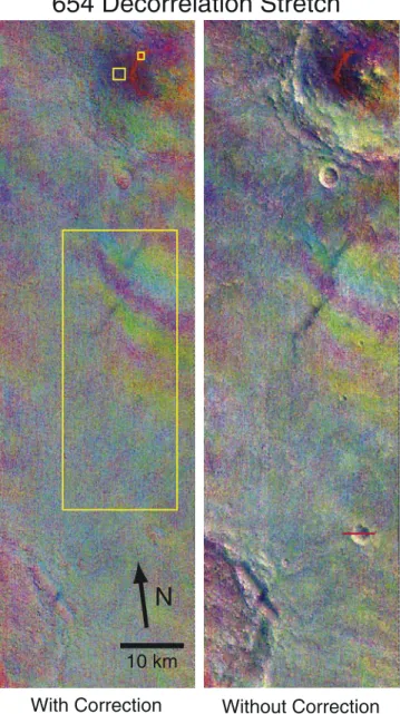
[63] The images display residual ‘‘ghost’’ features that have not been completely removed in the calibration. This is especially apparent in I01221005 to the south of the crater near the top of the image (Figures 4 and 6). This effect is due to the spatially variable warm and cold surfaces of the crater rim up track from the residual features. Individual bands are affected in different areas of the image because the stray light is detected at different angles in the THEMIS bands. This causes the color variety in the THEMIS decorrelation stretch images. The variability between the different color areas affected by the ghosting is 0.01 in emissivity, and the average of these areas is similar to other unaffected regions (Figure 9). These effects can be easily identified and avoided in the THEMIS images.
3.4. Spectral Unit Mapping
[64] Two surface spectral end-members were identified in each of the THEMIS images; the first is the plains unit spectral shape used as the known surface emissivity for the training region used in the atmospheric correction. This shape is similar to the shape of the low-albedo intracrater unit as well, and both are indicative of a basaltic surface. The second is the spectrally unique unit within the crater central peak. On the basis of interpretation of both TES and THEMIS data [Bandfield et al., 2004] a laboratory spectrum of a granitoid (quartz monzonite) convolved to THEMIS spectral resolution was selected as the end-member to map the distribution of this spectral unit.
Figure 6. Band 654 (projected as RGB) decorrelation
stretch emissivity image for I01221005. The left image was produced from data with the constant radiance correction applied. The right image is similar but without application of the constant radiance correction. The yellow boxes denote the three spectral units; the large box covers the plains spectral unit and the training area used for the surface emissivity retrieval. The small box within the purple region in the image is the low-albedo intracrater unit. The smallest box within the red region in the image is the spectrally unique central peak unit. The red line in the southeast portion of the right image indicates a transect discussed in the text.
[65] In addition to the two surface spectral units the deconvolution algorithm included an atmospheric water ice spectral shape [Bandfield et al., 2000a] and a blackbody spectral shape to account for spectral contrast differences between the end-members and the surface emissivity.
[66] The concentration maps display similar results be-tween each of the three images (Figure 10 and Table 2). The plains display moderate concentrations of the plains unit spectral shape. Higher concentrations of this shape are present in the low-albedo intracrater unit where the spectral contrast is greater. The spectrally unique unit displays high concentrations (15 – 35%) of the quartz monzonite end-member within the central peak of the crater and low concentrations (commonly <5%) outside of this region. Water ice concentrations are low in all images with average
extinctions of <0.01 and standard deviations of <0.01 for I01221005 and I01920047 and <0.02 for I07887026. This indicates that any water ice present was removed in the atmospheric correction and the water ice concentrations are not highly variable throughout each image.
[67] Average RMS errors between measured and modeled emissivity spectra are <0.005 in >98% of the pixels in I01221005 and I01920047. Higher errors often occur at areas of sharp temperature boundaries. This may indicate that effects such as a slight subpixel misregistration of the spectral bands or a high degree of anisothermality within a pixel may be present. Higher errors are present in I07887026 with an average RMS error of 0.00516. The quality of fit for regional averages remains good (Figure 11), and the higher RMS errors are due to the higher levels of
Figure 7. Retrieved atmospheric opacity spectral shapes for I01221005 (solid), I01920047 (dashed),
and I07887026 (dash-dotted). (top) Absolute opacities and (bottom) peak opacities normalized for spectral shape comparison are displayed.
random noise because of the lower temperatures present in I07887026.
4. Discussion
4.1. Constant Radiance Offset Removal
[68] Surfaces of different composition are often also at a different temperature because of a different albedo, thermal inertia, or slope relative to the Sun. The different ature contrast between the surface and atmospheric temper-atures will cause the relative differences in THEMIS emissivity data to be convoluted with temperature effects. These effects are readily apparent in THEMIS images that have been converted to equivalent emissivity without any atmospheric correction. Without correction for this effect, even qualitative spectral interpretation of THEMIS images can be problematic.
[69] The constant radiance offset removal algorithm pro-duces results that are consistent with the spectral response and level of emitting dust in the atmosphere (Figure 5) in THEMIS bands 3 – 9. Bands 1 – 2 commonly have high values determined from the algorithm. This is inconsistent with an atmospheric source because opacities are generally low in this spectral region, and a relatively cold atmosphere does not emit much radiation at 6.5mm.
[70] A likely source of this constant radiance offset is a constant error in the image calibration. This error can occur at a number of steps in the calibration process, such as the retrieval of the peak DN value from the shutter closing image (calibration reference surface) or offset error in the instrument response function. Any error of this type will result in a constant amount of radiance added to the entire image. It is not clear why this occurs frequently in THEMIS bands 1 and 2; however, the response of these two bands is
Figure 8. Surface emissivities retrieved from images I01221005 (solid), I01920047 (dashed), and
I07887026 (dash-dotted). The (top) intracrater low-albedo unit emissivity and the (bottom) spectrally unique central peak unit are shown.
lower than the other THEMIS spectral channels and would result in more prominent radiance errors for a given uncer-tainty in DN value. The offset removal algorithm will correct for these calibration errors as well as atmospheric emission sources.
[71] The constant radiance removal algorithm requires an intelligent selection of an area of variable temperature and constant emissivity. This makes it difficult to auto-mate the algorithm. It also requires the assumption of constant atmospheric properties throughout the study area in the image. This is commonly the case, but there are a number of possibly compositionally interesting areas, such as the walls of Valles Marineris, where this will be more difficult because of the highly variable atmo-spheric path lengths. An additional assumption is the determination of surface temperature from the band of highest brightness temperature. This forces a correction
relative to this band, and a portion of this constant radiance offset is mapped into surface temperature rather than the correction.
[72] Despite these limitations any surface compositional interpretation of THEMIS images needs to account for atmospheric emission. The algorithm described here requires no external information, such as an atmospheric temperature profile or opacity determination. As displayed in Figure 6, the application of the algorithm results in a clear reduction in temperature dependence, and the relative emis-sivity between spectral units is accurate.
4.2. Atmospheric Correction
[73] The spectral unit emissivities are consistent between the three images, especially I01221005 and I01920047 despite their different atmospheric opacity conditions. The spectral contrast of I07887026 is significantly shallower
Figure 9. Surface emissivity spectra within a ‘‘ghost’’ feature within the plains spectral unit. Colors in the plot refer to colored areas located within the upper right corner of the large box denoted in Figure 6.
(Figure 8) from the other two images for the intracrater spectral units, but the spectral character remains similar. The surface emissivity is qualitatively consistent for THEMIS images over a variety of temperatures (<230 – 265 K) and atmospheric conditions (tdust< 0.09 – 0.17). Fortunately or unfortunately, depending on one’s perspective, the variety of atmospheric conditions viewed by THEMIS over the course of most of a Martian year was not highly variable, and the techniques described here could not be tested under high dust opacity conditions. The conditions are typical of those used for determination of surface spectral properties using TES and THEMIS data.
[74] The cold surface temperatures and the 35 K dif-ference between I07887026 and the other images is the likely cause of the surface emissivity spectral contrast inconsistency between these images. This variability is not unexpected and is similar to the results of the uncertainty analysis discussed in section 2.4 as well as the predicted radiometric accuracy of THEMIS (P. R. Christensen, THEMIS calibration report, available at http://themis-data. asu.edu/pds/calib/calib.pdf). For quantitative analysis it is
important to compare surfaces (including the training region used for atmospheric correction) of warm (>245 K) and similar temperatures.
[75] The similarity of the results between the two warmer images as well as the uncertainty analysis indicates that the surface emissivities derived using the methods described here are accurate to <0.01 for bands 3 – 9 and retain their spectral character. It is important to maximize the surface temperatures and minimize the temperature differences between the surfaces being analyzed.
[76] Though THEMIS bands 3 – 9 are consistent and quantitatively useful, bands 1 – 2 display variability between different images and different temperatures. While it is possible to average multiple pixels to increase the SNR of these bands, small systematic errors will still cause signif-icant uncertainties in the emissivity for relatively cold surfaces. This is similar to TES data at the same wave-lengths, and the derived emissivity data are not considered trustworthy for surfaces below 275 K, and temperatures greater than 290 K are preferred for analysis [Bandfield and Smith, 2003]. It is important to use caution when
Figure 10. Spectral unit mapping concentration and RMS error images. Each end-member and RMS
error image is stretched individually with the limits of the gray scale denoted in parentheses.
Table 2. End-Member Concentrations and RMS Errors for the Three Spectral Units (Central Peak, Low-Albedo Intracrater Deposit, and Plains) in Each of the Three Images, I01221005, I01920047, and I07887026a
1221 CP 1221 LA 1221 P 1920 CP 1920 LA 1920 P 7887 CP 7887 LA 7887 P
Quartz monzonite 0.25 0.02 0.02 0.32 0.02 0.02 0.25 0.02 0.04
Plains (basalt) 0.68 1.46 0.97 0.55 1.53 0.97 0.54 1.17 0.92
Ice extinction 0.00 0.02 0.00 0.01 0.01 0.00 0.01 0.01 0.01
RMS error 0.0036 0.0023 0.0024 0.0027 0.0022 0.0025 0.0028 0.0041 0.0043 aCP is central peak, LA is low-albedo intracrater deposit, and P is plains.
interpreting data from these spectral bands; however, the data can be useful when comparing warm surfaces of similar temperature within an image.
4.3. Spectral Unit Mapping
[77] It is possible to use spectral emissivity data from a variety of sources (laboratory, TES, THEMIS) and closely fit THEMIS spectral emissivities from individual pixels. The resulting concentrations retrieved from the deconvolution are consistent between each of the three images. Only the low-albedo crater floor material displays highly variable concen-trations (Table 2) due to the significantly shallower spectrum in image I07887026. The plains unit end-member concen-trations are similar between each of the three images, as expected, and the quartz monzonite concentrations within the central peak unit vary by <0.07 between the three images.
[78] The interpretation of what the concentration repre-sents can be ambiguous. Strictly, the concentration is the weighting of the spectral shape used in the deconvolution. When all components in the end-member set have a similar surface texture, and the components present within the mixed surface are also similar in surface texture, then the concentrations closely follow their areal abundance on the surface. However, in the case presented here, a broken rock surface, a natural Martian plains surface, and water ice atmospheric particulates were used in the deconvolution. This can be a source of confusion as to the interpretation.
[79] The water ice concentrations are presented here as extinctions relative to the training region. This is the ratio of the transmitted radiation to the total source radiation at the wavelength of greatest absorption. By adding the
Figure 11. Measured (solid) versus modeled (dashed) surface emissivity spectra for the (top) intracrater low-albedo spectral unit and the (bottom) spectrally unique central peak unit. Each plot displays fits for the three example images, I01221005, I01920047, and I07887026 offset by 0.02 from top to bottom, respectively.
water ice extinction derived from the spectral unit map-ping to that derived from the atmospheric opacity spectral shape, it is possible to derive water ice opacity from the image:
tpixel¼timageln 1ð CiceÞ; ð4Þ
where tpixel is the ice opacity for the individual THEMIS pixel, timage is the water ice opacity derived from the atmospheric opacity spectral shape (this can be approxi-mated by taking the opacity from THEMIS band 8 centered at 11.75 mm), and Cice is the water ice concentration derived from the spectral unit mapping algorithm for the individual THEMIS pixel. This is a simplification in that it does not account for the variable amounts of emitted radiation from the water ice, only the emitted energy from water ice used in the training region. Though the emitted radiation is a significant effect in the atmospheric dust, it is not as large a factor with water ice because the opacities are generally lower than the dust, and the ice is at low temperatures (<185 K) that do not emit large amounts of radiation at wavelengths <12 mm. Comparisons of ice opacities derived using a similar method to that described here with those derived using a full temperature profile [Pearl et al., 2001] display results within 0.02 for water ice opacities of 0.10 – 0.15 [Bandfield et al., 2000a; Smith et al., 2000a]. Much of this difference can be attributed to the derivation techniques and spectral shapes used. The difference is <0.01 when the same analysis is used, and the only difference is the use of the temperature profile for the water ice opacity determination.
[80] As expected, plains spectral end-member concentra-tions are close to unity in the regions where they were derived from the TES data but are greater than one in the low-albedo intracrater unit. This indicates that the intra-crater unit has deeper spectral features than the plains, though the spectral shape is the same. The deeper features can be attributed to several factors: One, the plains unit has a thin cover of air fall dust that is not present in the intracrater unit because of more active saltation and cleans-ing. Thin dust covers will reduce the spectral contrast of a surface [Johnson et al., 2002;Graff et al., 2002]. Two, there are textural or particle size differences between the plains unit and the intracrater low-albedo unit. Rougher surfaces and finer particle sizes generally have lower spectral con-trast. Three, there is a contribution within the plains of a nearly blackbody component. This may be similar to indurated surfaces such as those within Pollack Crater [Ruff et al., 2001].
[81] The granitic end-member concentrations are relative to those of a broken rock surface, which has40% greater spectral contrast relative to coarse particulate surfaces [Ruff, 1998]. The thermal inertia of this spectral unit is similar to that of fine particulate surfaces rather than rocky or bedrock surfaces [Bandfield et al., 2004]. The quartz monzonite concentrations probably represent a lower limit on the areal abundance of the surface cover, and the areal abundance could be up to2 times the concentration.
[82] The complexities present in interpreting the concen-tration require assumptions to be made about the nature of the surfaces present. They do provide consistent numbers
between images and are quantitatively useful for their comparison as well as comparison to laboratory and TES data.
[83] The high quality of fit (Figures 10 and 11 and Table 2) in all of the images indicates that the spectral information present can be adequately described by the end-members used for the deconvolution. Average RMS errors between the measured and modeled emissivity spectra for the overlapping portions of the three images are 0.0025, 0.0025, and 0.0057 for I01221005, I01920047, and I07887026, respectively. The higher RMS errors are present in I07887026 because of the higher pixel to pixel random noise, but averages of pixels indicate that the spectral fit is as good as the other two example images (Figure 11). No other spectral compo-nents are required to describe the images.
5. Conclusions
[84] Three methods have been developed to extract con-sistent and reliable spectral surface emissivity information from THEMIS data. Surface emissivities can be determined to <0.01 for THEMIS bands 3 – 9 for relatively warm surfaces (>245 K). This allows for the determination of accurate compositional information from Martian surfaces at THEMIS spatial resolution. Specifically, the following are true:
[85] 1. Uncertainties using both random and systematic errors from both real data and processing techniques have been determined. These uncertainties are consistent with the analysis of the three example images here.
[86] 2. Images converted directly to equivalent emissivity without accounting for atmospheric emission have signifi-cant residual effects due to variable surface-atmosphere temperature contrasts.
[87] 3. The constant radiance removal technique accounts for both atmospheric emission and systematic calibration offsets, allowing for accurate relative emissivity determina-tion from surfaces of different temperatures. Removal of atmospheric emission from an image allows for radiomet-rically accurate atmospheric correction without the need for a temperature profile.
[88] 4. Atmospheric properties can be determined from relatively low spatial resolution TES data and a selected training region in the THEMIS image. The atmospheric properties can then be applied to recover surface emissivity from individual THEMIS pixels.
[89] 5. Intelligent selection of spectral end-members from a variety of sources can be used to recover consistent concentrations from which surface areal coverages can be inferred. The concentration images display coherent spatial patterns, and interpretation of distributions is more straight-forward than standard decorrelation stretch images.
[90] 6. The application of the techniques described here is done in a stepwise fashion and may be applied to the desired level of analysis necessary for interpretation of surface properties.
[91] Acknowledgments. We would like to thank Laurel Cherednik, Andras Dombovari, and Kelly Bender for cheerfully enduring our data requests and collecting excellent observations. Noel Gorelick, Michael Weiss-Malik, and Benjamin Steinberg provided essential software support for the THEMIS data set. Mike Wolff, Jeff Moersch, and John Pearl
provided useful advice and discussion. Scott Anderson and an anonymous reviewer provided helpful suggestions as formal reviewers.
References
Adams, J. B., M. O. Smith, and P. E. Johnson (1986), Spectral mixture modeling: A new analysis of rock and soil types at the Viking Lander 1 site,J. Geophys. Res.,91, 8098 – 8112.
Bandfield, J. L. (2000), Isolation and characterization of Martian atmo-spheric constituents and surface lithologies using thermal infrared spec-troscopy, Ph.D. dissertation, 195 pp., Ariz. State Univ., Tempe. Bandfield, J. L. (2002), Global mineral distributions on Mars,J. Geophys.
Res.,107(E6), 5042, doi:10.1029/2001JE001510.
Bandfield, J. L., and M. D. Smith (2003), Multiple emission angle surface-atmosphere separations of Thermal Emission Spectrometer data,Icarus, 161, 47 – 65.
Bandfield, J. L., P. R. Christensen, and M. D. Smith (2000a), Spectral data set factor analysis and end-member recovery: Application to Martian atmospheric particulates,J. Geophys. Res.,105, 9573 – 9588.
Bandfield, J. L., V. E. Hamilton, and P. R. Christensen (2000b), A global view of Martian surface compositions from MGS-TES,Science,287, 1626 – 1630.
Bandfield, J. L., V. E. Hamilton, P. R. Christensen, and H. Y. McSween Jr. (2004), Identification of quartzofeldspathic materials on Mars,J. Geo-phys. Res.,109, E10009, doi:10.1029/2004JE002290.
Blount, G., M. O. Smith, J. B. Adams, R. Greeley, and P. R. Christensen (1990), Regional aeolian dynamics and sand mixing in the Gran Desierto: Evidence from Landsat thematic mapper images,J. Geophys. Res.,95, 15,463 – 15,482.
Christensen, P. R., et al. (2000), Detection of crystalline hematite miner-alization on Mars by the Thermal Emission Spectrometer,J. Geophys. Res.,105, 9632 – 9642.
Christensen, P. R., et al. (2003), Morphology and composition of the sur-face of Mars: Mars Odyssey THEMIS results,Science,300, 2056 – 2061. Crowley, J. K., and S. J. Hook (1996), Mapping playa evaporite minerals and associated sediments in Death Valley, California, with multispectral thermal infrared images,J. Geophys. Res.,101, 643 – 660.
Gillespie, A. R. (1992), Spectral mixture analysis of multispectral thermal infrared images,Remote Sens. Environ.,42, 137 – 145.
Graff, T. G., R. V. Morris, and P. R. Christensen (2002), Effects of palagonitic and basaltic dust coatings on visible, near-IR, thermal emis-sion and Moessbauer spectra of rocks and minerals: Implications for mineralogical remote sensing of Mars, Eos Trans. AGU,83(47), Fall Meet. Suppl., Abstract P72A-0486.
Hamilton, V. E., P. R. Christensen, H. Y. McSween Jr., and J. L. Bandfield (2003), Searching for the source regions of Martian meteorites using MGS TES: Integrating Martian meteorites into the global distribution of volcanic materials on Mars,Meteorit. Planet. Sci.,38, 871 – 886. Hook, S. J., K. E. Karlstrom, C. F. Miller, and K. J. W. McCaffrey (1994),
Mapping the Piute Mountains, California, with thermal infrared multi-spectral scanner (TIMS) images,J. Geophys. Res.,99, 15,605 – 15,622. Johnson, J. R., P. R. Christensen, and P. G. Lucey (2002), Dust coatings on
basaltic rocks and implications for thermal infrared spectroscopy of Mars, J. Geophys. Res.,107(E6), 5035, doi:10.1029/2000JE001405. Kirkland, L. E., K. C. Kerr, J. Ward, E. R. Keim, J. H. Hackwell, and
J. M. McAfee (2002), Surface composition of Mars: Results from a new atmospheric correction technique applied to TES,Lunar Planet. Sci. [CD-ROM],XXXIII, abstract 1220.
Mustard, J. F. (2004), A simple approach to estimating surface emissivity with THEMIS data,Lunar Planet. Sci. [CD-ROM], XXXV, abstract 1552.
Mustard, J. F., and C. M. Pieters (1987), Abundance and distribution of ultramafic microbreccia in Moses Rock Dike: Quantitative application of mapping spectroscopy,J. Geophys. Res.,92, 10,376 – 10,390.
Pearl, J. C., M. D. Smith, B. J. Conrath, J. L. Bandfield, and P. R. Christensen (2001), Mars Global Surveyor Thermal Emission Spectro-meter (TES) observations of ice clouds during aerobraking and science phasing,J. Geophys. Res.,106, 12,325 – 12,338.
Ramsey, M. S. (2002), Ejecta distribution patterns at Meteor Crater, Arizona: On the applicability of lithologic end-member deconvolution for spaceborne thermal infrared data of Earth and Mars, J. Geophys. Res.,107(E8), 5059, doi:10.1029/2001JE001827.
Ramsey, M. S., and P. R. Christensen (1998), Mineral abundance determi-nation: Quantitative deconvolution of thermal emission spectra,J. Geo-phys. Res.,103, 577 – 596.
Ramsey, M. S., and J. H. Fink (1999), Estimating silicic lava vesicularity with thermal remote sensing: A new technique for volcanic mapping and monitoring,Bull. Volcanol.,61, 32 – 39.
Ramsey, M. S., P. R. Christensen, N. Lancaster, and D. A. Howard (1999), Identification of sand sources and transport pathways at Kelso Dunes, California using thermal infrared remote sensing,Geol. Soc. Am. Bull., 111, 636 – 662.
Rogers, D., and P. R. Christensen (2003), Age relationship of basaltic and andesitic surface compositions on Mars: Analysis of high-resolution TES observations of the Northern Hemisphere,J. Geophys. Res.,108(E4), 5030, doi:10.1029/2002JE001913.
Ruff, S. W. (1998), Quantitative thermal infrared emission spectroscopy applied to granitoid petrology, Ph.D. dissertation, 234 pp., Ariz. State Univ., Tempe.
Ruff, S. W., and P. R. Christensen (2002), Bright and dark regions on Mars: Particle size and mineralogical characteristics based on Thermal Emission Spectrometer data, J. Geophys. Res.,107(E12), 5127, doi:10.1029/ 2001JE001580.
Ruff, S. W., P. R. Christensen, R. N. Clark, H. H. Kieffer, M. C. Mailin, J. L. Bandfield, B. M. Jakosky, M. D. Lane, M. T. Mellon, and M. A. Prestley (2001), Mars’ ‘‘White Rock’’ feature lacks evidence of an aqueous origin: Results from Mars Global Surveyor,J. Geophys. Res.,106, 23,921 – 23,927.
Sabol, D. E., J. B. Adams, and M. O. Smith (1992), Quantitative subpixel detection of targets in multispectral images,J. Geophys. Res.,97, 2659 – 2672.
Smith, M. D., J. L. Bandfield, and P. R. Christensen (2000a), Separation of surface and atmospheric spectral features in Mars Global Surveyor Thermal Emission Spectrometer (TES) spectra,J. Geophys. Res.,105, 9589 – 9608. Smith, M. D., J. C. Pearl, B. J. Conrath, and P. R. Christensen (2000b), Mars Global Surveyor Thermal Emission Spectrometer (TES) observa-tions of dust opacity during aerobraking and science phasing,J. Geophys. Res.,105, 9539 – 9552.
Smith, M. D., J. L. Bandfield, P. R. Christensen, and M. I. Richardson (2003), Thermal Emission Imaging System (THEMIS) infrared observa-tions of atmospheric dust and water ice cloud optical depth,J. Geophys. Res.,108(E11), 5115, doi:10.1029/2003JE002115.
Smith, M. O., S. L. Ustin, J. B. Adams, and A. R. Gillespie (1990), Vegeta-tion in deserts: I. A regional measure of abundance from multispectral images,Remote Sens. Environ.,31, 1 – 26.
Young, S. J., B. R. Johnson, and J. A. Hackwell (2002), An in-scene method for atmospheric compensation of thermal hyperspectral data, J. Geophys. Res.,107(D24), 4774, doi:10.1029/2001JD001266.
J. L. Bandfield, Mars Space Flight Facility, Arizona State University, Tempe, AZ 85287-6305, USA. ([email protected])
P. R. Christensen and D. Rogers, Department of Geological Sciences, Arizona State University, Campus Box 871404, Tempe, AZ 85287-1404, USA.
M. D. Smith, NASA Goddard Space Flight Center, Mail Code 693, Greenbelt, MD 20771, USA.