Conditional dependence via Shannon capacity: axioms, estimators and applications

(1)

c

(2)

CONDITIONAL DEPENDENCE VIA SHANNON CAPACITY: AXIOMS, ESTIMATORS AND APPLICATIONS

BY WEIHAO GAO

THESIS

Submitted in partial fulfillment of the requirements

for the degree of Master of Science in Electrical and Computer Engineering in the Graduate College of the

University of Illinois at Urbana-Champaign, 2016

Urbana, Illinois Advisers:

Assistant Professor Sewoong Oh Professor Pramod Viswanath

(3)

ABSTRACT

We consider axiomatically the problem of estimating the strength of a condi-tional dependence relationship PY|X from a random variableX to a random variable Y. This has applications in determining the strength of a known causal relationship, where the strength depends only on the conditional dis-tribution of the effect given the cause (and not on the driving disdis-tribution of the cause). Shannon capacity, appropriately regularized, emerges as a natural measure under these axioms. We examine the problem of calculat-ing Shannon capacity from the observed samples and propose a novel fixed-k nearest-neighbor estimator, and demonstrate its consistency. Finally, we demonstrate an application to single-cell flow-cytometry, where the proposed estimators significantly reduce sample complexity.

(4)

(5)

ACKNOWLEDGMENTS

I would first like to thank my thesis co-advisors Prof. Sewoong Oh and Prof. Pramod Viswanath, without whom this thesis would not have been possible. Their sincere and patient guidance and support led me to the world of research, that benefited both my research projects and career endeavors. I also want to thank Prof. Sreeram Kannan, of the University of Washington, who contributed advice on this thesis.

I would like to thank Prof. Yuliy Baryshnikov, Prof. Maxim Raginsky and Prof. Yihong Wu (now at Yale University) for serving as my qualifying exam committee. I would not be able to pursue my Ph.D. without their help. I would like to thank all the faculty who taught me during the past two years, including Prof. Chandra Chekuri, Prof. Xiaochun Li, Prof. Pierre Moulin, Prof. Sewoong Oh, Prof. Maxim Raginsky, Prof. Zhongjin Ruan, Prof. Renming Song, Prof. Rayadurgam Srikant and Prof. Venugopal V. Veeravalli. I also want to thank all the TAs in my courses for their work.

Finally, I would like to thank my parents and family for providing me with support and encouragement throughout my years of study. Without their support from across the Pacific Ocean, this thesis would not have been possible. To them I dedicate this thesis.

(6)

CHAPTER 1 INTRODUCTION

The axiomatic study of dependence measures on joint distributions between two random variables X and Y has a long history in statistics [1, 2, 3]. In this thesis, we study the relatively unexplored terrain of measures that de-pend only on the conditional distribution PY|X. We are motivated to study conditional dependence measures by a problem in causal strength estimation. Causal learning is a basic problem in many areas of scientific learning, where one wants to uncover the cause-effect relationship using interventions or di-rectly from observational data [4, 5, 6]. In this thesis, we are interested in an even simpler question: Given a causal relationship, how does one measure the strength of the relationship? This problem arises in many contexts, for example, one may know causal genetic pathways but only a subset of these may be active in a particular tissue or organ — therefore, deducing how much influence each causal link exerts becomes necessary.

We focus on a simple model: consider a pair of random variables (X, Y) with known causal direction X → Y, and suppose that there are no con-founders. We denote the causal influence quantity by C(X → Y). There are two philosophically distinct ways to model the quantity: the first one is

factual influence, i.e., how much influence X exerts on Y under the current probability of the cause X. The second possible way, which one can term as

potential influencemeasures models how much influenceX can exert onY in principle — without cognizance to the present distribution of the cause. For example, consider a city which has very few smokers, but smoking inevitably leads to lung cancer. In such a city, the factual influence of smoking on lung cancer will be small but the potential influence is very high. Depending on the setting, one may prefer the former or the latter. In this thesis, we are interested in the potential influenceof a cause on its effect.

We wantC(X →Y) to be invariant to scaling and one-one transformations of the variables X, Y. This naturally suggests information theoretic metrics

(8)

as plausible choices of C(X → Y), starting with the mutual information I(X;Y) = D(PXY||PXPY), at least in the case of factual influence. This measures the information through the channel from X → Y as given by the prior PX. Observe that this metric is symmetric with respect to the directionsX →Y andY →X; this property is not always desirable. In fact, this measure is taken as a starting point to develop an axiomatic approach to studying causal strength on general graphs in [7].

Potential causal influence is posited as a relevant metric to spot ”trends” in gene pathways in a recent work [8]. In the particular application considered, rare biological states of gene X in a given data source may nevertheless cor-respond to important biological states, and therefore it is important to have causal measures that are not sensitive to the cause distribution but only de-pend on the relationship between the cause and the effect. To quantify the po-tential influence of those rare values ofX, the following approach is proposed. Replace the observed distribution PX by a uniformdistributionUX and cal-culate the mutual information under the joint distribution UXPY|X. The resulting causal strength quantification is C(X →Y) = D(UXPY|X||PUPY), where PY represents the distribution at the output of a channel PY|X with input given by UX. We call this quantification Uniform Mutual Information (UMI). A key challenge is to compute this quantity from i.i.d. samples in a statistical efficient manner, especially when the channel output is continuous valued and potentially in high dimensions. This is the first focus point of the thesis.

UMI is not invariant under bijective transformations and is also sensitive to the estimated support size of X. Even more fundamentally, it is unclear why one would prefer the uniform prior distribution to measuring the potential influence through the channelPY|X. Based on natural axioms of data process-ing and additivity, we propose an alternative measure of causal strength: the

largest amount of information that can be sent through the channel, namely the Shannon capacity. Formally C(X → Y) = maxQXD(QXPY|X||QXPY),

where PY represents the distribution at the output of a channel PY|X with input given by QX. We refer to such a quantification as Capacitated Mu-tual Information (CMI). A key challenge is to compute this quantity from i.i.d. samples in a statistically efficient manner, especially when the channel output is continuous valued and potentially in high dimensions. This is the second focus point of the thesis.

(9)

We make the followingmain contributions in this thesis.

• UMI Estimation: We construct a novel estimator to compute UMI from data sampled i.i.d. from a distribution PXY. The estimator brings together ideas from three disparate threads in statistical estimation theory: nearest-neighbor methods, a correlation-boosting idea in the estimation of mutual information from samples [9], and importance sampling. The estimator has only a single hyper parameter (the num-ber of nearest-neighbors considered), uses an off-the-shelf kernel density estimator of only PX, and has strong connections to the entropy esti-mator of [10]. Our main technical result is to show that the estiesti-mator is consistent supposing that the Radon-Nikodym derivative dPU

dPX is

uniformly bounded over the support. In simulations, the estimator has shown very strong performance in terms of sample complexity com-pared to a baseline of the partition-based estimator in [11].

• CMI Estimation: We build upon the estimator derived for UMI and construct an optimization problem that mimics the optimization prob-lem inherent in computing the capacity directly from the conditional probability distribution of the channel. Our main technical result is to show the consistency of this estimator, supposing that the Radon-Nikodym derivative dPQ

dPX is uniformly bounded over the support, where

PQ is the optimizing input to the channel. Simulation results show strong empirical performance compared to a baseline of a partition-based method followed by discrete optimization.

• Application to Gene Pathway Influence: In [8], considered an important work in single-cell flow-cytometry data analysis, a causal strength met-ric (termed DREMI) is proposed for measuring the causal influence of a gene. This estimator is a specific way of implementing UMI along with a “channel amplification” step, and DREMI was successfully used to spot gene-pathway trends. We show that our proposed CMI and UMI estimators also exhibit the same performance as DREMI when supplied with the full dataset, while at the same time, they have significantly smaller sample complexity for the same performance.

(10)

CHAPTER 2 AN AXIOMATIC APPROACH

In this chapter, we are interested in a basic question: What properties should an influence measure satisfy? We will answer this question by formally mod-eling an influence measure on conditional probability distributions, by pos-tulating five natural axioms.

2.1 Axioms on Influence Measures

Let X be drawn from an alphabet X, and Y from an alphabet Y. Let the probability distribution of Y given X be given as PY|X. Let P be a family of conditional distributions; usually we will consider the case when P is the set of all possible conditional distributions. Then the influence measure C(X →Y) is a function of the conditional distribution to non-negative real numbers: C : P(Y|X)→ _R+_{, and we can write} _C(X _→ _Y_{) as} _C_(P

Y|X). We postulate that the function C satisfies five axioms on P, and show that CMI satisfies all five axioms:

0. Independence: The measure C(PY|X) = 0 if and only if PY=y|X=x depends only on y.

2. Additivity: For a parallel channel PY1,Y2|X1,X2 := PY1|X1PY2|X2, we

need

(11)

3. Monotonicity: A causal relationship is strong if many possible values of PY are achievable by varying the input probability distribution PX. Thus if we consider PY|X as a map from the probability simplex in X to the probability simplex in Y, the larger the range of this map, the stronger should be the causal strength.

(a) C should only depend on the range of the map, Range(PY|X), the convex hull of the output distributionsPY|X=x.

4. Maximum Value: The maximum value over all possible conditional distributions for a particular output alphabet Y should be achieved exactly when the relationship is fully causal, i.e., each Y = y can be achieved by setting X =xfor some x.

We begin our exploration of appropriate influence measures with the al-phabets for X and Y being discrete. Let I(PXY) :=D(PXY||PXPY) denote the mutual information with respect to the joint distributionPXY. Since we are looking at potential influence measures, Shannon capacity, defined as the maximum over input probability distributions of the mutual information, is a natural choice:

CMI(PY|X) := max PX

I(PXPY|X). (2.2)

Our first claim is the following:

Proposition 1. CMI satisfies all the axioms of causal influence. Proof: The proof is fairly straightforward.

• Clearly Axiom 0 holds, cf. Chapter 2 of [12].

• Axiom 1: Suppose CMI(PZ|X) is achieved with PX∗. Consider the joint distribution P_X∗PY|XPZ|Y. Utilizing the data-processing inequality for mutual information, we get

CMI(PY|X) = max PX

I(PXPY|X)≥I(PX∗PY|X)

(12)

Thus Axiom 1a is satisfied. Now consider Axiom 1b. With the same joint distribution, let P_Y∗ be the marginal of Y. Then we have,

CMI(PZ|Y) = max PY

I(PYPZ|Y)≥I(PY∗PZ|Y)

≥ I(P_X∗PZ|X) = CMI(PZ|X). (2.4) • Axiom 2: This is a standard result for Shannon capacity and we refer

the interested reader to Chapter 7 of [12].

This characterization allows us to make the observation that the capac-ity is a function only of the convex hull of the probabilcapac-ity distributions PY|X=x. Given a conditional probability distribution PY|X, we aug-ment the input alphabet to have one more input symbol x0 such that PY|X=x0 = P

xαxPY|X=x is a convex combination of the other condi-tional distributions. We claim that the capacity of the new channel is unchanged: one direction is obvious, i.e., the new channel has capac-ity greater than or equal to the original channel, since adding a new symbol cannot decrease capacity. To show the other direction, we use (2.5) and observe that, due to the convexity of KL divergence in its

(13)

arguments, we get, D(PY|X=x0kqY) =D( X x αxPY|X=xkqY) ≤ X x αxD(PY|X=xkqY)≤max x D(PY|X=xkqY). (2.7) Thus Shannon capacity is only a function of the convex hull of the range of the map PY|X, satisfying Axiom 3a. This function is monotonic directly from (2.5), thus satisfying Axiom 3b.

• Axiom 4: For fixed output alphabetY, it is clear that maxX,PY|XCMI =

UMI(PY|X) := I(UXPY|X), (2.8) where UX is the uniform distribution on X. This estimator is motivated by the recent work in [8]. We investigate how this estimator fares in terms of the proposed axioms.

• UMI however does not satisfy Axiom 1b in general. However, if the transition matrices PY|X and PZ|Y are both doubly stochastic, then a straightforward calculation shows that UMI satisfies Axiom 1b too. • UMI satisfies Axiom 2 since the uniform distribution on X1, X2

(14)

natu-rally factors as UX1,X2 =UX1UX2 and we have UMI(PY1,Y2|X1,X2)

= I(UX1,X2PY1,Y2|X1,X2)

= I(UX1UX2PY1|X1PY2|X2)

= UMI(PY1|X1) + UMI(PY2|X2). (2.9)

• UMI does not satisfy Axiom 3asince multiple repeated values ofPY|X=x does not alter the convex hull but alters the UMI value.

• Interestingly, UMI does satisfy Axiom 4 for the same reason as CMI.

2.2 Real-Valued Alphabets

For real-valued X, the Shannon mutual information is not finite without ad-ditional regularizations. This is also true of other measures of relation such as the Renyi correlation [2], and in each case the measure is studied in the context of some form penalty term. Typically this is done via a cost con-straint on the real-valued input parameters. In this context, one possibility is to consider the following norm-constrained optimization to ensure the causal effect is finite valued:

CMI(PY|X, a) := max PX:EkXk22≤a

I(PXPY|X). (2.10) In practice, a is chosen from the empirical moments of X from samples: a:= _N1 PN_i=1kXik22 for samples X1, . . . , XN. This regularization turns out to be the so-called “power constraint” on the input, common in treatments of additive noise communication channels.

(15)

CHAPTER 3 ESTIMATORS

Although the definitions of UMI and CMI seamlessly apply to both discrete and continuous random variables, the estimation becomes relatively straight-forward when both X and Y are discrete; the estimation of the conditional distribution PY|X and the computation of UMI and CMI can be separated in a straightforward manner. For this reason and also due to an application in genomic biology that we study, we focus on the more challenging regime that Y is continuous. Due to certain subtleties in the estimation process, we provide separate estimators each customized for each case of discrete and continuous X, respectively.

3.1 Uniform Mutual Information

The idea of applying UMI to infer the strength of conditional dependence was first proposed in [8]. Off-the-shelf two-dimensional kernel density estima-tors (KDE) are used to first estimate the joint distribution PXY from given samples. Subsequently, the channel PY|X is computed directly from the joint distribution, and then UMI is computed via either numerical integration or sampling from UX and PY|X. This approach suffers from known drawbacks of KDE, such as sensitivity to the choice of the bandwidth and increased bias in higher-dimensional X and Y. However, a more critical challenge in using KDE to estimate the joint distribution at all points (and not just at samples) is the overkillnature: we only need to compute a single functional (UMI) of the joint distribution, which could in principle be computed more efficiently directly from the samples. It is not at all clear how todirectlyestimate UMI. Perhaps surprisingly, we bring together ideas from three topics in statistical estimation to introduce novel estimators that are also provably convergent. Our estimator is based on (a)k-nearest-neighbor estimators, e.g. [10]; (b) the

(16)

correlation boosting idea of the estimator from [9], which is widely adopted in practice [14]; and (c) the importance-sampling techniques to adjust for the uniform prior for UMI. We explain each idea below.

Consider a simpler task of computing the mutual information from sam-ples; several approaches exist for this estimation: [15, 9, 16, 17, 18, 19, 20, 21, 22]. Note that three applications of the entropy estimator, such as those from [23], give an estimate of the mutual information, i.e. I(X;b Y) =

b

H(X) +H(Yb )−H(X, Yb ). Each entropy term can be computed using, for example, a KDE-based approach, which suffers from the same challenges as in UMI. Alternatively, to bypass estimatingPXY at every point, the differen-tial entropy estimation can be done via k-Nearest-Neighbor (kNN) methods (pioneering work in [10]). This KL entropy estimator provides the first step in designing the UMI estimator. However, taking the route of estimating the mutual information via estimating the three differential entropies (two marginal entropies and one joint entropy), it is entirely unclear how to es-timate two of these quantities (differential entropy of Y and that of (U, Y)) directly from samples.

Perhaps surprisingly, an innovative approach undertaken in [9] to improve upon three applications of KL estimators provides a solution. The KSG estimator of [9] is based on kNN distance ρk,i defined as the distance to the k-th nearest-neighbor from (Xi, Yi) in `∞ distance, i.e. ρk,i = max{kXjk −

Xik∞,kYjk −Yik∞}where (Xjk, Yjk) is thek-th nearest-neighbor to (Xi, Yi).

Precisely, the KSG estimator is

b I(X;Y) = 1 N N X i=1 ψ(k) +ψ(N)−ψ(nx,i)−ψ(ny,i) , (3.1)

whereψ(x) is the digamma function,ψ(x) = Γ0(x)/Γ(x) (for largex,ψ(x)≈ logx−1/(2x)), and the kNN statistics nx,i and ny,i are defined as

nx,i ≡ X j6=i I{kXj −Xik∞ < ρk,i}, (3.2) ny,i ≡ X j6=i

I{kYj−Yik∞ < ρk,i}. (3.3)

Note that the number of nearest-neighbors in X and Y are computed with respect to ρk,i in the joint space (X, Y). This innovative idea not only gives

(17)

a simple estimator, but also has an advantage of canceling correlations in three entropy estimates, giving an improved performance. However, despite its popularity in practice due to its simplicity, no convergence result has been known until very recently (when [24] showed some consistency and rate of convergence properties).

Inspired by the innovative mutual information estimator in (3.1), we com-bine importance sampling techniques to adjust for the uniform prior for UMI, and propose a novel estimator. On top of the provable convergence, our esti-mator has only one hyper-parameter k (besides the choice of bandwidth hN for estimating the marginal distribution PX which is a significantly simpler task compared to estimating the joint), which is the number of nearest-neighbors to consider; in practice k is set to an integer such as 4 or 5.

ContinuousX. We propose a novel UMI estimator based on the Kraskov mutual information estimator. For a conditional probability density fY|X, we want to compute the uniform mutual information from N i.i.d. samples (X1, Y1), . . . ,(XN, YN) that are generated fromfY|XfX for some prior onX. Our UMI estimator is based on k nearest-neighbor (kNN) statistics. Given a choice of k ∈_Z+ _and _N _samples,

[ UMI≡ 1 N N X i=1 wi ψ(k) + log N cdxcdy cdx+dynx,iny,i , (3.4) whereX ⊆ _Rdx_,_{Y ⊆} Rdy,cd =π d 2/Γ(d

2+ 1) is the volume of ad-dimensional unit ball, and wi is theself-normalized importance sampling estimate [25] of

u(Xi) f(Xi): wi ≡ N/f˜(Xi) PN j=1 1/f˜(Xj) , (3.5)

where ˜f : X → _R is the estimate of fX(x). We use the standard kernel density estimator with a bandwidth hN:

˜ f(x) ≡ 1 N hdx N N X i=1 KXi−x hN . (3.6)

We define thekNN statisticsnx,iandny,ias follows. For each sample (Xi, Yi), calculate the Euclidean distanceρk,i(as opposed to the`∞distance proposed

(18)

by [9]) to the k-th nearest-neighbor. This determines the (random) number of samples within ρk,i in X: first nx,i is defined as the same as in (3.2), but with Euclidean distance; second we have a weighted number of samples within ρk,i in Y as

ny,i ≡ X

j6=i

wjI{kYj−Yik< ρk,i}. (3.7)

Compared to (3.1), we first exchange log function for the digamma func-tions of N,nx,i, andny,i. This step (especially fornx,i, and ny,i) is crucial for proving convergence. We use ideas from importance sampling and introduce new variableswi’s that capture the correction for the mismatch in the prior. The constants cdx, cdy, and cdx+dy correct for the volume measured in `2.

Discrete X. Similarly, for a discrete random variable X, the joint proba-bility density function is denoted by f(x, y) = pX(x)fY|X(y|x). We propose a UMI estimator, and overload the same notation for this discrete case.

[ UMI≡ 1 N N X i=1 wXi ψ(k) + log N nXinyi , (3.8)

where nXi = |{j ∈ [N] : j 6= i, Xj = Xi}| is the number of samples j such

that Xj =Xi,wXi is the self-normalizing estimate of 1/(|X |pX(Xi)) defined

as

wx ≡ N

|X |nx , (3.9)

and ny,i is the weighted kNN statistics defined as follows. For each sample (Xi, Yi), let the distance to the k-th nearest-neighbor be ρk,i, where those samples that have the same X value asXi are considered and the Euclidean distance is measured inY. We define theweightednumber of samples within ρk,i inY as

ny,i ≡ X

j6=i

(19)

3.2 Capacitated Mutual Information

Given standard estimators for mutual information and entropy, it is not at all clear how todirectlyestimate CMI where fX is changed to the (unknown) optimal input distribution. However, combining the mutual information es-timator in (3.1) with importance sampling techniques, we design a novel estimator as a solution to an optimization over the space of the weights. Our estimator has only one hyper-parameter k, the number of nearest-neighbors to consider.

Continuous X. For a conditional distribution fY|X, we compute an es-timate of CMI from i.i.d. samples (X1, Y1), . . . ,(XN, YN) generated from fY|XfX for some prior on X. We introduce a novel CMI estimator that is based on our UMI estimator. Given a choice of k ∈_Z+ _and _N _{samples, the} estimated CMI is the solution of the following constrained optimization:

[ CMI = max w∈Ta,N 1 N N X i=1 wi ψ(k) + log( N cdxcdy cdx+dynx,iny,i ) , (3.11)

where dx, dy, nx,i, ny,i and cd are defined in the same way as in (3.4). We optimize over w1, . . . , wN under the second moment constraint, i.e.

Ta,N ={w∈RN w_i ≥0,∀i, 1 N N X i=1 wi = 1, 1 N N X i=1 wikXik2 ≤a2}. (3.12) Observe that no KDE of PX is needed for CMI estimation, making it partic-ularly simple and robust.

Discrete X. Similarly, we define the CMI estimate CMI as the solution[

of the following constrained optimization:

[ CMI = max w∈T∆ 1 N PN i=1wXi ψ(k) + log(_n N x,iny,i) , (3.13)

where nx,i and ny,i are defined in (3.8). T∆ is the set of quantized version of an interval [C1, C2] with step size ∆, i.e.

T∆ ={w∈ {C1+mi∆}|X | 1 N |X | X x=1 wx ∈[1− |X |∆,1 +|X |∆]

(20)

CHAPTER 4 CONVERGENCE GUARANTEES

We show that both the proposed UMI and CMI estimators are consistent un-der typical assumptions on the distribution. While consistency of estimators in the large sample limit is generally only a (basic) first step in understanding their properties, this is not so for fixed-k nearest-neighbor-based estimators. As far as we know, the only estimator based on fixed-k nearest-neighbors that is known to be consistent is the entropy estimator of [10], and the con-vergence rate is only known for the univariate case [26] (and that too is under significant assumptions on the univariate density). Our result below for the consistency of the UMI estimator for a discrete alphabet marks anoth-er instance whanoth-ere consistency of fixed-k nearest-neighbor-based estimators is established.

4.1 Uniform Mutual Information

As our estimators use the off-the-shelf kernel density estimator ofPX [27, 28] and also the ideas from the nearest-neighbor methods [10], we make assump-tions on the conditional density fY|X that are typical in this literature. One extra assumption we make for UMI is that the Radon-Nikodym derivative

dPU

dPX is uniformly bounded over the support. This is necessary for

control-ling the importance-sampcontrol-ling estimates ofwi’s. We refer to Assumption 1 in Appendix A for a precise description.

Theorem 1. Under the Assumption 1 in Appendix A, the UMI estimator converges to the true value in probability, i.e. for all ε >0 and all δ >0,

lim N→∞P UMI[−UMI(f_Y|X) > ε = 0, (4.1)

if k > max{dy/dx, dx/dy} for continuous X and (logN)(1+δ)dy _{< k <}

√

N 5 logN

(21)

for discrete X.

In practice, we regularize thekNN distance ρk,i in case it is much smaller than the expected distance of orderN−1/(dx+dy)_{. For continuous}_X_{, we require}

k to be larger than the ratio of the dimensions, which is a finite constant. For discrete X, however, the effective dimension of X is zero, which makes the ratiody/dx unbounded. Hence, for the concentration of measure to hold, we need k1/dy _{scaling at least logarithmically in the number of samples} _N_.

4.2 Capacitated Mutual Information

We make analogous assumptions which are described precisely in Assump-tion 2 in Appendix B. The following theorem establishes consistency of our estimator whenX is discrete and we quantizeY. Our analysis needs uniform convergence over all possible choices of the weights w, making the quanti-zation step inevitable; improvements on this technical condition are natural future steps.

Theorem 2. Under the Assumption 2 in Appendix B, the CMI estimator converges in probability to the true value up to the resolution of the quanti-zation, i.e. if k >(logN)(1+δ)dy _{for some} _{δ >} ₀_{, and} _{k <}√_{N /(5 log}_N₎_{, for}

all ε >0 and ∆>0 and s(∆) =O(∆),

lim N→∞P CMI[−CMI(f_Y|X) > ε+s(∆) = 0.

(22)

CHAPTER 5 NUMERICAL EXPERIMENTS

In this chapter, we provide results for several numerical experiments for UMI and CMI. Experiments include both synthetic simulation and application to the gene pathway influence detection problem.

5.1 Gene Causal Strength from Single Cell Data

We briefly describe the setup of [8] to describe our numerical experiments. Consider a simple genetic pathway: a cascade of genes having expression values X, Y, Z which interact linearly, i.e., X →Y → Z. A key question of interest in this case is how the signaling in the pathway varies in different conditions of intervention. Let T denote the time after the intervention (for example, after giving a certain drug). Then we may want to compare the strength of the causal relationship between two genes at different times after the intervention. In the experiments, usually samples are taken at very few time points, so T has very small cardinality (for example, before the drug, 10 minutes after the drug and 50 minutes after the drug), but at each given time point, many cells are interrogated so we get samples from the distribution PX,Y,Z;T=t = P(Y|X;T = t)P(Z|Y;T = t). For each value of T = t, we observe Nt i.i.d. samples (Xi, Yi, Zi), for i = 1,2, ..., Nt sampled from PX,Y,Z;T=t. These samples are obtained using a technique called single-cell mass flow cytometry, see [8] for details. We are interested in obtaining a causal measure C(X →Y;T =t) =C(P(Y|X;T =t)) and another measure C(Y → Z;T = t) = C(P(Z|Y;T =t)) for each time point t. This measure serves as a high-level summary of how signaling proceeds in the cascade as a function of time, and lets one compare the strengths of a given causal relationship at different points after intervention.

(23)

relationship to follow a certain trend, i.e., at earliert, the strength of C(X → Y;T = t) will be high and at a later value of t, the strength of C(Y → Z;T =t) will be high before the effect of the drug wears off, at which time we expect all the relationships to fall back to its low nominal value. Such an analysis is conducted in [8] where the causal strength function C is evaluated via the so-called DREMI estimator (essentially a version of UMI estimation with a “channel amplification” step and careful choice of hyper parameters therein — no theoretical properties of this estimator were evaluated). In that paper, it is shown that, for two example pathways, DREMI recovers the correct trend, i.e., it correctly identifies the time at which each causal relationship is expected to peak as per prior biological knowledge. This demonstrates the utility of DREMI for causal strength inference in gene networks (see Figure 6 of [8]). The authors there also demonstrate that other metrics which depend on the whole joint distribution, such as mutual information, maximal information coefficient, and correlation do not capture the trend. As an aside, we note that a somewhat different set of “trend spotting” estimators, primarily trying to find genes which demonstrate a monotonic trend over time from single-cell RNA-sequencing data, have been proposed very recently in [29].

In the thesis, we have studied influence measures axiomatically and pro-posed the UMI and CMI measures. It is natural to apply our estimators to

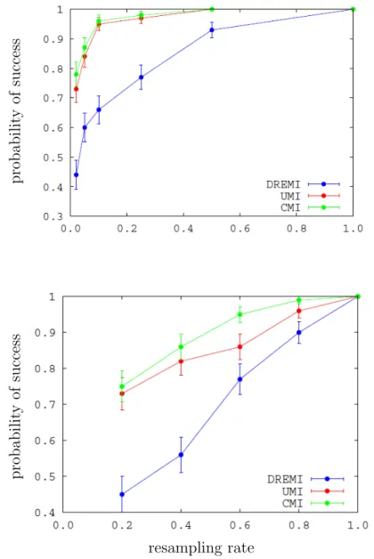
each time point in the same setting as [8] — and look to understand two distinct issues in our experiments with the flow-cytometry data. The first is whether the proposed quantities of UMI and CMI are able to capture the same biological trend that DREMI was able to capture. The second question relates to the sample complexity: How does the ability to recover the trend vary as a function of the sample complexity? To study this, we subsample the original data from [8] multiple times (100 in the experiments) at each subsam-pling ratio and compute the fraction of times we recover the true biological trend. This is plotted in Figure 5.1. The figure demonstrates that when the whole dataset is made available, UMI and CMI are able to spot the trend correctly (just as DREMI does). When fewer samples are available, UMI uniformly dominates DREMI and, in turn, CMI uniformly dominates UMI in terms of capturing the biological trend as a function of number of samples available. We believe that this strong empirical evidence lends credence to our approach. For completeness, we note that the datasets represented in

(24)

Figure 5.1 refer to regular T-cells (top figure) and T-cells exposed with an antigen (bottom figure), for which we expect different biological trends, but both of which are correctly captured by our metrics.

probabilit y of success probabilit y of success resampling rate

Figure 5.1: CMI and UMI estimators significantly improve over DREMI in capturing the biological trend in flow-cytometry data: the figures above refer to the same setting as Figure 6 of [8].

(25)

5.2 Synthetic Data

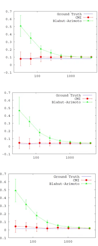
We demonstrate the accuracy of the proposed UMI and CMI estimators on synthetic experiments. We generate N samples from PXY where X is distributed as a beta distribution Beta(1.5,1.5) and Y = X + N, N ∼ N(0, σ2), independent of X. We present three results with varying σ2 ∈ {0.09,0.36,1.0}. Figure 5.2 shows the estimate of UMI, averaged over 100 instances. This is compared to the ground truth and the state-of-the-art partition-based estimators from [11]. The ground truth has been computed via simulations with 8192 samples from the desired distributionPY|XUX using Kraskov’s mutual information estimator [9].

For CMI, we use exactly the same distribution PXY as in UMI, but with varying σ2 _{∈ {0.36,}_1.0,_{2.25}, which is illustrated in Figure 5.3. Under the} power constraint, the ground truth is given by 1₂log(1 + σX2

σ2 N

) = 1₂log(1 + 1/16σ2). The proposed CMI estimator is compared agains the Blahut-Arimoto algorithm [30, 31] for computing discrete channel capacity, applied to quan-tized data. Both figures illustrate that the proposed estimators significantly improve over the state-of-the-art partition-based methods, in terms of sample complexity.

(26)

number of samplesN

Figure 5.2: The proposed UMI estimator significantly outperforms partition-based methods [11] in sample complexity. Additive Gaussian channels are used with varying variances σ2: 0.09 (top), 0.36 (middle), and 1.0 (bottom).

(27)

number of samples N

Figure 5.3: The proposed CMI estimator significantly outperforms

partition-based methods [30, 31] in sample complexity. Additive Gaussian channels are used with varying variances σ2: 0.36 (top), 1.0 (middle), and 2.25 (bottom).

(28)

CHAPTER 6 CONCLUSION AND DISCUSSION

In the thesis we have proposed novel information theoretic measures of po-tential influence of one variable on another, as well as provided novel estima-tors to compute the measures from i.i.d. samples. The technical innovation has been in proposing these estimators, by combining separate threads of methods in statistics (including importance sampling and nearest-neighbor methods). The consistency proofs suggest that a similar analysis the very popular estimator of (traditional) mutual information in [9] can be conduct-ed successfully; such work has been recently conductconduct-ed in [24]. Several other issues in statistical estimation theory intersect with our current work and we discuss some of these topics below.

• The main technical results of the thesis have been weak consistency of the proposed estimators. Proving stronger consistency guarantees and rates of convergence would be natural improvements, albeit chal-lenging ones. Rates of convergence in the nearest-neighbor methods are barely known in the literature even for traditional information the-oretic quantities: for instance, [26] derives a √N consistency for the single-dimensional case of differential entropy estimation (under strong assumptions on the underlying pdf), leaving higher-dimensional sce-narios open, and which recently have been successfully addressed in [24].

• There is a natural generalization of our estimators when the alphabet Y is high-dimensional, using thekNN approach (just as in the differen-tial entropy estimator of [10] or in the mutual information estimator of [9]). However, very recent works [20, 21, 32] have shown that boundary biases common in high-dimensional scenarios are much better handled using local parametric methods (as in [33, 34]). Adapting these ap-proaches to the estimators for UMI and CMI is an interesting direction

(29)

of future research.

• We have considered both the case of discrete and (single-dimensional) continuous alphabet X. The scenario of high-dimensional X is signif-icantly more challenging for CMI estimation: this is because of the (vastly) expanded space of distributions over which the optimization can be performed. Also challenging is to consider application-specific regularization of the inputs in this scenario.

• While the focus of the thesis has been on quantifying potential causal influence, a related question involves testing the direction of causality for a pair of random variables. This is a widely studied topic with a long lineage [4] but also of strong topical interest [7, 35, 6, 36]. A natural inclination is to explore the efficacy of UMI and CMI measures to test for direction of causality — especially in the context of the benchmark data sets collected in [6]. Our results are as follows: UMI has a 45% probability to predict the correct direction. CMI gives 53% probability. Directly comparing the marginal entropy H(X) andH(Y) by the esti-mator in [10] also only provides 45% accuracy. While in [6], different entropy estimators (with appropriate hyper parameter choices) were applied to get an accuracy up to 60%-70%. Further research is needed to shed conclusive light, although we point out that the benchmark datasets in [6] have substantial confounding factors that make causal direction hard to measure in the first place.

• The axiomatic derivation of potential causal influence naturally sug-gests CMI as an appropriate measure. We are also able to show that a more general quantity, the so-called R´enyi capacity, also meets the axioms. For any λ >0, λ6= 1, define R´enyi entropy:

Hλ(P) := 1

λ−1logEP[(dP) λ

] (6.1)

and R´enyi divergence: Dλ(PkQ) := 1 λ−1logEQ " dP dQ λ# . (6.2)

(30)

Now define the asymmetric information measure [37]: Kλ(PXPY|X) := inf

QY

Dλ(PXYkPXQY), (6.3)

which converges to the traditional mutual information when λ → 1. Now we can define the R´enyi capacity for any parameter λ and any fixed conditional distribution PY|X:

CMIλ := sup PX

inf QY

Dλ(PXYkPXQY). (6.4) Observe that asλ→1, we have CMIλ →CMI, the traditional Shannon capacity. We observe the following.

Proposition 2. For any λ >0, λ6= 1 we have that CMIλ satisfies the

axioms in Chapter 2.

The proof is available in Appendix C. In the light of this result, it would be interesting to design estimators for the more general family of R´enyi capacity measures and confirm their performance on empirical tasks such as the ones studied in [8]. It would also be very interesting to understand the role of additional axioms that would lead to the uniqueness of Shannon capacity (in the same spirit as entropy being uniquely characterized by somewhat similar axioms [3]).

• Another measure of information commonly used to quantify causal strength is directed mutual information (DMI): for a pair of random

vectors (X1, . . . , Xn) and (Y1, . . . , Yn) this quantity is defined as [38] n

X

k=1

I(X1, . . . , Xk;Yk|Y1, . . . , Yk−1). (6.5) While this quantity has been posited as a relevant metric in studying causality for a pair of sequences of observations (typically a time series) [39, 40], in the context of the thesis it simply reduces to the traditional mutual informationI(X;Y) (since we are studying only single random variables X and Y). If the random variables X and Y are vectors (sequences “in time”) and a causal structure is suspected “within” the components of X and Y, then CMI specializes to this setting readily

(31)

and could be used to quantify the causal influence, by computing the Shannon capacity of the time varying (Markov) channel from X and Y. In this context, CMI differs from DMI in the same sense as in the scalar random variable originally introduced in the thesis: CMI captures potential influence while DMI measures factual influence. • Finally, a comment on the optimization problem in CMI estimation:

the optimization problem involving the wi’s is not necessarily a con-cave program for a given sample realization, although this program converges to that of Shannon capacity computation (involving maxi-mizing mutual information), which is a concave function of the input probability distribution. Standard (stochastic) gradient decent is used in our experiments, and we did not face any disparity in convergent values over the set of synthetic experiments we conducted.

(32)

APPENDIX A

PROOF OF THEOREM 1

We present the proof of the theorem for two separate UMI estimators: first for continuousX and next for discreteX. We first state the formal assumptions under which the theorem holds.

Assumption 1. For continuous X, define

fU(y) ≡ Z

x

u(x)fY|X(y|x)dx, (A.1) fU(x

y) ≡ u(x)fY|X(y|x) fU(y)

. (A.2)

We make the following assumptions:

(a) R

fX,Y(x, y) logf(x, y) 2

dxdy <∞.

(b) There exists a finite constant C such that the Hessian matrix of H(f)

and H(fU) exists and max{kH(f)k2,kH(fU)k2} < C almost

every-where.

(c) There exists a positive constant C0 such that the conditional pdfs satisfy

fY|X(y

x)< C0 and fU(x

y)< C0 almost everywhere.

(d) There exist positive constants C1 < C2 such that the marginal pdf

sat-isfy, almost everywhere,

C1

µ(X) < fX(x)< C2 µ(X) .

(e) The bandwidth hN of the kernel density estimator is chosen as hN = 1

2N

−1/(2dx+3)_.

For discrete X, define

fu(y) ≡ X

x∈X

1

(33)

We make the following assumptions:

(a) R

fY|X(y|x) logfY|X(y|x) 2

dy <∞, for all x∈ X.

(b) There exists a finite constantCsuch that the Hessian matrix ofH(fY|X)

exists and kH(fY|X)k2 < C almost everywhere, for all x∈ X. (c) There exists a finite constantC0 such that the conditional pdffY|X(y

x)< C0 almost everywhere, for all x∈ X.

(d) There exists finite constants C1 < C2 such that the prior pX(x) > C1/|X | and fX(x)< C2/|X | almost everywhere.

A.1 The Continuous Alphabet Case

Given these assumptions, we define g(Xi, Yi) ≡ ψ(k) + log(N) + log

c_d

xcdy

cdx+dy

− log(nx,i) + log(ny,i)

, (A.4) such that ˆI_k,NU (X, Y) = _N1 PN_i=1 wig(Xi, Yi). Define each quantity with the true prior fX(x) as w0_i ≡ u(Xi) fX(Xi) , (A.5) n0_y,i ≡ X j6=i

w_j0_I{kYj −Yik< ρk,i}, (A.6) g0(Xi, Yi) ≡ ψ(k) + log(N) + log

c_d

xcdy

cdx+dy

− log(nx,i) + log(n0y,i)

, (A.7)

(34)

WithUX equal to the uniform distribution on the support ofX, we apply the triangle inequality to show that each term converges to zero in probability.

Iˆ_k,NU (X, Y)−IU(fY|X) = 1 N N X i=1 wig(Xi, Yi)− Z Z

u(x)fY|X(y|x) log

fY|X(y|x) R u(x0_)f Y|X(y|x0)dx0 dxdy ≤ 1 N N X i=1

wig(Xi, Yi)−w_i0g0(Xi, Yi) (A.8) + 1 N N X i=1 w_i0g0(Xi, Yi)− Z Z

u(x)fY|X(y|x) log

fY|X(y|x) R u(x0_)f Y|X(y|x0)dx0 dxdy , (A.9) The first term (A.8) captures the error in the kernel density estimator and we have the following claim, whose proof is delegated to Appendix A.1.1. Lemma 1. The term in Equation (A.8) converges to 0 as N → ∞ in prob-ability.

The second term in the error (A.9) comes from the sample noise in density estimation. Similar to the decomposition of mutual information, I(X;Y) = H(X) +H(Y)−H(X, Y), we decompose our estimator into three terms:

1 N N X i=1 w_i0g0(Xi, Yi) = Hb_k,NU (X) +Hb_k,NU (Y)−Hb_k,NU (X, Y) − N X i=1 w0_i

(35)

where b H_k,NU (X, Y) ≡ N X i=1 w0_i

N −ψ(k) +ψ(N) + logcdx+dy + (dx+dy) logρk,i

, (A.11) b H_k,NU (X) ≡ N X i=1 w0_i

N −lognx,i+ log(N −1) + logcdx+dxlogρk,i

, (A.12) b H_k,NU (Y) ≡ N X i=1 w0_i

N −logny,i+ log(N −1) + logcdy +dylogρk,i

. (A.13) Notice thatPN_i=1w0i

N(2 log(N −1)−ψ(N)−log(N)) goes to 0 as N goes to infinity. The desired claim follows directly from the following two lemmas showing the convergence each entropy estimates to corresponding entropies under UMI.

Lemma 2. Under the hypotheses of Theorem 1, for all ε >0 lim

N→∞P

Z Z

u(x)fY|X(y|x) log(fY|X(y|x)u(x))dxdy +Hb_k,NU (X, Y) > ε = 0 . (A.14) Lemma 3. Under the hypotheses of Theorem 1, for all ε >0

lim N→∞P

Z Z

u(x)fY|X(y|x) logfX(x) + logfU(y) dxdy +Hb_k,NU (X) +Hb_k,NU (Y) > ε = 0, (A.15)

where fU(y) = R fY|X(y|x)u(x)dx.

A crucial technical idea in proving these lemmas is the concept of impor-tance sampling. For any functionh(Xi, Yi), theimportance sampling estimate of _E[h] is given by ˜ hN = 1 N N X i=1 w0_ih(Xi, Yi), (A.16) where w_i0 = N u(Xi)/f(Xi). The following lemma gives the almost sure

(36)

convergence of ˜hn.

Lemma 4(Theorem 9.1 in [41]). Assume_E[h] =RR

u(x)fY|X(y|x)h(x, y)dxdy

exists, then P lim n→∞ ˜ hn=E[h] = 1.

A.1.1 Proof of Lemma 1

The term in Equation (A.8) is upper bounded by: 1 N N X i=1 wig(Xi, Yi)−wi0g 0 (Xi, Yi) ≤ 1 N N X i=1 wig(Xi, Yi)−wi0g 0 (Xi, Yi) ≤ 1 N N X i=1 |wi−wi0| |g 0 (Xi, Yi)|+wi g(Xi, Yi)−g0(Xi, Yi) = 1 N N X i=1

|wi−w_i0| |g0(Xi, Yi)|+wilog(ny,i)−log(n0_y,i) ≤ 1 N N X i=1

|wi−w_i0| |g0(Xi, Yi)|+winy,i−n0_y,i( 1 2ny,i + 1 2n0_y,i) ≤ 1 N N X i=1 |wi−w0i| |g 0_(X i, Yi)|+ N X i=1 wi N P_j₆_=i_I{kY_j −Y_i|< ρ_k,i}|w0_j−w_j| 2P j6=iI{kYj−Yi|< ρk,i}wj0 + P j6=iI{kYj −Yi|< ρk,i}|w 0 j−wj| 2P j6=iI{kYj−Yi|< ρk,i}wj ≤ 1 N N X i=1 |wi−w0i| |g 0 (Xi, Yi)|+ N X i=1 wi N max1≤j≤N|wj0 −wj| 2 min1≤j≤Nw0j +max1≤j≤N|w 0 j−wj| 2 min1≤j≤Nwj0 ≤ max 1≤i≤N|wi−w 0 i| max 1≤i≤N|g 0 (Xi, Yi)|+ 1 2 min1≤j≤Nw0j + 1 2 min1≤j≤N wj ), (A.17)

(37)

where the last inequality follows from the fact that PN_i=1wi =N. We upper bound each term as follows.

w_j0 = u(Xi) fX(Xi)

≥ 1/µ(K) C2/µ(K)

= 1/C2. (A.18)

Similarly we havew0_j ≤1/C1. This implies thatn0_y,i =P j6=iw

0

jI{kYi−Yjk ≤ ρk,i} ≥k/C2. For finite k and sufficiently largeN, we have:

g0(Xi, Yi) = ψ(k) + log(N) + log(cdxcdy cdx+dy )− log(nx,i) + log(ny,i) ≤ ψ(k) + log(N) + log(cdxcdy cdx+dy )− log(k) + log(k/C2) ≤ 2 logN , (A.19)

and similarly, using the fact thatny,i= P j6=iw 0 jI{kYi−Yjk ≤ρk,i} ≤N/C1, g0(Xi, Yi) ≥ ψ(k) + log(N) + log( cdxcdy cdx+dy )− log(N) + log(N/C1) ≥ −2 logN. (A.20)

We claim that for sufficiently largeN such that logN >max{C2ε/3,3C2/2}, if |wi−wi0|< ε/(3 logN) for all i, then (A.17) is upper bounded by ε.

max 1≤i≤N|wi−w 0 i| max 1≤i≤N|g 0 (Xi, Yi)|+ 1 2 min1≤j≤N wj0 + 1 2 min1≤j≤Nwj ) ≤ ε 3 logN 2 logN + C2 2 + 1 2/C2 − ε 3 logN ≤ ε 3 logN 2 logN + C2 2 +C2 ≤ε. (A.21)

Putting these bounds together, we have, for any ε >0 and sufficiently large N, P 1 N N X i=1 wig(Xi, Yi)−w0ig 0 (Xi, Yi) > ε ≤ _P max 1≤i≤N|wi−w 0 i|> ε 3 logN . (A.22)

(38)

Define

w_i00= _PNN/fX(Xi) j=1 1/fX(Xj)

, (A.23)

and applying the triangle inequality and union bound for (A.22), we have

For (A.24), recall thatw0_i =u(Xi)/fX(Xi). Sinceu(Xi)/fX(Xi)∈[1/C2,1/C1] for all i. Therefore,

P max 1≤i≤N|w 0 i−w 00 i|> ε 6 logN = _P max 1≤i≤N| u(Xi) fX(Xi) −_PNN/fX(Xi) j=1 1/fX(Xj) |> ε 6 logN = _P max 1≤i≤N u(Xi) fX(Xi) 1− N PN j=1 u(Xj)/fX(Xj) > ε 6 logN ≤ _P 1 C1 N X j=1 u(Xj) fX(Xj) −N> ε 6 logN N X j=1 u(Xj) fX(Xj) . ≤ _P N X j=1 u(Xj) fX(Xj) −N> ε 6 logN N C1 C2 . (A.26)

Note that w_j0 = u(Xj)

fX(Xj) are i.i.d. random variables with

E[w0j] = R fX(x)_fu(x) X(x)dx = 1 and w 0 j ∈ [1/C2,1/C1]. Therefore, by

(39)

Hoeffd-ing’s inequality, we obtain: P N X j=1 u(Xj) fX(Xj) −N> εN C1 6 logN C2 ≤ 2 exp ( − 2 εN C1 6 logN C2 2 N(1/C1−1/C2)2 ) = 2 exp − ε 2_{N C}4 1 18(logN)2_(C 2−C1)2 , (A.27)

which shows that the probability in (A.24) goes to 0 as N goes to infinity. For the probability in (A.25), recall that for any i,

|w_i00−wi| = N/fX(Xi) PN j=1 1/fX(Xj) − N/f˜X(Xi) PN j=1 1/f˜X(Xj) . (A.28) We use the following lemma that shows an upper bound for the error of the kernel density estimator.

˜ fX(Xi) = 1 (N −1)hdx N X j6=i K(Xj−Xi hN ). (A.29)

Lemma 5. Assume that K(u) ≤ A for all u, κj(K) = R

Rdx kuk

j_{K(u)du <} +∞ for any positive integer j ≥ 1 and R

RdxuK(u)du = 0. By choosing

hN = 1₂N−1/(2dx+3), we have for a given i∈ {1, . . . , N},

P fX˜ (Xi)−fX(Xi) > N−1/(2dx+3) ≤2 exp{−N 1/(2dx+3) 16A2 }. (A.30) Applying the union bound we can get that with probability at least 1− 2Nexp{−N1/(2dx+3)

16A2 }, we have

|f˜X(Xi)−fX(Xi)| < N−1/(2dx+3) (A.31) for all i. When this bound holds, we claim that the event inside of the probability in (A.25) holds for sufficiently large N. Together with (A.27), this proves the desired claim: for given ε >0 and large enough N,

1 N N X i=1 wig(Xi, Yi)−w0ig 0 (Xi, Yi) ≤ ε , (A.32)

(40)

with probability at least 1−2Nexp{−N1/(2dx+3) 16A2 } −2 exp{− ε2_{N C}4 1 18(logN)2_(C 2−C1)2}.

Now, we are left to show that (A.31) implies the event inside of the prob-ability in (A.25). Given (A.31), we have

|f˜X(Xi) fX(Xi) −1|< N −1/(2dx+3) fX(Xi) < µ(K)N −1/(2dx+3) C1 , (A.33)

for all i. Therefore, for sufficiently large N, wi−w0i is lower bounded by wi−w00i = N/fX(Xi) PN j=1 1/fX(Xj) − N/f˜X(Xi) PN j=1 1/f˜X(Xj) ≥ _PNN/fX(Xi) j=1 1/fX(Xj) 1− 1 + µ(K)N−_C1/(2dx+3) 1 1− µ(K)N−_C1/(2dx+3) 1 ≥ _PNN/fX(Xi) j=1 1/fX(Xj) 1−(1 + 3µ(K)N−1/(2dx+3) C1 ) (A.34) ≥ −3C2µ(K)N −1/(2dx+3) C2 1 , (A.35)

where (A.34) follows from the fact that (1 +a)/(1−a) ≤ 1 + 3a for a ∈ [0,1/3], and (A.35) follows from the fact thatC1/µ(K)≤fX(x)≤C2/µ(K). Similarly, it is upper bounded by

wi−w00i = N/fX(Xi) PN j=1 1/fX(Xj) − N/f˜X(Xi) PN j=1 1/f˜X(Xj) ≤ _PNN/fX(Xi) j=1 1/fX(Xj) 1− 1− µ(K)N−_C1/(2dx+3) 1 1 + µ(K)N−_C1/(2dx+3) 1 ≤ _PNN/fX(Xi) j=1 1/fX(Xj) 1−(1− 3µ(K)N−1/(2dx+3) C1 ) ≤ 3C2µ(K)N −1/(2dx+3) C2 1 . (A.36)

Here (A.36) comes from the fact that (1−a)/(1 +a)≥1−3a for all a ≥0. Therefore, |wi −w00i| ≤ 3C2µ(K)N−1/(2dx+3)/C12. For a given ε > 0 and for

(41)

Together with (A.22) and (A.27), this proves the desired convergence of the first term (A.8).

A.1.2 Proof of Lemma 5

Given Xi =x, denote aj = _h1dx N K(Xj−x hN ) such that ˜fX(Xi) = 1 N PN j=1aj. For sufficiently small hN, the mean of aj is given by:

E[aj] = Z z∈RdX 1 hdx N K(z−Xi hN )fX(z)dz = Z u∈RdX K(u)fX(x+hNu)du = Z u∈_RdX K(u) fX(x) +hNuT∇fX(x) +h2Nu T_H(f

X)(x)u+o(h2N))du = fX(x) +h2NC

Z

u∈_RdX

kuk2_K(u)du₊_o(h2

N), (A.38)

where we used the fact that the kernel is centered such thatR K(u)aT_udu₌ 0. For sufficiently small hN, we obtain |E[aj]−fX(x)|< hN. Therefore,

P f˜_X(X_i)−f_X(X_i) > N−1/(2dx+3) Xi =x ≤ _P N X j=1 aj −N fX(Xi) > N(2dx+2)/(2dx+3) Xi =x ≤ _P X j6=i aj −(N −1)E[aj] > N(2dx+2)/(2dx+3) −ai−N fX(x) + (N −1)E[aj] Xi =x . (A.39)

(42)

Since ai is bounded by A/hdNx, by choosing hN = 1₂N−

1

2dx+3, the right-hand

side is lower bounded by:

N(2dx+2)/(2dx+3)₋_a i −N fX(x) + (N −1)E[aj] ≥ N(2dx+2)/(2dx+3)_{− |a} i −fX(x)| −(N −1)|E[aj]−fX(x)| ≥ N(2dx+2)/(2dx+3)₋_A/hdx N −N hN ≥ 1 3N (2dx+2)/(2dx+3)_. _(A.40)

Since forj 6=i,a0_jsare i.i.d and bounded byA/hdx

N, by Hoeffding’s inequality, we obtain P X j6=i aj −(N −1)E[aj] > N(2dx+2)/(2dx+3) −ai−N fX(x) + (N −1)_E[aj] Xi =x ≤ _P X j6=i aj −(N −1)E[aj] > 1 3N (2dx+2)/(2dx+3) Xi =x ≤ 2 exp{−2( 1 3N (2dx+2)/(2dx+3)₎2 (N −1)·A2_h−2dx N } ≤ 2 exp{− 2 9A2_(N ₋₁₎(N (2dx+2)/(2dx+3)_hdx N) 2_} ≤ 2 exp{−N 1/(2dx+3) 9A2 }. (A.41)

Since this upper bound is independent of x, we can take expectation over x to obtain the desired claim.

A.1.3 Proof of Lemma 2

Define ˆ fX,Y(Xi, Yi) = exp{ψ(k)−ψ(N)} cdx+dyρ dx+dy k,i , (A.42) so that ˆ H_k,NU (X, Y) = − N X i=1 w0_i

(43)

By Theorem 8 of [42], we have lim

N→∞E

log ˆfX,Y(Xi, Yi)(Xi, Yi) = (x, y) = logfX,Y(x, y). (A.44) Notice that w_i0log ˆf(Xi, Yi) are identically distributed, therefore, by plugging in w_i0 =u(Xi)/fX(Xi), we have lim N→∞E ˆ H_k,NU (X, Y) = − lim N→∞E[w 0 ilog ˆfX,Y(Xi, Yi)] = − lim N→∞ Z Z E u(Xi) fX(Xi) log ˆfX,Y(Xi, Yi) (Xi, Yi) = (x, y) fX,Y(x, y)dxdy = − lim N→∞ Z Z u(x)fY|X(y|x)E log ˆfX,Y(Xi, Yi) (Xi, Yi) = (x, y) dxdy . (A.45) Now we want to show that

lim N→∞

Z Z

u(x)fY|X(y|x)Elog ˆfX,Y(Xi, Yi)(Xi, Yi) = (x, y)dxdy

= Z Z

u(x)fY|X(y|x) lim N→∞E log ˆfX,Y(Xi, Yi) (Xi, Yi) = (x, y) dxdy = Z Z

u(x)fY|X(y|x) logfX,Y(x, y)dxdy , (A.46) which follows from the reverse Fatou’s lemma and the fact that

lim sup N→∞ Z Z u(x) f(x)E log ˆfX,Y(Xi, Yi) (Xi, Yi) = (x, y) 2 f(x, y)dxdy ≤ C₁−2lim sup N→∞ Z Z E log ˆfX,Y(Xi, Yi) (Xi, Yi) = (x, y) 2 f(x, y)dxdy ≤ C₁−2 Z Z lim sup N→∞ E log ˆfX,Y(Xi, Yi) (Xi, Yi) = (x, y) 2 f(x, y)dxdy ≤ C₁−2 Z Z lim sup N→∞ logfX,Y(x, y) 2 f(x, y)dxdy < +∞. (A.47)

As explained in the main result section, we regularize the kNN distance such that ρdx+dy

k,i > Ck/N for some positive constant C. This ensures that log ˆfX,Y(Xi, Yi) < C0 almost surely. It follows that _E[log ˆfX,Y(Xi, Yi)|Xi = x, Yi = y] < C0 and one can apply reverse Fatou’s lemma. Similar

(44)

inter-change of limit has been used in [10, 16] without the regularization; in this context [17] claims that this step is not justified (although no counterexam-ple is pointed out). But in our case, given the practical way the algorithm is implemented with the regularization, reverse Fatou’s lemma is justified. Therefore, lim N→∞E ˆ H_k,NU (X, Y) = − Z Z

u(x)fY|X(y|x) logfX,Y(x, y)dxdy. (A.48) Moreover, by Theorem 11 of [42], we have:

lim

N→∞Var[ ˆfX,Y(Xi, Yi)] = (

Γ0(k) Γ(k))

0

Var[logfX,Y(x, y)], (A.49) and for any j 6=i:

lim

N→∞Cov[ ˆfX,Y(Xi, Yi),

ˆ

fX,Y(Xj, Yj)] = 0 . (A.50) Byw_i0 ≤1/C1 for all iand the fact that ˆfX,Y(Xi, Yi) are identically distribut-ed, we have: VarHˆ_k,NU (X, Y) = N X i=1 (w_i0)2 N2 Var[ ˆfX,Y(Xi, Yi)] + X j6=i w_i0w0_j

N2 Cov[ ˆfX,Y(Xi, Yi),fˆX,Y(Xj, Yj)] ≤ N X i=1 1 C2 1N2 Var[ ˆfX,Y(Xi, Yi)] + X j6=i 1 C2 1N2

Cov[ ˆfX,Y(Xi, Yi),fˆX,Y(Xj, Yj)]

= 1 C2 1N ((Γ 0_(k) Γ(k)) 0

Var[logfX,Y(x, y)])

+ 1 C2 1N2 N 2

Cov[ ˆfX,Y(X1, Y1),fX,Yˆ (X2, Y2)]. (A.51) Therefore,

lim N→∞Var

_ˆ

(45)

Combining (A.48) and (A.52), we get: lim N→∞E h b H_k,NU (X, Y)− − Z Z

u(x)fY|X(y|x) logfX,Y(x, y)dxdy 2i = lim N→∞ EHˆk,NU (X, Y)− − Z Z

u(x)fY|X(y|x) logfX,Y(x, y)dxdy 2 + lim N→∞Var _ˆ H_k,NU (X, Y) = 0. (A.53) Therefore, ˆHU

k,N(X, Y) converges to its mean inL2, and hence in probability, i.e., lim N→∞P bH_k,NU (X, Y) + Z Z

u(x)fY|X(y|x) logfX,Y(x, y)dxdy > ε

= 0.

(A.54)

A.1.4 Proof of Lemma 3

Define ˆ fX(Xi) ≡ nx,i (N −1)cdxρ dx k,i , (A.55) ˆ fU(Yi) ≡ ny,i (N −1)cdyρ dy k,i , (A.56) such that ˆ H_k,NU (X) + ˆH_k,NU (Y) = − N X i=1 w_i0 N log ˆfX(Xi) + log ˆfU(Yi) . (A.57)

(46)

By triangle inequality, we can write the formula in Lemma 3 as:

Z Z

u(x)fY|X(y|x) logfX(x) + logfU(y) dxdy+Hb_k,NU (X) +Hb_k,NU (Y) = Z Z

u(x)fY|X(y|x) logfX(x) + logfU(y) dxdy − N X i=1 w_i0 N log ˆfX(Xi) + log ˆfU(Yi) ≤ Z Z

u(x)fY|X(y|x) logfX(x) + logfU(y) dxdy − N X i=1 w_i0 N logfX(Xi) + logfU(Yi) (A.58) + N X i=1 w0_i N log ˆfX(Xi) + log ˆfU(Yi) − logfX(Xi) + logfU(Yi) .(A.59) The first term (A.58) comes from sampling. Recall thatw0_i =u(Xi)/fX(Xi). Since the random variables w0_i logfX(Xi) + logfU(Yi)

are i.i.d., therefore, by the strong law of large numbers,

N X

i=1 w0_i

N logfX(Xi) + logfU(Yi)

→_E u(x) fX(x)

logfX(x) + logfU(y)

, (A.60) almost surely. The mean is given by

E

u(x) fX(x)

(logfX(x) + logfU(y))

= Z Z

u(x) fX(x)

logfX(x) + logfU(y)

f(x, y)dxdy =

Z Z

u(x)fY|X(y|x) logfX(x) + logfU(y)

dxdy. (A.61) Therefore, (A.58) converges to 0 almost surely.

The second term (A.59) comes from density estimation. To simplfy the notations, let Zi = (Xi, Yi), z = (x, y) and f(z) = f(x, y). For any fixed

(47)

ε >0, by union bound, we obtain that P N X i=1 w0_i N

(log ˆfX(Xi) + log ˆfU(Yi))−(logfX(Xi) + logfU(Yi)) > ε ≤ _P N [ i=1

(log ˆfX(Xi) + log ˆfU(Yi))−(logfX(Xi) + logfU(Yi)) > ε/2 +_P( N X i=1 w0_i >2N). (A.62)

The second term converges to zero by Lemma 4. The first term is bounded by: P N [ i=1

(log ˆfX(Xi) + log ˆfU(Yi))−(logfX(Xi) + logfU(Yi)) > ε/2 ≤ N ·_P (log ˆfX(Xi) + log ˆfU(Yi))−(logfX(Xi) + logfU(Yi))

> ε/2

≤ N Z

(I1(z) +I2(z) +I3(z) +I4(z) )f(z)dz (A.63) where I1(z) = P ρk,i> r1 Zi =z , (A.64) I2(z) = P ρk,i< r2 Zi =z , (A.65) I3(z) = Z r1 r=r2 P log ˆf_X(X_i)−logf_X(X_i) > ε/4 ρ_k,i =r, Z_i =z fρk,i(r)dr , (A.66) I4(z) = Z r1 r=r2 P log ˆf_U(Y_i)−logf_U(Y_i) > ε/4 ρk,i =r, Zi =z fρk,i(r)dr , (A.67)

where fρk,i(r) is the pdf of ρk,i givenZi =z. Here

r1 = logN(N f(z)cdx+dy) − 1 dx+dy _(A.68) r2 = max(logN)2(N fX(x)cdx) −1 dx_,_(log_N₎2_{(N fU}_(y)cd y) −1 dy _}._(A.69)

I1(z) and I2(z) are the probability that the k-NN distance ρk,i is large or small given Zi =z. I3(z) and I4(z) gives the probability that the estimator deviates from the true value, given thatρk,iis medium. We will consider the

(48)

four terms separately.

I1: Let BZ(z, r) = {Z : kZ −zk < r} be the (dx +dy)-dimensional ball centered at z with radius r. Since the Hessian matrix of H(f) exists and kH(f)k2 < C almost everywhere, then for sufficiently smallr, the probability mass within BZ(z, r) is given by

P u∈BZ(z, r)= Z ku−zk≤r f(u)du = Z ku−zk≤r f(z) + (u−z)T∇f(z) + (u−z)TH(f)(z)(u−z)du ∈ f(z)cdx+dyr dx+dy₍₁₋_Cr2_{)), f(z)c} dx+dyr dx+dy_{(1 +}_Cr2₎₎_. _(A.70)

Then for sufficiently large N, the probability mass withinBZ(z, r1) is lower bounded by p1 ≡ P u∈BZ(z, r1) ≥ f(z)cdx+dyr dx+dy 1 1−Cr 2 1 ≥ (logN) dx+dy 2N . (A.71)

I1(z) is the probability that at mostksamples fall in BZ(z, r1), so it is upper bounded by I1(z) = P ρk,i> r1 Zi =z = k−1 X m=0 N −1 m pm₁ (1−p1)N−1−m ≤ k−1 X m=0 Nm(1−p1)N−1−m ≤ kNk−1(1−(logN) dx+dy 2N ) N−k−1 ≤ kNk−1exp{−(logN) dx+dy_(N ₋_k₋₁₎ 2N } ≤ kNk−1exp{−(logN) dx+dy 4 }, (A.72) for any dx, dy ≥1.

(49)

I2: Letr2,1 ≡(logN)2(N fX(x)cdx)

− 1

dx. Then for sufficiently large N, the

probability mass within BZ(z, r2,1) is given by: p2,1 ≡ P u∈BZ(z, r2,1) ≤ f(z)cdx+dyr dx+dy 2,1 1 +Cr 2 2,1 ≤ 2f(z)cdx+dy (f(x)cdx) dx+dy dx (logN)2(dx+dy)_N−dx+dy_dx ≤ 2fY|X(y|x) cdx+dy cdx (logN)2(dx+dy)_N−dx+dy_dx ≤ 2C0cdx+dy cdx

(logN)2(dx+dy)_N−dx+dy_dx _, _(A.73)

where the last equation comes from the assumption that fY|X(y|x) < C0. Similarly, let r2,2 = (logN)2(N fU(y)cdy)

− 1

dy_{, the probability of being in}

BZ(z, r2,2) is p2,2 ≡ _P u∈BZ(z, r2,2) ≤ f(z)cdx+dyr dx+dy 2,2 1 +Cr2,22 ≤ 2f(z)cdx+dy (fU(y)cdy) dx+dy dy (logN)2(dx+dy)_N− dx+dy dy ≤ 2 f(z) fU(y) cdx+dy cdy (logN)2(dx+dy)_N− dx+dy dy ≤ 2C2 fU(x, y) fU(y) cdx+dy cdy (logN)2(dx+dy)_N− dx+dy dy ≤ 2C2C0 cdx+dy cdy (logN)2(dx+dy)_N− dx+dy dy _. _(A.74)

(50)

It is upper bounded as follows:

I2(z) = _P ρk,i<maxr2,1, r2,2}Zi =z = N−1 X m=k N −1 m max{p2,1, p2,2}m(1− {p2,1, p2,2})N−1−m ≤ N−1 X m=k Nmmax{p2,1, p2,2}m ≤ N−1 X m=k ( 2C0C2 cdx+dy min{cdx, cdy} (logN)2(dx+dy)_N−min{ dy dx, dx dy}m ≤ (4C0C2 cdx+dy min{cdx, cdy} )k(logN)2k(dx+dy)_N−kmin{ dy dx, dx dy} _, _(A.75)

for sufficiently largeN such that_minc_{dx+dy_c

dx,cdy}(logN) 2(dx+dy)_N−min{ dx+dy dx , dx+dy dy } _<

1/(4C0), the last inequality comes from sum of geometric series. This holds for any dx, dy ≥1 andk ≥1.

I3: Given that Zi = z = (x, y) and ρk,i = r. Recall that ˆfX(Xi) = nx,i (N−1)cdxρdxk,i , so we have P log ˆf_X(X_i)−logf_X(X_i) > ε/4 ρk,i =r, Zi =z

= _P logn_x,i−log(N −1)c_d_xrdxf_X(x) > ε/4 ρk,i =r, Zi =z = _P nx,i >(N −1)cdxr dx_fX_(x)eε/4_ρk,i₌_{r, Zi} ₌_z +_P nx,i <(N −1)cdxr dx_f X(x)e−ε/4 ρk,i =r, Zi =z . (A.76) Given Zi =z and ρk,i=r∈[r2,1, r1], the probability distribution ofnx,i is given in the following lemma.

Lemma 6. Given Zi = z = (x, y) and ρk,i = r < rN for some

determin-istic sequence of rN such that limN→∞rN = 0 and for any positive ε > 0,

the number of neighbors nx,i −k is distributed as PN_l=k+1−1 Ul, where Ul are i.i.d Bernoulli random variables with mean fX(x)cdxr

dx₍₁−_ε/8) ≤

E[Ul] ≤ fX(x)cdxr

(51)

Given Lemma. 6, we obtain P nx,i >(N −1)cdxr dx_fX_(x)eε/4 ρk,i=r, Zi =z = _P N−1 X l=k+1 Ul >(N −1)cdxr dx_fX_(x)eε/4₋_k = _P N−1 X l=k+1 Ul−N0E[Ul]>(N −1)cdxr dx_f X(x)eε/4−k−N0E[Ul] , (A.77) where N0 =N−k−1 for simplicity. Here the right-hand side in the proba-bility is lower bounded by

(N −1)cdxr dx_f X(x)eε/4−k−E[Ul] ≥ (N −1)cdxr dx_f X(x)eε/4−k−N0fX(x)cdxr dx_{(1 +}_ε/8) ≥ N0cdxr dx_f X(x)(eε/4−1−ε/8)−k ≥ N0cdxr dx_f X(x)ε/16, (A.78)

for sufficiently large N such that N0cdxr

dx_f

X(x)(eε/4−1−ε/16)> k. Since Ul is Bernoulli, we have E[Ul2] = E[Ul]. Now applying Bernstein’s inequali-ty, (A.77) is upper bounded by:

P N−1 X l=k+1 Ul−N0_E[Ul]>(N −1)cdxr dx_fX_(x)eε₋_k₋_N0 E[Ul] ≤ _P N−1 X l=k+1 Ul−N0E[Ul]> N0cdxr dx_f X(x)ε/16 ≤ exp{− (N 0_c dxr dx_f X(x)ε/16)2 2 N0 E[Ul2] + 1 3(N 0_cd xrdxfX(x)ε/16) } ≤ exp{− (N 0_cd xr dx_fX_(x)ε/16)2 2 N0_c dxrdxfX(x)(1 +ε/8) + 1 3(N 0_c dxrdxfX(x)ε/16) } = exp{− ε 2 512(1 + 7ε/48)N 0 cdxr dx_fX_(x)}_. _(A.79)

(52)

Similarly, the tail bound on the other direction is given by: P nx,i <(N −1)cdxr dx_fX_(x)e−ε/4 ρk,i =r, Zi =z = _P N−1 X l=k+1 Ul<(N −1)cdxr dx_fX_(x)e−ε/4₋_k = _P N−1 X l=k+1 Ul−N0E[Ul]<(N −1)cdxr dx_f X(x)e−ε/4−k−N0E[Ul] , (A.80) where the right-hand side is negative and upper bounded by:

(N −1)cdxr dx_f X(x)e−ε/4−k−E[Ul] ≤ (N −1)cdxr dx_f X(x)e−ε/4−k−(N−k−1)fX(x)cdxr dx₍₁₋_ε/8) ≤ N0cdxr dx_f X(x)(e−ε/4−1 +ε/8) ≤ −N0cdxr dx_f X(x)ε/16, (A.81)

for small enough r such that cdxr

dx_f

X(x)e−ε/4 ≤ 1 and small enoughε that e−ε/4₋_{1 + 3ε/16}_<_{0. Similarly, (A.80) is upper bounded by:}

P N−1 X l=k+1 Ul−N0E[Ul]<(N −1)cdxr dx_f X(x)e−ε/4−k−N0E[Ul] ≤ exp{− ε 2 512(1 + 7ε/48)N 0 cdxr dx_f X(x)}. (A.82)

Therefore,I3(z) is upper bounded by: I3(z) = Z r1 r=r2 P log ˆfX(Xi)−logfX(Xi) > ε ρk,i=r, Zi =z fρk,i(r)dr ≤ Z r1 r=r2,1 P log ˆf_X(X_i)−logf_X(X_i) > ε ρk,i=r, Zi =z fρk,i(r)dr ≤ Z r1 r=r2,1 2 exp{− ε 2 512(1 + 7ε/48)N 0 cdxr dx_f X(x)}fρk,i(r)dr ≤ 2 exp{− ε 2 1024N cdxfX(x)((logN) 2_{(N f} X(x)cdx) − 1 dx)dx} ≤ 2 exp{− ε 2 1024(logN) 2dx_}_, _(A.83)

(53)

for sufficiently large N such thatN0/(1 + 7

48ε)> N/2.

I4: Given that Zi = z = (x, y) and ρk,i = r. Recall that ˆfU(Yi) = ny,i (N−1)cdyrdy, then we have P log ˆf_U(Y_i)−logf_U(Y_i) > ε/4 ρk,i=r, Zi =z

= _P logn_y,i−log(N −1)c_d_yrdyf_Y(y) > ε/4 ρk,i=r, Zi =z = _P ny,i >(N −1)cdyr dy_fU_(y)eε/4_ρk,i ₌_{r, Zi} ₌_z +_P ny,i<(N −1)cdyr dy_f U(y)e−ε/4 ρk,i=r, Zi =z . (A.84) Recall that ny,i= X j6=i w_j0_I{kYj −Yik< ρk,i}= X j6=i u(Xi) fX(Xi)I

{kYj −Yik< ρk,i}. (A.85)

We write ny,i=m (1) y,i +m (2) y,i, where m(1)_y,i = X j:kZj−zk<ρk,i u(Xj) fX(Xj) m(2)_y,i = X j:kZj−zk>ρk,i u(Xj) fX(Xj)I

{kYj−Yik< ρk,i}. (A.86)

SinceC1/µ(K)≤fX(Xj)≤C2/µ(K), we have: k/C2 ≤m (1)

y,i ≤k/C1. Given that Zi = z and ρk,i = r ∈ [r2,2, r1], the probability distribution of m

(2) y,i is given by the following lemma.

Lemma 7. Given Zi = z = (x, y) and ρk,i = r < rN for some deter-ministic sequence of rN such that limN→∞rN = 0 and for a positive ε > 0,

the distribution of m(2)_y,i is distributed as PN_l=k+1−1 Vl where Vl are i.i.d

ran-dom variables with Vl ∈ [0,1/C1] and mean fU(y)cdyr

dy₍₁₋_ε/8)_≤

E[Vl] ≤ fU(y)cdyr

Conditional dependence via Shannon capacity: axioms, estimators and applications

ABSTRACT

ACKNOWLEDGMENTS

TABLE OF CONTENTS

CHAPTER 1

INTRODUCTION

CHAPTER 2

AN AXIOMATIC APPROACH

2.1

Axioms on Influence Measures

2.2

Real-Valued Alphabets

CHAPTER 3

ESTIMATORS

3.1

Uniform Mutual Information

3.2

Capacitated Mutual Information

CHAPTER 4

CONVERGENCE GUARANTEES

4.1

Uniform Mutual Information

4.2

Capacitated Mutual Information

CHAPTER 5

NUMERICAL EXPERIMENTS

5.1

Gene Causal Strength from Single Cell Data

5.2

Synthetic Data

CHAPTER 6

CONCLUSION AND DISCUSSION

APPENDIX A

PROOF OF THEOREM 1

A.1

The Continuous Alphabet Case

A.1.1

Proof of Lemma 1

A.1.2

Proof of Lemma 5

A.1.3

Proof of Lemma 2

A.1.4

Proof of Lemma 3